Full Terms & Conditions of access and use can be found at
http://www.tandfonline.com/action/journalInformation?journalCode=ubes20
Download by: [Universitas Maritim Raja Ali Haji] Date: 11 January 2016, At: 19:35
Journal of Business & Economic Statistics
ISSN: 0735-0015 (Print) 1537-2707 (Online) Journal homepage: http://www.tandfonline.com/loi/ubes20
Frequentist Evaluation of Small DSGE Models
Gunnar Bårdsen & Luca Fanelli
To cite this article: Gunnar Bårdsen & Luca Fanelli (2015) Frequentist Evaluation of Small DSGE Models, Journal of Business & Economic Statistics, 33:3, 307-322, DOI: 10.1080/07350015.2014.948724
To link to this article: http://dx.doi.org/10.1080/07350015.2014.948724
View supplementary material
Accepted author version posted online: 08 Aug 2014.
Submit your article to this journal
Article views: 311
View related articles
View Crossmark data
Supplementary materials for this article are available online. Please go tohttp://tandfonline.com/r/JBES
Frequentist Evaluation of Small DSGE Models
Gunnar B ˚
ARDSENDepartment of Economics, Norwegian University of Science and Technology, Dragvoll 7491, Trondheim, Norway ([email protected])
Luca FANELLI
Department of Statistical Sciences and School of Economics, Management and Statistics, University of Bologna
I-40126, Bologna, Italy ([email protected])
This article proposes a new evaluation approach for the class of small-scale “hybrid” new Keynesian dynamic stochastic general equilibrium (NK-DSGE) models typically used in monetary policy and business cycle analysis. The empirical assessment of the NK-DSGE model is based on a conditional sequence of likelihood-based tests conducted in a vector autoregressive (VAR) system, in which both the low- and high-frequency implications of the model are addressed in a coherent framework. If the low-high-frequency behavior of the original time series of the model can be approximated by nonstationary processes, stationarity must be imposed by removing the stochastic trends. This gives rise to a set of recoverable unit roots/cointegration restrictions, in addition to the short-run cross-equation restrictions. The procedure is based on the sequence “LR1→LR2→LR3,” where LR1 is the cointegration rank test, LR2 is the cointegration matrix test, and LR3 is the cross-equation restrictions test: LR2 is computed conditional on LR1 and LR3 is computed conditional on LR2. The Type I errors of the three tests are set consistently with a prefixed overall nominal significance level. A bootstrap analog of the testing strategy is proposed in small samples. We show that the information stemming from the individual tests can be used constructively to uncover which features of the data are not captured by the theoretical model and thus to rectify, when possible, the specification. We investigate the empirical size properties of the proposed testing strategy by a Monte Carlo experiment and show the empirical usefulness of our approach by estimating and testing a monetary business cycle NK-DSGE model using U.S. quarterly data. Supplementary materials for this article are available online.
KEY WORDS: LR test; Maximum likelihood; New-Keynesian model; VAR.
1. INTRODUCTION
Dynamic stochastic general equilibrium (DSGE) models are dominating macroeconomics, in academic research, as well as in economic policy making. Even though these models, by their very nature, cannot provide a complete description of the busi-ness cycle and of any time series, such as inflation, output, and the policy rate, they are widely used to evaluate macroeconomic scenarios and predict economic activity. Assessing the corre-spondence between what these models imply and what the data tell us is therefore a crucial step in the process of analyzing policy options and their effects, especially if one takes the view that the scientific validity of a model should not be exclusively based on its logical coherence or its intellectual appeal, but also on its ability to make empirical predictions that are not rejected by the data; see, for example, De Grauwe (2010) and Pesaran and Smith (2011).
There are several methods that can used to evaluate the em-pirical performance of DSGE models, depending on the specific objectives of the analysis. Most common methods include eco-nomic reliability, statistical fit, and forecasting accuracy; see, for example, Schorfheide (2000), An and Schorfheide (2007), and Schorfheide (2011). Each evaluation method is based on a “metric” and different “metrics” may lead to different con-clusions. Our “metric” will be based on testing the restrictions on the data implied by DSGE models. This approach is by no means new, but dates back to the early literature on the econometrics of rational expectations models; see Hansen and Sargent (1980,1981), Wallis (1980), and Johansen and Swensen (1999).
It is often claimed that Bayesian techniques are preferable to standard likelihood-based methods because DSGE models typically represent a false description of the data-generating process (DGP) and misspecification can be important in estima-tion; see, for example, Canova and Ferroni (2012). Schorfheide (2000) suggested using a loss function to assess the discrepancy between DSGE model predictions and overall posterior distribu-tion of the populadistribu-tion characteristics that the researcher is trying to match. Del Negro et al. (2007) developed a set of tools within the Bayesian approach that can be used for assessing the time se-ries fit of a DSGE model based on a systematic relaxation of the set of cross-equation restrictions (CER) that the structural model implies on the vector autoregressive (VAR) representation of the data. Their method, known as the “DSGE-VAR” approach, pro-vides the investigator with a Bayesian “metric” through which he/she can evaluate how far/close the DSGE model is from a VAR approximation of the data.
While misspecification in DSGE models is a concrete possi-bility, we do not think it represents a strong argument against the idea of confronting these models with data by frequentist (classical) methods. The knowledge that the DSGE model is “misspecified” in some directions may help the investigator un-derstand what features of the data the model is missing, how important these features are, and, possibly, how to improve the original specification.
© 2015American Statistical Association
Journal of Business & Economic Statistics
July 2015, Vol. 33, No. 3 DOI:10.1080/07350015.2014.948724
307
We propose a frequentist evaluation approach for a class of small-scale DSGE models grounded in the new Keynesian tra-dition and relevant for economic policy analysis, henceforth denoted with the acronym “NK-DSGE” models. These models were investigated by among many others, Clarida, Gal´ı, and Gertler (2000), Lubik and Schorfheide (2004), Ireland (2004), Christiano, Eichenbaum, and Evans (2005), Smets and Wouters (2007), DeJong and Dave (2011), Carlstrom, Fuerst, and Paus-tian (2009), Benati and Surico (2009), and more generally, in Woodford (2003) and Gal´ı (2008). They feature both macroe-conomic and monetary policy shocks and typically include a forward-looking aggregate demand equation, a Phillips curve, and a monetary policy reaction function. They can also ac-commodate the monetary/fiscal policy mix (e.g., Bianchi2012) and/or financial frictions, for example, Castelnuovo and Nistic`o (2010).
In principle, there are two types of restrictions that can be tested in NK-DSGE models. First, there are the long-run cointegration/common-trend restrictions stemming from the ob-servation that there are generally more variables to be modeled than there are independent integrated forcing processes; see, for example, Canova, Finn, and Pagan (1994), S¨oderlind and Vredin (1996), Fukaˇc and Pagan (2010), and Juselius (2011). Importantly, these restrictions hold regardless of the unique-ness/multiplicity of the model solution and are invariant to the specification of the transient dynamics of the system—see Broze, Gourieroux, and Szafarz (1990) and Binder and Pesaran (1995). Second, there are the short-run CER that apply to the system conditional on the common trends. The long-run and short-run properties of NK-DSGE models are generally inter-dependent and therefore they should be examined jointly. Our method is based on testing both types of restrictions in a coher-ent framework. We propose a sequcoher-ential procedure computed in three steps using likelihood ratio (LR) tests. We first test whether the cointegration rank (the number of stochastic common trends) is consistent with the predictions of the NK-DSGE model, us-ing a finite-order VAR model. Next, we test the implied over-identifying cointegrating restrictions, conditional on the chosen rank. Finally, we test the CER the NK-DSGE model places on the VAR system, conditional on the cointegrating restrictions. Overall, the suggested method involves computing a sequence of LR tests, called LR1 (LR cointegration rank test), LR2 (LR cointegration matrix test), and LR3 (LR test for CER). The test LR2 is run conditional upon LR1 not rejecting the cointegration rank, and LR3 is run if LR2 does not reject the over-identifying cointegration restrictions. To our knowledge, King et al. (1991), Canova, Finn, and Pagan (1994), and S¨oderlind and Vredin (1996) are early examples of the use of the test LR1 in related contexts. Juselius (2011) is a recent example of the use of the test LR2 in the NK-DSGE models, while Guerron-Quintana, In-oue, and Kilian (2013) proposed the inversion of a test like LR3 to build confidence sets for structural parameters that are robust to identification failure. For ease of exposition, we denote our testing strategy with the symbol ‘‘LR1→LR2→LR3.” The novelty of the “LR1→LR2→LR3” procedure is that the em-pirical evaluation of the NK-DSGE model is treated as a multiple hypothesis testing approach. This is one of the contributions of our approach, as we will show in the rest of the article.
Under the null of the NK-DSGE model, the tests LR1, LR2, and LR3, individually considered, are correctly sized in the sense that their asymptotic size is equal to the prefixed nominal Type I error. Accordingly, using simple Bonferroni arguments, we can prove that the overall asymptotic size of the testing strategy does not exceed the sum of the Type I errors prefixed for each test. If a practitioner wishes to test the NK-DSGE model at, say, the 5% nominal level of significance, the critical values of the tests LR1, LR2, and LR3 can be chosen such that the sum of the individual Type I errors does not exceed 5%. The size of the overall testing strategy can be kept under strict control in small samples by referring to the bootstrap analog of the “LR1→
LR2→LR3” procedure. In this case, the bootstrap version of the test LR1 is computed following Cavaliere, Rahbek, and Taylor (2012). The bootstrap counterpart of the test LR2 is computed as in Boswijk et al. (2013) and Cavaliere, Nielsen, and Rahbek (2014)—see Gredenhoff and Jacobson (2001) for an alternative approach. The bootstrap analog of the test LR3 can be computed as in, for example, Cho and Moreno (2006) or Fanelli and Palomba (2011).
A discrepancy is often found between what the data tell and what theory implies when long-run restrictions are tested in structural forward-looking models. For instance, the balanced-growth-path property of the standard neoclassical growth model implies that hours worked are stationary. This, however, appears to be at odds with the persistent movements of per capita hours in the data. Similarly, NK-DSGE models typically maintain that inflation is a stationary process. In small samples, however, we typically observe high inflation persistence. The possible fail-ures of the common-trend/cointegration restrictions using the tests LR1 and LR2 are generally the hardest features to inter-pret because of the lack of indications about how to modify the model. Chang, Doh, and Schorfheide (2007) illustrated how the specification of a real business cycle DSGE model can be modi-fied to incorporate nonstationary labor supply shocks that gener-ate permanent shifts in hours worked. Similarly, Juselius (2011) provided a detailed interpretation of monetary business cycle NK-DSGE models, under different scenarios reflecting the com-mon trends that might be found in the data. As we show below, proper modifications to the probabilistic structure of the exoge-nous shocks that generate fluctuations in NK-DSGE models can be used to generalize trend structures and close the gap between theory and data. Likewise, when the short-run CER implied by the NK-DSGE model are rejected by the LR3 test, one should think of alternative structural frameworks to capture the dynamic features of the data, or the omitted transmission mechanisms of the shocks. For example, dynamically rich, distributed-lag small-scale monetary models have been employed by, Estrella and Fuhrer (2002, 2003) and Fuhrer and Rudebusch (2004), among others, while medium-scale systems that involve a rela-tively larger number of variables were considered by Christiano, Eichenbaum, and Evans (2005) and Smets and Wouters (2007). Thus, we go beyond using the “LR1→LR2→LR3” testing strategy as an “accept–reject” proposition. We show that the outcomes of the individual tests can be used constructively to uncover what features of the data are not captured by the theo-retical model and to rectify, when possible, the specification of the NK-DSGE model.
We evaluate the empirical performance of the “LR1→
LR2→LR3” testing strategy by a small Monte Carlo experi-ment whose DGP belongs to the monetary business cycle NK-DSGE model discussed in Benati and Surico (2009), which is the leading example used in our article. We further show the empirical usefulness of our approach by estimating and testing the NK-DSGE model of Benati and Surico (2009) using U.S. quarterly data.
Our article has several connections with the existing litera-ture. Canova, Finn, and Pagan (1994) and S¨oderlind and Vredin (1996) proposed a method to evaluate real business cycle models by eliciting the (highly) restricted VAR representation underly-ing them and comparunderly-ing it with an unrestricted VAR for the data. They recognize that the driving forces in these models may be integrated, and hence account for the implied set of cointegra-tion restriccointegra-tions, as well as considering what Canova, Finn, and Pagan (1994) call the “noncointegrating restrictions.” Our ap-proach differs from Canova, Finn, and Pagan (1994) and S¨oder-lind and Vredin (1996) in the way the “LR1→LR2→LR3” testing strategy is designed. Fukaˇc and Pagan (2010) proposed an evaluation approach to NK-DSGE models in which both the long and short-run behavior of the data are taken into ac-count by modeling the common stochastic trends in an error-correction framework. While Fukaˇc and Pagan (2010) put forth a “limited information” approach, our analysis is developed in a “full information” maximum likelihood (ML) framework. Also, Juselius (2011) applied a “full information” ML approach, but he limits his attention to the steady-state implications of NK-DSGE models, leaving the CER untested. Gorodnichenko and Ng (2010) proposed robust estimators for the parameters of DSGE models that do not require researchers to take a stand on whether the shocks have permanent or transitory effects, while “filtering” is implicitly obtained in our framework by a proper transformation of the model through the cointegration restrictions. The approach of Gorodnichenko and Ng (2010) is therefore suitable when the exact underlying cointegrating relationships are not known. Moreover, Gorodnichenko and Ng (2010) were not concerned with assessing how far/close is the estimated model from/to the data. One advantage of our method is that if the NK-DSGE model is not rejected by the data, it automatically delivers the ML estimates of the struc-tural parameters, while the extension of Gorodnichenko and Ng’s (2010) method to the case of ML estimation is not always practical.
Finally, apart from the Bayesian approach, we have many points in common with the “DSGE-VAR” approach of Del Ne-gro et al. (2007). These authors also used a cointegrated VAR in error-correction form as the statistical model for the data, but they impose the common-trend restrictions without testing. The prior distribution for the VAR parameters in Del Negro et al. (2007) is centered on the CER implied by the DSGE model and has dispersion governed by a scalar (hyper)parameter, denoted λ, such that small values ofλindicate that the VAR is far from the theoretical model, while large values ofλindicate that the theoretical model is supported by the data. A cutoff value forλ is not provided, as noticed by Christiano (2007). In our testing strategy, the test LR3 plays a role similar toλin Del Negro et al. (2007). However, we have by construction a cutoff value for LR3, which depends on prefixed nominal Type I error: values
of LR3 smaller than the cutoff value indicate that the VAR is “close” to the NK-DSGE model, and vice versa.
The article is organized as follows. We introduce the base-line NK-DSGE model and its assumptions in Section 2 and discuss a set of testable restrictions, which are usually ignored in the literature, in Section3. We present our testing strategy in Section4and investigate its empirical size performance by a simulation experiment in Section5. We present an empirical il-lustration in which our reference NK-DSGE model is evaluated on U.S. quarterly data in Section6. Section7concludes the ar-ticle. The Appendix discusses the asymptotic size of the testing strategy. Additional details about the ML estimation algorithm for the structural parameters necessary to compute the test LR3, as well as detailed interpretation of the estimates obtained in the simulation experiment and in the empirical illustration, are reported in a technical supplement.
2. MODEL AND ASSUMPTIONS
Our starting point is the structural representation of a typical NK-DSGE model that aims at capturing the stylized features of the business cycle. The model is in the form of a system resulting from the log-linearization around steady-state values of the equations that describe the behavior of economic agents. LetWtbe thep-dimensional vector collecting all the variables
of interest. A typical structural monetary NK-DSGE model takes the form of the linearized rational expectations model:
AW0 Wt=AWfEtWt+1+AWb Wt−1+ηWt , (1)
where AW
0 ,A
W f, andA
W
b are p×pmatrices whose elements
depend on the structural parameters collected in the vectorθ, andηW
t is a mean zero vector of structural disturbances. The term
EtWt+1=E(Wt |Ft) denotes conditional expectations, where Ftis the available stochastic information set at timetand is such thatσ(Wt, Wt−1,. . . , W1)⊆Ft, whereσ(Wt, Wt−1,. . . , W1) is
the sigma field generated by the variables. As is standard in the literature, we posit that the structural disturbance termηW
t obeys
a vector autoregressive processes of order one, that is,
ηWt =RWηtW−1+u
W t , u
W
t ∼WN(0p×1, W,u), (2)
where RW is a diagonal stable matrix (i.e., with eigenvalues
lying inside the unit disk) anduWt is a white-noise term with co-variance matrixW,u. Hereafter,uWt will be denoted the vector
of structural or “fundamental” shocks, and it will be assumed that dim(uW
t )=dim(Wt)=p, preventing the occurrence of the
“stochastic singularity” issue; see, for example, Ireland (2004) and DeJong and Dave (2011). In general, theory does not provide information about the correlation of the structural disturbances across equations; if cross-equation correlations are assumed for the structural disturbances, these can be captured by specify-ing a nondiagonal covariance matrix W,u. In our setup, the
nonzero elements ofRWand of vech(W,u) belong to the vector
of structural parametersθ. All meaningful values ofθ belong to the “theoretically admissible” (compact) parameter space, denotedP.
A solution of model (1)–(2) is any stochastic process
Wt∗∞t=0, Wt∗ =Wt∗(θ), such that, for θ ∈P, EtWt∗+1=
E(W∗
t+1|Ft) exists and if Wt∗ is substituted for Wt into the
structural equations, the model is verified for eacht, for fixed
initial conditions. A reduced form solution is a member of the solution set whose time series representation is such that Wt
depends onuW
t , lags ofWt anduWt (and, possibly, other
arbi-trary martingale difference sequences (MDS) with respect toFt
independent ofuW
t , called “sunspot shocks”).
We confine the class of reduced-form solutions associated with the NK-DSGE model to a known family of linear models by the assumption that follows.
Assumption 1 (Determinacy). The “true” valueθ0ofθ is an
interior point ofP∗, whereP∗⊂Pis such that, for eachθ ∈P∗,
the NK-DSGE model (1)–(2) has a unique and asymptotically stationary (stable) reduced-form solution.
Assumption 1 can be interpreted as the null hypothesis that the DGP belongs to the unique stable solution of the NK-DSGE system (1)–(2). This assumption is standard in the literature and hinges on the idea that the time series upon which model (1) is built and estimated are typically constructed (or conceptualized) as stationary deviations from steady-state values.
Under Assumption 1, the unique stable solution of the model (1)–(2) can be represented as the asymptotically stationary VAR system
trices that depend nonlinearly onθ through the implicit set of nonlinear CER: and ˜W,ε is the covariance matrix ofεWt under the constraints,
see Binder and Pesaran (1995), Uhlig (1999), Kapetanios, Pa-gan, and Scott (2007), and Fanelli (2012).
In general, the NK-DSGE model represented in Equations (1)–(2) reads as a “partial equilibrium” model, in the sense that it does not specify how any unobservable components of Wt, denotedWtu, are generated. For instance, in the examples
we discuss below, the NK-DSGE model specified in the form (1)–(2) is based on the output gap and takes as given the process generating the natural level of output.
Let Wo
t be the subvector of Wt that contains the
observ-able variobserv-ables. Given the n-dimensional “complete” vector Zt=(Wto′, W
u
t)′, n≥p, which collects, without any loss of
generality, the observed (first) and unobserved variables (last), one can interpret the (stationary) vectorWt in systems (1) and
(3) as obtained from the linear combination
Wt=ζ′Zt, (7)
where ζ is a knownn×p matrix of full column-rankp that combines the observed and unobserved variables and/or picks out the stationary elements ofZtthat enter the structural model.
A further step toward the “complete” specification of the NK-DSGE model is provided by Assumption 2.
Assumption 2 (Unobserved processes are integrated of
or-der one).The subvector Wu
t is such that Wtu is covariance
stationary.
Assumption 2 simply states thatWtu is integrated of order one, denotedWtu∼I(1). It does not provide a detailed specifi-cation of the process generating the unobserved variables, but it can be further specialized according to the specific features of the model under investigation, as shown in the next sub-sections. Given the scope of the present article, approximating the unobserved components withI(1) processes meets two re-quirements. First, Assumption 2 formalizes the property that the NK-DSGE model features stochastic trends. Second, theI(1) assumption may represent a reasonable and interpretable choice for the typical unobservable components that characterize the class of small-scale NK-DSGE models used in monetary policy and business cycle analysis, that is, the natural level of output (potential output) and/or the inflation target (or trend inflation), as suggested by Bekaert, Cho, and Moreno (2010), Fukaˇc and Pagan (2010), and Section2.1.
Given Assumptions 1 and 2 and a detailed specification of the process generating Wtu, the “complete” (fully specified) NK-DSGE model can be given the structural representation
AZ0Zt =AZfEtZt+1+AZbZt−1+ηZt (8)
where the matricesAZ
0,A
Z f,A
Z
b, andu,Znot only depend on
θ, but also on a set of additional parameters, denoted withθa,
which are associated with the processes specified forWu t. The
“extended” vector of structural parameters is therefore given byθe=(θ′, θa′)′. Compared to the formulation (1)–(2) of the
NK-DSGE model, the system represented in Equations (8) and (9) incorporates the unit-root implication of Assumption 2. We will refer to the representation in Equations (8) and (9) as the “complete” specification of the NK-DSGE model. It is worth remarking that, albeitWt in Equation (7) reads as a subvector
of Zt, Wt has the representation in Equations (3)–(6) under
Assumption 1.
The next subsection provides a detailed example about the relationship between the representation in Equations (1) and (2) and (8) and (9) of the NK-DSGE model.
2.1 An Example Model
We use an example based on Benati and Surico (2009). The model consists of the following equations:
˜
hence Wt=( ˜yt, πt, it)′, p=3, ηWt =(ηy,t˜ , ηπ,t, ηi,t)′, and
t is the natural rate
of output;πt is the inflation rate andit is the nominal interest
rate;ηy,t˜ ,ηπ,t, andηi,tare stochastic disturbances autocorrelated
of order one, whileuy,t˜ ,uπ,t, andui,t can be interpreted as
de-mand, supply, and monetary shocks, respectively. The structural parameters are collected in the vectorθ=(γ,δ,̺,κ,κ, ρ,ϕπ,
ϕy,ρy˜,ρπ,ρi,σy2˜, σπ2, σ
2
i)
′ and their economic interpretation
may be found in Benati and Surico (2009).
The model (1)–(2) is “incomplete” according to our defini-tion, because it does not specify the process for the natural level of outputytp. One way to “complete” the model is to specialize
Assumption 2 as follows:
Assumption 3 (Potential output is a random walk).
ytp =y p
t−1+ηyp,t , ηyp,t ∼WN(0, σy2p). (14)
In addition to the nonstationarity hypothesis, Assumption 3 pro-vides a simple DGP forytp consistent with the representation
in Equations (8) and (9), see below. The usual interpretation of Assumption 3 is that the flexible price level of outputytp
is driven by a combination of a stationary demand shock and a nonstationary technology shock, as in Ireland (2004). In this framework, the vectorWt =( ˜yt, πt, it)′ can be thought of as
being obtained through the linear combination in Equation (7), which here qualifies in the expression
Wt=
Given the relationship in Equation (15), the Equations (10)–(13) jointly with Equation (14) imply the following configuration of the matricesA0,Af, andAb:
The relationships between Wt andZt defined by Equation
(7) and the representation in Equations (8) and (9) of the NK-DSGE model can conveniently be used to analyze the whole set of testable restrictions. Under Assumptions 1 and 2,Zt ∼I(1),
and all cointegration/common-trend restrictions of the system are subsumed in the vector Zt. The model that captures the
CER after factoring out the cointegrating relations from the system is given by the finite-order VAR representation forWtin
Equations (3)–(6). In this section, we explore the set of testable implications related to the vectorZt, while in the next section we
exploit these implications to define a coherent testing strategy for the NK-DSGE model.
We consider the n-dimensional vector of transformed vari-ables
where β0 is the n×r identified cointegration matrix,β0⊥ is
its orthogonal complement, and τ is a (n−r)×r selection matrix that is restricted so that it is not orthogonal to β0⊥.
The role of τ is to pick out a proper set of variables in first differences from the vector (1−L)Zt = Zt, whereLis the
lag operator (LjZt=Zt−j). The choice ofτ in Equation (16)
is not necessarily unique, however. The case discussed below shows that, despite the many possible choices ofτ, not all of them are consistent with the theoretical features of the NK-DSGE model. In principle,β0may temporarily depend on some
“additional” parameters that we collect in the vector ν, and which are not necessarily related toθ. We writeβ0=β0(ν) to
make clear such a dependence. Under the null hypothesis that the NK-DSGE model is valid, and with all constraints implied by the NK-DSGE model imposed on the system forZt, the joint
restriction
r=p, β0=β0b =ζ (17)
must hold, where the symbolβ0bdenotes the counterpart of the identified cointegration matrix β0 that leads to what we shall
define below as a “balanced” (error-correction) representation of the NK-DSGE model. Equation (17) maintains that, under the null of the NK-DSGE model, the identified cointegration matrixβ0b must be equal to the selection matrixζ of Equation (7) and, accordingly, must not depend on any parameter. Hence, the dependence ofβ0 onνis suppressed in Equation (17). We
observe that the transformation in Equation (16) mimics the one used by Campbell and Shiller (1987) to address the analysis of present value models through VAR systems.
Under the restriction (17), we can recover Wt from Yt as
nonsingular by construction, the mapping in Equation (16) can be used in the model in Equation (8) to obtain
AZ0G(β0, τ,1−L)−1Yt =AZfG(β0, τ,1−L)−1EtYt+1
+AZbG(β0, τ,1−L)−1Yt−1+ηZt .
(18)
The appealing feature of the representation in Equation (18) is that, other than involving stationary variables (i.e., those in Yt), the (inverse of the) difference operator (1−L) cancels
out from the equations if one restrictsβ0as in Equation (17),
and imposes a proper set of restrictions on θ, such that the transformed model is “balanced.” With the term “balanced,” we mean thatG(β0, τ,1−L)−1is replaced withG(β0b, τ,1−L)−1
and some restrictions are placed on the elements ofθ, so all left-hand and right-left-hand side variables appearing in system (17) are stationary. The nature of these restrictions will be demonstrated in the examples that follow.
Hereafter we use the representation
AY0Yt =AYfEtYt+1+AYbYt−1+ηYt (19)
ηtY =RYηYt−1+u
Y
t (20)
to denote the “balanced” counterpart of system (18). The sys-tems (19) and (20) can be regarded as an error-correction rep-resentation of the NK-DSGE model.
The structural parameters in the matricesAY0,AYf,AYb,RY,
are collected in the vector θY, where
θY is obtained fromθe by imposing the restrictions that map
system (18) into the transformed representation in Equations (19) and (20). In general, dim(θY)=dim(θe)−c, wherecis
the total number of restrictions onθenecessary for balancing.
Under Assumptions 1 and 2 (and the other minor assumptions in Section 2), if the unique stable solution of the NK-DSGE model (19)–(20) exists, it can be represented in the form
Yt =˜1Yt−1+˜2Yt−2+εYt , ε
onθY through the set of nonlinear CER:
t under the constraints, see Section2. The
con-straints in Equations (22)–(24) mimic those derived in Equa-tions (4)–(6) for the “original” specification of the NK-DSGE model, but here refer to the “complete” specification based on Assumption 2.
We now come back to our leading example, analyzed in Section2.1, to discuss some situations that clarify the essence of the transformations fromZttoYtand the resulting set of testable
restrictions. In particular, Section3.1deals with the “desirable” situation in which the number of common stochastic trends
found in the data,n−r, lines up with the number predicted by the theory,n−p, and the identified cointegration relationships match perfectly the structure in Equation (17). Section 3.2
deals, instead, with the situation where the inferred number of common trends,n−r, is larger thann−p(r < p), hence the structure of the cointegration relationships in Equation (17) is no longer valid. We argue that, in these cases, it is generally possible to rectify the specification of the structural equations to feature the “additional” stochastic trends, provided these trends can be given a sensible economic interpretation. This process, however, may give rise to extra (testable) restrictions in other parts of the model. Finally, Section3.3deals with the case in which it is necessary to think about alternative specifications of the transmission mechanisms of the shocks. This situation may arise when the CER in Equations (22)–(24) (or in Equations (4)–(6) if the “incomplete” specification is investigated) are not valid.
3.1 Example 1: The Case of a Single Stochastic Trend
Consider the NK-DSGE model in Equations (10)–(13) and Assumption 3. Suppose that givenZt =(yt, πt, it, y
p
t )′, the
se-lected cointegration rankrand the identified cointegration rela-tionshipsβ0perfectly match the requirements in Equation (17),
that is, In this case, the output gap, inflation, and the short-term inter-est rate are jointly stationary and there is a single stochastic trend inZt. The cointegration relationships in Equation (25) are
consistent with the hypothesis that the system is driven by a non-stationary technology shock; see, for example, Ireland (2004) and DeJong and Dave (2011).
Equation (18) generates the system
˜
where we have left the operator (1−L)−1in the final equation
to highlight the point about balancing. To see that (1−L)−1
cancels out from the former equation, it is sufficient to rewrite
it in the form (using Assumption 3)
˜
yt =y˜t−1+ yt+ηy∗p,t, (27)
where ηy∗p,t = −ηyp,t. It is worth emphasizing that Equation (27) is a reparameterization of the random walk model assumed forytpin Equation (14). A similar representation obtains if the chosenτ inG(βb
well as the vectorηYt in the representation in Equation (19), can easily be derived and are equal to
AY0 = strictions relative to the strictly observable time series in Zt,
Zto=(yt, πt, it)′=Wto∼I(1), are
whererois the cointegration rank associated withZo t .
3.2 Example 2: The Case of Two Stochastic Trends
Consider the NK-DSGE model in Equations (10)–(14). Imag-ine that, givenZt =(yt, πt, it, y
p
t)′, the selected cointegration
rank isr =2=p, implying the existence ofn−r=4−2=2 stochastic trends, one more than the technology trend predicted by the baseline version of the model. We discuss in detail two possible scenarios that can be used to nest a setup like this, denoted Scenario 1 and Scenario 2, respectively.
Scenario 1: stochastic inflation target. Inflation is typically a highly persistent process, which can sometimes be approx-imated reasonably well by I(1) processes. If the quantity
̺
1+̺κ + κ
1+̺κ in the NKPC in Equation (11) is close to 1, the
I(1) approximation forπt is sensible in small samples. While
it is implicitly assumed that trend inflation is zero in the system (10)–(13), it may be the case that trend inflation is determined by the long-run target of the central bank’s policy rule. A drift in trend inflation could therefore be attributed to shifts in that target. Consider, for instance, the small monetary NK-DSGE model investigated by Bekaert, Cho, and Moreno (2010). Their model differs from our leading example only in the specification of the policy rule, which in their framework is given by
it =ρit−1+(1−ρ)ϕπ(Etπt+1−πt∗)+(1−ρ)ϕyy˜t+ηi,t,
(29)
whereπ∗
t is a stochastic inflation target generated by the
equa-tion
policy stance regarding the long-term rate of inflation, assumed to be iid, and the parameter̟measures the extent to which the monetary authority smoothes the inflation target in anchoring its inflation target to a properly defined measure of the “long-run inflation expectations,”πLR=(1−̺)∞j=0̺jEtπt+j (see eq.
(9) in Bekaert, Cho, and Moreno2010). Therefore, with̟ =0, the targetπ∗
t equals long-run inflation expectations in the
ab-sence of exogenous shifts, while, for values of̟ close or equal to unity, Equation (30) collapses to the random walk model: π∗
t =πt∗−1+ǫπ∗,t.If this model can be taken as a reasonable
description of the evolution of π∗
t in the sample, πt andπt∗
must be cointegrated with cointegration vector (1,−1) for the monetary policy rule in Equation (29) to be balanced (note that, ifπt−πt∗is stationary, (Etπt+1−πt∗) also will be stationary).
Under this DGP, the investigator will find two stochastic trends inZt =(yt, πt, it, y
p
t)′and the source of the cointegration rank
failure (i.e.,r < p) will be the omitted stochastic inflation tar-get. A necessary condition for this hypothesis to be valid is that it holds the restriction
The specification in Equation (31) implies thatypt andπt are
I(1) andyt−y p
t anditare stationary. The testable cointegration
restrictions relative to the strictly observable time seriesZo t =
(yt, πt, it)′=Wtocollapse to
ro=1 , (0,0,1,0)Zto∼stationary. (32)
Scenario 2: stationary real (ex-post) interest rate. Suppose
that the two cointegration relationships identified from the data are given by
whereνis a cointegration parameter not related to the structural parametersθe. The two cointegrating vectors in Equation (33) are the output gap and a linear combination ofit andπt with
cointegration vector (1, −ν). For values of the parameter ν close to one, the stationary linear combination (it−νπt) can be
interpreted as a measure of the ex-post real interest rate. Hence, other than the technology trend, we can think about a real interest rate trend (or Fisher parity relationship). The mapping fromZt
toYtis in this case given by
and by imposing this transformation on the system (10)–(13), the analog of the system (18) is given by
To make only the stationary variables in Yt enter the model,
we need to eliminate the operator (1−L)−1from the equations
above. This is achieved by imposing the following additional restrictions:ν=ϕπ =κ=1, which, after some algebraic
ma-nipulations, lead to the equations
˜
This new system is the counterpart of the error-correction rep-resentation of the NK-DSGE system (19)–(20). It is balanced because it does not involve variables other than those in Yt.
The vector of structural parameters isθY =(γ,δ,̺,ρ,ϕy,ρy˜,
is the number of restrictions required for balancing. The inter-pretation of the transformed system is not trivial. The policy rule in Equation (36) is now expressed such that the “opera-tional/implementation target” is the real interest rate, while the decision variables are the output gap and the change in inflation
(the so-called “acceleration rate”). The conditionϕπ =1
main-tains that the long-run response of the Central Bank to inflation is equal to one, which stands in sharp contrasts with a widely shared view about the conquest of the U.S. inflation during the “Great Moderation” era; see, for example, Clarida, Gal´ı, and Gertler (2000) and Lubik and Schorfheide (2004). The restric-tionκ=1 implies “full indexation” and the Phillips curve in
Equation (35) is expressed as a “purely forward-looking” model for πt.In this case, the testable cointegration restrictions
rela-tive to the strictly observable time seriesZot =(yt, πt, it)′=Wto
correspond to
ro=1, (0,−ν,1,0)Zto∼stationary, withν=1. (38)
One can compare the two scenarios by testing whether, for r=2 (ro=1), the cointegration relationship is better described
by the structure in Equation (31) (Equation (32)), or the structure in Equation (33) (Equation (38)), using the testing strategy we introduce in the next section.
3.3 Example 3: The Cost Channel
Consider again the leading example model in Equations (10)– (14) but suppose now that the short-run CER implied by this system, summarized in Equations (4)–(6) (Equations (22)–(23)), are not valid for the sample period used to evaluate the model. One might conjecture, for instance, that this occurs because the baseline specification does not account for a cost-channel that might be at work in the economy. In short, a share of firms in the economy might need to borrow resources to pay workers’ wages before the final goods market opens. According to this theory, see Christiano, Eichenbaum, and Evans (2005) and Ravenna and Walsh (2006), the policy rate also should enter firms’ marginal costs as a proxy of the interest rate paid on their loans, leading to the system
In this model, the parameter 0≤κi<1 captures the share of
firms acceding the financial markets. The implied set of CER obtained with 0< κi <1 are different in the absence of a cost
channel based onκi=0.
4. THE TEST SEQUENCE
We consider the NK-DSGE model introduced in Section2, Assumptions 1 and 2, and focus on the following hypotheses
H0: the DGP belongs to system (21)–(24) ;
H1: the DGP does not belong to system (21)–(24). (39)
The null in Equation (39) will also be referred to as the null that “the NK-DSGE model is valid.”H0implicitly maintains that the
cointegration/common-trend restrictions subsumed in Equation (17) are fulfilled, hence it is possible to mapZt intoYt. Thus,
any testing strategy forH0againstH1is a conditional decision
rule.
To simplify the exposition without altering the logic of our method, we assume temporarily that all variables in Zt (and
hence inYt) can be observed. We turn to the role of
unobserv-ables later. Consider the VAR model forZt:
Zt = ℓ
j=1
PjZt−j +μdt+ξt , ξt ∼WN(0n×1, ξ), (40)
wherePj,j =1, . . . , ℓaren×nmatrices of parameters,ℓis
the lag order,dt is a vector including deterministic variables
(constant, linear trend dummies, etc.) with associated matrix of coefficients, μ, andξt is a white-noise disturbance. Consider
also the corresponding error-correction representation
Zt =αβ′Zt−1+
ℓ−1
j=1
j Zt−1+μdt+ξt ,
ξt ∼WN(0n×1, ξ), (41)
whereαβ′=(ℓ
j=1Pj −In),αis the n×r matrix of
adjust-ment coefficients, β is the n×r cointegration matrix, and j = −ℓh=j+1Ph, j =1, . . . , ℓ−1. Suppose that the VAR
lag order,ℓ, is determined from the data and that the vector of deterministic components,dt, is selected in accordance with
the time series features observed for the variables inZt. Our
procedure is based on the following steps:
LR1 [Cointegration rank test]. We estimate the VAR
sys-tem (40) and test for the hypothesis that the cointegration rank isr =p, corresponding ton−pcommon stochastic trends driving the system, against the alternative r=n, corresponding to a stationary system. We suggest using ei-ther the “one-shot” version of the LR Trace test (Johansen
1996), henceforth denoted LR1, or its “sequential” ver-sion, denoted LR1seq. The LR1seqtest involves starting with
r=0 (nstochastic trends), testing in turn the hypothesis “the cointegration rank isr” against “the VAR is station-ary” forr=0, . . . , n−1, until, for a given value ofr=r,ˆ the asymptoticp-value associated with the test statistics ex-ceeds the chosen significance level. The bootstrap versions of these tests discussed by Cavaliere, Rahbek, and Taylor (2012) can be applied in small samples. If the hypothesis r=pis not rejected, we consider the next step. If instead the hypothesisr=pis rejected, we suggest proceeding by thinking about an alternative specification that embodies, when possible, the stochastic trends not featured by the original specification of the NK-DSGE model; see as an example the cases discussed in Section3.2.
LR2 [Over-identification cointegration restrictions test].
Givenr=p, we move to the vector error-correction coun-terpart of the cointegrated VAR in Equation (41), and fix the (identified) cointegration matrixβat the structure implied by the theoretical model, that is,β=β0b=ζas in Equation (17). Then we compute an LR test, henceforth denoted with LR2, for the implied set of over-identifying restrictions; see Johansen (1996). The bootstrap versions of the test LR2 discussed in, for example, Boswijk et al. (2013) and Cava-liere, Nielsen, and Rahbek (2014) can be used to improve the small sample performance. If the LR2 test does not reject the over-identifying restrictions, we build the
trans-formed vectorYtin Equation (16) by keepingβ =β0b =ζ
fixed at the nonrejected structure, and consider the next step. If instead the LR2 test rejects the restrictions, one can proceed similarly to the case in which the LR1 (LR1seq)
test rejects the predicted number of stochastic trends.
LR3 [Test for CER]. We estimate the finite-order VAR system
in Equation (21) unrestrictedly, that is, leaving the matrices 1,2, andY,εunconstrained, and imposing the CER in
Equations (22)–(24), using the ML algorithm summarized in the technical supplement. We thus compute an LR test for the CER, henceforth denoted LR3, and obtain the ML estimate of the structural parameters. The LR3 test can also be constructed by referring to the “partial equilibrium” representation of the NK-DSGE model for Wt, given by
the system in Equations (3)–(6). When computationally feasible, bootstrap versions of the test LR3 discussed in, for example, Cho and Moreno (2006) and adapted from Fanelli and Palomba (2011) can be used in small samples.
The “LR1→LR2→LR3” testing strategy is a novel ap-proach in the literature. From a statistical viewpoint, H0 in
Equation (39 ) is rejected in favor ofH1 if one of the three
tests rejects, while it is accepted if all three tests pass. However, the “LR1→LR2→LR3” testing strategy need not be applied mechanically as an “accept–reject” proposition. The informa-tion, stemming from the tests LR1 (LR1seq), LR2, and LR3,
can potentially be used to uncover which features of the data or transmission mechanisms of the shocks are not captured by the theoretical model, so that the model may be improved; see, for example, the scenarios discussed in Sections3.2and3.3. In principle, it is possible to follow the alternative strategy based on imposing (without testing) the restrictions in Equation (17) on the VAR, testing the CER alone. While such a strategy is advantageous when the restrictions imposed are “true,” one of its perils is that insisting that a root very close to unity is a stationary root, for example, may lead to large size distortions and power losses in tests for the CER in rational expectations models; see Johansen (2006) and Li (2007).
The “LR1→LR2→LR3” testing strategy discussed so far maintains that the econometrician observes all components of Zt (and hence of Yt). When it is not possible to proxy
all variables, the testing strategy can be adapted. In these cases, the testable cointegration/common-trend implications of the NK-DSGE model reflect on the subvector Zo
t =Wto of
Zt. For instance, considering the examples discussed in
Sec-tions3.1and3.2, the relevant log run testable restrictions are given in Equations (28), (32), and (38), respectively. In this case, Wo
t has a state-space (VARMA-type) representation
un-der the null H0 in Equation (39) (see the technical
supple-ment), and a finite-order VAR forWtocan provide, with qualifi-cations, a reasonable approximation of its actual time series properties. The procedure is based on the following testing steps:
LR1 [Cointegration rank test: the case of unobservables].
We specify a VAR forWo
t similar to system (40) with a
relatively “large”ℓ, and use the test(s) LR1 and/or LR1seq
to select the cointegration rankro.
LR2 [Over-identification cointegration restrictions test:
the case of unobservables]. We use the vector
error-correction counterpart of the cointegrated VAR sim-ilar to system (41) and, fixing ro, we compute the
LR2 test by considering the over-identifying cointegration restrictions.
LR3 [Test for CER: the case of unobservables]. We
com-pute the LR3 test by evaluating the likelihood function associated with the “minimal state-space representation” associated with the system (21) under the CER in Equa-tions (22)–(24) (or the system (3) under the CER in Equa-tions (4)–(6)) with the Kalman filter; see, for example, Ruge-Murcia (2007) and Fukaˇc and Pagan (2010). We re-fer to Komunjer and Ng (2011) and Guerron-Quintana, Inoue, and Kilian (2013) for practical examples where the “minimal state-space representation” is derived from the set of observationally equivalent nonminimal state-space representations. An alternative to the test LR3 based on the indirect inference approach may be found in the technical supplement.
Under the nullH0in Equation (39), the asymptotic properties
of each of the three tests comprising the “LR1→LR2→LR3” testing strategy are known. The asymptotic properties of the tests LR1 (LR1seq) and LR2 may be found in Johansen (1996), while
the asymptotic properties of their bootstrap counterparts were discussed by Cavaliere, Rahbek, and Taylor (2012), Boswijk et al. (2013), and Cavaliere, Nielsen, and Rahbek (2014)—see also Gredenhoff and Jacobson (2001). The asymptotic proper-ties of the test LR3 are standard (including its bootstrap ana-log) under standard regularity conditions. We have postponed a detailed derivation of the asymptotic size properties of the “LR1→LR2→LR3” testing strategy to the Appendix. Be-cause the three tests are asymptotically correctly sized under the null, if the test forH0 againstH1 in Equation (39) is
con-ducted by fixing the overall significance level at, for example, the 5% level, the Type I errors (and hence the critical values) of the tests LR1 (LR1seq), LR2, and LR3 must be chosen
accord-ingly, for example, 1% for LR1 (LR1seq), 2% for LR2, and 2%
for LR3.
It is worth spending a few words on the tests LR1 and LR1seq.
In our framework, the use of the “one-shot” cointegration rank test LR1 reflects the idea that the number of common trends driving the variables are given and equal to n−r0=n−p
under the null of the NK-DSGE model, where r0 is the true
cointegration rank. By construction, the LR1 test rules out all alternatives in which the number of common trends is, for exam-ple, larger thann−p, and in which its asymptotic distribution is unknown, if, for instance,r0< p. The LR1 test must be
ap-plied, therefore, when one is confident that there are no more thann−pstochastic trends in the data. Instead, the LR1seqtest
has power asymptotically against the alternative of a number of stochastic trends different fromn−p. Nevertheless, its finite sample performance may be poor, as our simulation experi-ment in the next section will docuexperi-ment, and therefore it should be applied and interpreted with caution. When the empirical evaluation of the NK-DSGE model is based on theWto=Zto subvector, it is also possible to apply a number of alternative tests to LR1 and LR1seq. These are reviewed in, for example,
L¨utkepohl and Claessen (1997); see also Stock and Watson (1988).
5. SIMULATION EXPERIMENT
To evaluate the finite sample size performance of the ‘‘LR1→LR2→LR3” testing strategy, we conduct a small Monte Carlo experiment based on the determinate solution of the model summarized in Equations (10)–(14). We fix the dis-count rate̺at the value̺=0.99, and consider the estimation of ωf =̺/(1+̺κ) and derive that of κ indirectly. Hence,
the vector of free structural parameters is given byθ=(γ,δ, ωf,ρ,ϕπ,ϕy,ρy˜,ρπ,ρi,σy2˜, σπ2, σ
2
i)
′and the “extended”
vec-tor isθe=(θ′,θa)′, whereθa=σy2p(ηyp,t =uyp,t). The vector of fundamental shocksuZ
t =
uy,t˜ , uπ,t, ui,t, uyp,t
′
is assumed white noise with Gaussian distribution and diagonal covariance matrixu,Z. The parameter vectorθis calibrated to the
empiri-cal estimates of Benati and Surico (2009); see, in particular, the last column of theirTable 1(“after the Volcker stabilization”). The variance of the natural rate of outputσ2
ypis fixed at a value considered reasonable. Recall that, in this setup,θY =θe. The
calibrated values ofθe are reported in the first column of Ta-ble 1, panel 2. In line with the developments in the empirical illustration of Section6, we assume that the econometrician can observe the natural rate of output,ytp.
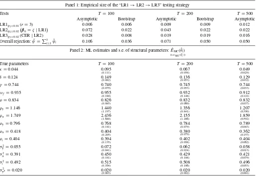
We generate time series of sizeT = 100, 200, and 500, and compute the test sequence “LR1→LR2→LR3”M=5000 times. The overall nominal level of significance is fixed at 5% (ψ=0.05), and the nominal Type I errors of the three tests are 1% for the LR1 test (ψ1=0.01), 2% for the test LR2 (ψ2=
0.02), and 2% for the test LR3 (ψ3=0.02). The (asymptotic)
critical values are chosen accordingly.
The results are summarized inTable 1, panel 1. For samples of sizeT =100 and 200, we also compute the (iid) bootstrap ver-sions of the tests. The implementation of the bootstrap version of the LR1 test follows Cavaliere, Rahbek, and Taylor (2012), while the (iid) bootstrap version of the LR2 test is discussed in Boswijk et al. (2013). The bootstrap version of the LR3 test is computed by adapting the procedure discussed in Fanelli and Palomba (2011) to the nonparametric setup.
We first focus on the empirical size of the components of the test sequence. The null hypothesis of the test LR1 is a single stochastic trend in the system (r=p=3) and its em-pirical size is reported in the first row of panel 1, labeled “LR1ψ1=0.01(r=3).” We notice that, unexpectedly, this test is
slightly under-sized in samples of sizeT =100. One would ex-pect over-rejection but the finite sample performance of the LR1 test may well depend on the structure of the short-run dynamics of the system, which in our setup is “special,” that is, highly restricted by the CER. The bootstrap-corrected version of the test produces similar results. LR2 tests the over-identification restrictions on the cointegration matrixβ0implied by Equation
(25) and is asymptotically chi-squared distributed with 3 degrees of freedom under the null. Its empirical size is reported in the second row of panel 1, labeled “LR2ψ2=0.02
β0=ζ |LR1
.” The test tends to be over-sized. For a sample size ofT =100, the empirical size is 7.2% as opposed to the 2% nominal size. However, the bootstrap version of the test guarantees a good size coverage, bringing the rejection frequency down to 2.2% for bothT =100 andT =200. Finally, the empirical size of the test LR3 for the CER is reported in the third row of panel 1, labeled “LR3ψ3=0.02(CER|LR2).” To compute this test, we
Table 1. Monte Carlo results: size of the testing strategy and ML estimates of the structural parameters
Panel 1: Empirical size of the “LR1→LR2→LR3” testing strategy
Tests T =100 T =200 T =500
Asymptotic Bootstrap Asymptotic Bootstrap Asymptotic LR1ψ1=0.01(r=3) 0.006 0.006 0.009 0.009 0.012 LR2ψ2=0.02
β0=ζ|LR1
0.072 0.022 0.043 0.022 0.022 LR3ψ3=0.02(CER|LR2) 0.028 0.008 0.019 0.019 0.016
Overall rejection: ˆψ =3i=1ψˆi 0.106 0.036 0.071 0.050 0.050
Panel 2: ML estimates and s.e. of structural parameters: ˆEMC( ˆθi) (s.e.MC( ˆθi))
True parameters T =100 T =200 T =500
κ=0.044 0.095
(0.111) 0(0.058).067 0(0.029).049
δ=0.124 0.149
(0.082) 0(0.053).136 0(0.032).129
γ=0.744 0.740
(0.079) 0(0.053).745 0(0.033).744
ωf =0.935 0.955
(0.180) 0(0.148).932 0(0.122).912
ρ=0.834 0.826
(0.085) 0(0.060).832 0(0.037).832
ϕy =1.146 1.440
(1.197) 1(0.841).356 1(0.390).207
ϕπ =1.749 2.436
(1.680) 2(1.206).155 1(0.592).859
ρy=0.796 0.768
(0.141) 0(0.079).784 0(0.043).789
ρπ =0.418 0.404
(0.205) 0(0.079).380 0(0.157).362
ρi=0.404 0.394
(0.135) 0(0.098).402 0(0.062).404
σ2 ˜
y =0.055 0.072
(0.041) 0(0.024).062 0(0.013).058
σ2
π=0.391 0.450
(0.181) 0(0.108).429 0(0.079).421
σ2
i =0.492 0.515
(0.164) 0(0.106).508 0(0.053).496
σ2
yp=0.020 0.020
(0.003) 0(0.002).020 0(0.001).020
NOTES: Results are obtained usingM=5000 Monte Carlo replications generated under the null of the NK-DSGE model in Equations (10)–(14). Given the initial conditions, the observationsY1, . . . , YTare generated from the VAR system (21)–(24) and then transformed intoZ1, . . . , ZTusing the restrictionβ0=βb0=ζfrom Equation (25) and the mapping
Zt=G
βb
0,τ, 1−L
−1
Yt. For each replication, a sample ofT+200 observations is generated and the first 200 observations are then discarded. Panel 1: empirical rejection frequencies
(erf) of the tests LR1, LR2, and LR3 and of the overall “LR1→LR2→LR3” testing strategy; the column “Asymptotic” reports the erf computed using the asymptotic critical values taken from Doornik (1998); the column “Bootstrap” reports the erf computed using the bootstrapp-values associated with the tests; the “one-shot” cointegration rank test LR1 evaluates the null of a single stochastic trend versus the alternative of stationary VAR and is computed from a VAR system forZtas in Equation (40) withℓ=2 and no deterministic components;
the (iid) bootstrap counterpart of the test LR1 is computed using the method discussed in Cavaliere, Rahbek, and Taylor (2012) withB=399 replications; the over-identified cointegrating restrictions test LR2 is computed from the error-correction system as in Equation (21) withℓ=2 and no deterministic components and evaluates whetherβ0has the structure in Equation
(25) and has 12−9=3 degrees of freedom; the (iid) bootstrap counterpart of the test LR2 is computed using the method discussed in Boswijk et al. (2013) withB=399 replications; the test LR3 is computed by estimating a VAR system forYtas in Equation (21) unrestrictedly and under the CER in Equations (22)–(24) by the ML algorithm summarized in the
technical supplement, and has 42−14=28 degrees of freedom; the bootstrapp-value for the test LR3 is computed withB=99 replications and using the nonparametric analog of the procedure discussed in Fanelli and Palomba (2011, sec. 3), caset=T. Panel 2: averages of the ML estimates of the structural parameters and Monte Carlo standard errors in parentheses; averages are computed considering only DGPs for which the “LR1→LR2→LR3” testing strategy does not lead to rejection; ML estimates are obtained by maximizing the Gaussian log-likelihood of the VAR system forYt, see system Equation (21), unrestrictedly and under the CER in Equations (22)–(24); see technical supplement.
maximized the likelihood of the VAR system (21) under the constraints in Equations (22)–(24), using the iterative ML algo-rithm discussed in the technical supplement. The ML estimates of θeare discussed below. Under the null, LR3 is
asymptoti-cally chi-square with 28 degrees of freedom, where 28 is the difference between the number of unrestricted parameters in the VAR (32+10) and the structural parameters (dim (θe)=14).
The empirical size is reasonably good in this case although the bootstrap counterpart of the test is under-sized in samples of T =100.
The overall empirical rejection frequency associated with the “LR1→LR2→LR3” testing strategy is summarized in the seventh row of panel 1. It can be noticed that, considering asymptotic critical values, it ranges from 10.6% (T =100), via 7.1% (T =200) to 5% (T =500), with a nominal level of 5%. The bootstrap version of the testing strategy ensures a strict size control in small samples.
Table 1, panel 2, reports the Monte Carlo means of the struc-tural parameters with the Monte Carlo standard errors in paren-theses. The structural parameters are recovered with surprising precision, the only exceptions being, in samples of sizeT= 100, the parameters of the policy ruleϕyandϕπ, although estimation
precision increases with the sample size. This lack of precision, which is usually ascribed to “weak identification” issues, is a common finding and source of misunderstandings in the liter-ature. The discussion of these issues goes beyond the scope of the present article. We suggest an interpretation in the technical supplement.
As observed in Section 4, the first test of the testing strat-egy can also be the “sequential” cointegration rank test, LR1seq.
The results inTable 2summarize the marginal acceptance fre-quencies of the hypothesesr=r, ˆˆ r=0,1,2,3,4, considering samples of size T =100 and T =200. We also include the acceptance frequencies corrected with the bootstrap version of
Table 2. Simulated and bootstrapped marginal acceptance frequencies of LR1seqand rejection frequencies of the “LR1seq→LR2→LR3” testing strategy of the NK-DSGE model
Panel 1: Empirical acceptance frequencies of the LR1seqtest
Tests T =100 T =200
Asymptotic Bootstrap Asymptotic Bootstrap
LR1seq r =0 0.010 0.036 0.000 0.000
r =1 0.353 0.445 0.000 0.001
r =2 0.539 0.437 0.276 0.326
r =3 0.094 0.078 0.712 0.663
r =4 0.004 0.004 0.012 0.010
Panel 2: Empirical size of the “LR1seq→LR2→LR3′’ testing strategy
LR1seqψ1=0.01(r =3) 0.004 0.004 0.012 0.010 LR2ψ2=0.02
β0=ζ|LR1seq
0.140 0.059 0.044 0.022 LR3ψ3=0.02(CER|LR2) 0.049 0.014 0.022 0.011 Overall rejection: ˆψ=3i=1ψˆi 0.193 0.077 0.078 0.043
NOTES: Results are obtained usingM=5000 Monte Carlo replications generated as detailed in the notes ofTable 1. Panel 1: the column “Asymptotic” reports the empirical acceptance frequencies (eaf) computed using the asymptotic critical values; the column “Bootstrap” reports the eaf computed using the bootstrapp-values associated with the tests; the (iid) bootstrap counterpart of the test LR1seqis computed following Cavaliere, Rahbek, and Taylor (2012) usingB=399 replications. Panel 2: empirical rejection frequencies of the tests LR1seq, LR2,
and LR3 and of the overall “LR1seq→LR2→LR3” testing strategy. The tests LR2 and LR3, including their bootstrap counterparts, are computed as detailed in the notes toTable 1.
the LR1seqtest. We notice that, in samples of sizeT =200, the
LR1seq test performs as expected, selecting the “true”
cointe-gration rank, ˆr=r0=3, in 71.2% of the simulations. Instead,
results are less clear-cut in samples of sizeT =100. We notice that the “wrong” cointegration ranks 1 and 2 are selected in around 90% of the simulations, compared to the “true” cointe-gration rank in only 9.4% of the simulations. This phenomenon reflects a well-known small sample (power) issue of the se-quential cointegration rank test, and, in this case, the bootstrap correction does not seem to keep the risk of a wrong choice under control. The results of our Monte Carlo experiment sug-gest using LR1seq with caution in small samples, especially in
the absence of a clear alternative about the number of stochastic trends.
Keeping these results in mind, we next turn to an empirical application of our testing strategy.
6. AN ESTIMATED NK-DSGE MODEL OF THE U.S.
ECONOMY
In this section, we apply the “LR1→LR2→LR3” testing strategy to evaluate the NK-DSGE monetary model summarized in Equations (10)–(13), using U.S. quarterly data. Unlike Be-nati and Surico (2009), we do not force the covariance matrix of the structural disturbances to be diagonal, see, for exam-ple, Kapetanios, Pagan, and Scott (2007), Dufour, Khalaf, and Kichian (2014), and Castelnuovo and Fanelli (2015) for simi-lar choices. We fix the discount rate at the value̺= 0.99 and split the vector of structural parametersθasθ=(θ′
s, θσ′)′, where
θs=(γ,δ,κ,κ,ρ,ϕπ,ϕy,ρy˜,ρπ,ρi)′andθσ =vech(W,u).
The natural rate of output is approximated with the official measure provided by the Congressional Budget Office (CBO) estimation, following, for example, Cho and Moreno (2006) and Castelnuovo and Surico (2010) (see alsoTable 1in Gorod-nichenko and Ng2010). Approximatingytpwith the CBO time
series allows us to treat the “complete” vectorZt=(yt,πt,it,
ytp)′(n=4) as observable. The other variables are the real GDP
yt; the inflation rateπt, which is the quarterly growth rate of the
GDP deflator; and the short-term nominal interest rateit,
mea-sured by the effective federal funds rate expressed in quarterly terms (averages of monthly values). The data source is the web site of the Federal Reserve Bank of St. Louis.
Our data cover the “Great Moderation” period, 1985q1– 2008q3, hence we have T =95 observations (not including initial lags). The choice of the sample is motivated in our tech-nical supplement in detail. We fix the overall nominal level of significance at the 5% level, and the Type I errors of the tests LR1, LR2, and LR3 at the 1%, 2%, and 2% levels, respectively. The empirical analysis starts with the estimation of an unre-stricted VAR system forZt as specified in Equation (40). We
include a constant in the equations (i.e., dt =1 and μ is an
n×1 constant) because the variables inZt are not demeaned
prior to estimation. As discussed in Sections 2.1and3.1, the system should be driven by a single stochastic trend under the null of the NK-DSGE model, and the cointegration relationships should match the specification ofβ0=β0b=ζin Equation (25).
In other words, the variables ˜yt =(yt−y p
t ),πtanditshould be
jointly stationary.
The LR1 (LR1seq), LR2, and LR3 tests are reported in
Ta-ble 3, panel 1. We complement the asymptoticp-values of the tests with their bootstrap analogs. Results indicate that the ev-idence in favor of a single stochastic trend is not clear-cut, but defendable. While the test LR1 provides ample support for the hypothesisr =3=p (n−r=1) at the 1% level, consider-ing both asymptotic and bootstrapp-values, a different picture emerges from the test LR1seq, which selectsr=rˆ=1 at the 1%
level, irrespective of whether asymptotic or bootstrapp-values are considered. The outcomer=rˆ=1 would lead us to con-clude that there are three common stochastic trends in the data, two more than expected, and it would be difficult to reconcile such an evidence with a substantial body of work on the drivers of the “Great Moderation.” Actually, the test LR1seqhas a poor
small sample (power) performance, as we have documented in Section5; hence, it is reasonable to conjecture that the high persistence characterizing the time seriesπtanditin the period
1985q1–2008q3 induces the test to select two unit roots instead
Table 3. The tests LR1seq, LR1, LR2, and LR3, “LR1seq→LR2→LR3′’ testing strategy and ML estimates of the structural parameters of the NK-DSGE system on U.S. quarterly data, 1985q1–2008q3
Panel 1: tests of NK-DSGE model
Tests Trace Asymptotic Bootstrap
LR1seq: r =0 107.10 0.000 0.000
r =1 32.33 0.024 0.071
r =2 15.07 0.056 0.248
LR1ψ1=0.01(r=3) r =3 2.43 0.119 0.491
LR2ψ2=0.02
β0=ζ|LR1
11.665 0.009 0.040
LR3ψ3=0.02(CER|LR2) 17.94 0.022 0.80
Panel 2: ML estimates of structural parameters
Parametersθs: Interpretation ML
γ AD, forward look. term 0.777
(0.025)
δ AD, inverse elasticity of sub. 0.030 (0.006)
κ NKPC, indexation 0.014
(0.015) Implied value ofωf = 1+0.990.99κ NKPC, forward-looking 0.977(0.034)
κ NKPC, slope 0.083
(0.022)
ρ Policy rule, smoothing term 0.573
(0.358)
ϕy Policy rule, react. to out. gap 0.073 (1.145)
ϕπ Policy rule, react. to inflation 5.37 (2.47)
ρy AD, disturbance persist. 0.935
(0.010)
ρπ NKPC, disturbance persist. 0.875 (0.011)
ρi Policy rule, disturbance persist. 0.810 (0.451)
Parametersθσ: ˆW,u= ⎛ ⎜ ⎜ ⎝
0.0145
(0.0002) −0(0.0003).0019 −(0.0018)0.0008 0.0051
(0.0007) −0(0.0041).0223 0.222 (0.032)
⎞ ⎟ ⎟ ⎠
NOTES: Results are obtained from a VAR system forZt=(yt,πt,it,ypt)′as specified in Equation (40) withℓ=2,dt=1 andμunrestricted. Panel 1: The column “Trace” reports the
LR cointegration rank Trace statistic; the column “Asymptotic” reports thep-values of the test computed with asymptotic critical values from Doornik (1998); the column “Bootstrap” reports thep-values of the test computed with the bootstrap; the “one-shot” cointegration rank test LR1 evaluates the null of a single stochastic trend versus the alternative of a stationary VAR and is highlighted in the fourth row; the bootstrapp-values for the tests LR1 and LR1seqare computed using the method discussed in Cavaliere, Rahbek, and Taylor (2012) with
B=999 replications; the test LR2 evaluates the over-identification cointegration restrictions in Equation (25) and has 3 degrees of freedom; the (iid) bootstrap counterpart of the test LR2 is computed using the method discussed in Boswijk et al. (2013), withB=999 replications; the test LR3 evaluates the CER implied by the NK-DSGE model and has 8 degrees of freedom; the bootstrapp-value for the test LR3 is computed withB=99 replications and using the nonparametric analog of the procedure discussed in Fanelli and Palomba (2011, sec. 3), caset=T. Panel 2: ML estimates have been obtained from the finite-order VAR forWo
t =(yt−ytp, πt, it)′in Equation (3) by maximizing the Gaussian log-likelihood under the
CER in Equations (4)–(6) by combining the BFGS method forγ,ρ,ρy˜,ρπ, andρiwith a grid search forδ(range [0.01,0.20]),κ(range [0.01,0.10]),κ(range [0.01,0.10]),ϕy˜(range
[0.05,1.50]), andϕπ(range [0.5,5.50]) (see technical supplement); the covariance matrixW,uis not diagonal and its elements are estimated indirectly (see technical supplement); the
variables inWo
t have been preliminarily demeaned; ML estimates are robust to different choices of the initial values used forγ,ρ,ρy˜,ρπ, andρi; asymptotic standard errors are reported
in parentheses below estimates; “AD” stands for aggregate demand; “NKPC” stands for new Keynesian Phillips curve.
of two stationary roots. Hence, we do not have sufficient ev-idence to refute the result of the “one-shot” cointegration test LR1. This finding strongly supports the caser=3 (n−r=1). The LR2 test provides another piece of evidence in favor of this hypothesis. Indeed, while the asymptotic p-value associ-ated with the LR2 test statistic implies rejection, its bootstrap counterpart is equal to 0.04 and does not lead us to reject the structure in Equation (25) at the 2% level. We therefore consider the last step of the “LR1→LR2→LR3” testing strategy.
The last step requires testing the short-run CER. We take the “partial equilibrium” finite-order VAR representation forWt =
( ˜yt,πt,it)′in Equations (3)–(6) directly to the data. To compute
the LR3 test, the VAR system (3) is estimated unrestrictedly and under the CER in Equations (4)–(6), using the ML algorithm summarized in the technical supplement. We splitθs as θs =
(θ′
g,θng′ )′,where θg =(δ,κ,κ,ϕπ,ϕy)′ andθng=(γ,ρ,ρy˜,
ρπ,ρi)′, and combine a grid-search approach for the elements
ofθg, which are notoriously difficult to estimate through
non-Bayesian techniques, with a numerical Newton-type estimation approach for the elements of θng. The ML estimate of θσ is
obtained indirectly, given the estimate ofθs. Estimation results
are summarized inTable 3, panel 2.
Thep-value associated with the LR3 test is equal to 0.022, while its bootstrap analog is 0.80; hence, we do not reject the CER implied by the NK-DSGE model at the 2% level. The point estimates of the structural parameters turn out to be quite similar to those found in a variety of contributions in the liter-ature, hence we do not discuss these results in detail. A note of caution is needed for the parameters of the policy reaction function. As we have learned from the Monte Carlo experiment, it is extremely difficult to estimate these parameters precisely in small samples. Weak identification of the parameters might be