Full Terms & Conditions of access and use can be found at
http://www.tandfonline.com/action/journalInformation?journalCode=ubes20
Download by: [Universitas Maritim Raja Ali Haji] Date: 12 January 2016, At: 00:34
Journal of Business & Economic Statistics
ISSN: 0735-0015 (Print) 1537-2707 (Online) Journal homepage: http://www.tandfonline.com/loi/ubes20
The Gaussian Mixture Dynamic Conditional
Correlation Model: Parameter Estimation, Value at
Risk Calculation, and Portfolio Selection
Pedro Galeano & M. Concepción Ausín
To cite this article: Pedro Galeano & M. Concepción Ausín (2010) The Gaussian Mixture Dynamic Conditional Correlation Model: Parameter Estimation, Value at Risk Calculation, and Portfolio Selection, Journal of Business & Economic Statistics, 28:4, 559-571, DOI: 10.1198/ jbes.2009.07238
To link to this article: http://dx.doi.org/10.1198/jbes.2009.07238
Published online: 01 Jan 2012.
Submit your article to this journal
Article views: 192
The Gaussian Mixture Dynamic Conditional
Correlation Model: Parameter Estimation, Value
at Risk Calculation, and Portfolio Selection
Pedro GALEANO
and M. Concepción AUSÍN
Departamento de Estadística, Universidad Carlos III de Madrid, 28903 Getafe, Madrid, Spain (pedro.galeano@uc3m.es;concepcion.ausin@uc3m.es)
A multivariate generalized autoregressive conditional heteroscedasticity model with dynamic conditional correlations is proposed, in which the individual conditional volatilities follow exponential generalized autoregressive conditional heteroscedasticity models and the standardized innovations follow a mixture of Gaussian distributions. Inference on the model parameters and prediction of future volatilities are ad-dressed by both maximum likelihood and Bayesian estimation methods. Estimation of the Value at Risk of a given portfolio and selection of optimal portfolios under the proposed specification are addressed. The good performance of the proposed methodology is illustrated via Monte Carlo experiments and the analysis of the daily closing prices of the Dow Jones and NASDAQ indexes.
KEY WORDS: Bayesian inference; Gaussian mixture model; Maximum likelihood estimation; Multi-variate generalized autoregressive conditional heteroscedasticity model; Portfolio selec-tion; Value at Risk.
1. INTRODUCTION
The autoregressive conditional heteroscedastic (ARCH) model introduced by Engle (1982) and its generalization, the generalized ARCH (GARCH) model proposed by Bollerslev (1986), have become very popular in modeling financial time series, because they are able to deal with several of the main features exhibited by this kind of series. The extension of univariate models to the multivariate framework is important because the estimation of the correlations between different re-turns is crucial for many issues of financial management, in-cluding portfolio analysis, risk management, and asset pric-ing. Several multivariate models have been proposed to handle multiple returns, including the VEC model of Bollerslev,
En-gle, and Wooldridge (1988); the BEKK model of Engle and
Kroner (1995); the factor models proposed by Engle, Ng, and Rothschild (1990), Bollerslev and Engle (1993), and Vrontos, Dellaportas, and Politis (2003a); the CCC model proposed by
Bollerslev (1990); and the DCC models proposed by Tse and
Tsui (2002) and Engle (2002). Bauwens, Laurent, and
Rom-bouts (2006) have provided a comprehensive survey of
mul-tivariate GARCH-type models, including their properties and applications.
Most of the proposed multivariate models have been derived to describe time-varying volatilities and correlations of several return series, but other features have received considerably less attention. For instance, it is well known that negative shocks have a greater impact on volatility than positive shocks, an em-pirical fact usually known as the leverage effect. In the univari-ate framework, several models to account for this effect have been proposed, including the exponential GARCH (EGARCH) model of Nelson (1991). But in the multivariate framework, the leverage effect has been taken into account only in some modifications of the VEC and BEKK models (see, e.g.,
Kro-ner and Ng 1998). On the other hand, it is usual to assume
that the returns have a conditional multivariate Gaussian or a
Student-tdistribution; however, it is well known that both dis-tributions are not consistent with the presence of large returns that produce long tails and high excess kurtosis. This prob-lem also appears in the univariate framework, in which sev-eral authors, including Bai, Rusell, and Tiao (2003) and Ausín
and Galeano (2007), have proposed to model the
standard-ized innovations with a mixture of two zero mean Gaussian distributions. This mixture innovation specification combined with GARCH models successfully captures volatility cluster-ing, long tails, and high excess kurtosis. Other authors who have demonstrated the usefulness of Gaussian mixture models as applied to stock returns include Perez-Quiros and Timmer-mann (2000,2001), Wong and Li (2001), Haas, Mittnik, and Paolella (2004), and Bauwens, Hafner, and Rombouts (2007). The first contribution of this article is to propose the Gaussian mixture dynamic conditional correlation (GMDCC) model with conditional volatilities following EGARCH models and with a multivariate Gaussian mixture standardized innovation distri-bution with unknown number of components, which success-fully captures the main features of multivariate financial re-turns.
Inference on multivariate GARCH-type models is usually carried out by maximum likelihood. Less attention has been paid to the Bayesian point of view (see Vrontos, Dellaportas, and Politis2003a,2003b). Bayesian inference is specially well suited for multivariate GARCH-type models, because it pro-vides a natural way to introduce parameter uncertainty in the estimation of volatilities and correlations. In addition, predic-tive distributions of future volatilities and correlations can be
© 2010American Statistical Association Journal of Business & Economic Statistics
October 2010, Vol. 28, No. 4 DOI:10.1198/jbes.2009.07238
559
obtained, which are more informative than simple point fore-casts derived from the maximum likelihood estimates.
The article’s second contribution is to demonstrate how to perform both maximum likelihood and Bayesian inference for the proposed GMDCC model. In particular, Bayesian infer-ence is carried out using Markov chain Monte Carlo (MCMC) methods. We show how data augmentation techniques com-bined with a block-sampling scheme allow for a straightforward MCMC implementation associated with good mixing perfor-mance.
Two of the most important issues in risk management are the calculation of the Value at Risk (VaR) of a given portfo-lio and the portfoportfo-lio selection problem. The VaR is a widely used measure of the risk of a portfolio, defined as the maximum potential loss over a given time period at a certain confidence level. Statistically speaking, the VaR is the negative value of a quantile of the conditional distribution of the portfolio return; thus its calculation depends strongly on the assumption made for the standardized innovation distribution. The portfolio se-lection problem is defined as the determination of the optimal weights assigned to each return in the portfolio. The classical approach is the mean-variance method proposed by Markowitz (1952), which assigns the weights that minimize the variance subject to achieving different levels of expected returns. But in nonnormal settings, the variance is a very restrictive measure of risk, and minimizing the VaR seems to be a more natural approach.
The article’s third contribution is to show how to handle these problems with our proposed GMDCC model. We provide point estimations of both the VaR of a given portfolio at a given sig-nificance level and the weights of the optimal portfolio under the selected choice based on both maximum likelihood and Bayesian approaches. It is important to note that besides giv-ing point estimates, the Bayesian methodology also provides a measure of precision for both VaR and optimal weight estimates via predictive intervals.
The article is organized as follows. Section 2 presents our GMDCC model and shows its flexibility in capturing the special features of multivariate financial time series.
Sec-tion 3 describes how to perform maximum likelihood and
Bayesian inference for the GMDCC model, how to estimate in-sample volatilities and correlations, and how to predict future volatilities and correlations. Section 4 deals with the problems of calculating VaR and determining optimal
port-folios. Section 5 presents a brief Monte Carlo experiment
that demonstrates our model’s accuracy in estimating parame-ters, predicting volatilities and correlations, calculating VaR, and determining optimal portfolios. Section 6 illustrates our proposed methodology with the Dow Jones Industrial
Av-erage and the NASDAQ composite indexes. Section 7
con-cludes.
2. THE GAUSSIAN MIXTURE DYNAMIC CONDITIONAL CORRELATION MODEL
Let yt =(y1t, . . . ,yKt)′ be a K-dimensional vector of re-turns given by yt=μ+H1t/2ǫt, whereμ is the
uncondition-als mean of the process, Ht is the K ×K positive definite
conditional covariance matrix ofyt given the past information Ft−1= {yt−1,yt−2, . . .}, and theǫt’s are iid random vector of dimensionK×1 such thatE[ǫt] =0 and cov[ǫt] =IK, theK -dimensional identity matrix. We assume thatyt is a constant mean process. If the conditional mean of the returns is non-constant, then we assume thatyt is a filtered process in which effects due to past returns or other explanatory variables have been consistently eliminated in a first stage by, for example, a VARMA model. This is a usual choice in multivariate GARCH-type modeling (see, e.g., Bauwens, Laurent, and Rombouts
2006), which simplifies the exposition of our ongoing analy-sis. The conditional covariance matrix can be decomposed as Ht=DtRtDt, whereDt is theK×Kdiagonal matrix with the Kconditional standard deviations, denoted byHiit1/2, andRt is theK×K matrix of conditional correlations. Note thatHt is positive definite if and only if all of the conditional volatilities,
Hiit, are positive and the conditional correlation matrix,Rt, is positive definite.
To take leverage effects into account, the conditional volatil-ity of theith individual return series is formulated by entertain-ing a univariate EGARCH(pi,qi) model following
ln(Hiit)=ωi+ pends on the specification of the standardized innovation dis-tribution (given below). The EGARCH model ensures that the volatilities Hiit are all positive, and thus the matrixes Dt are positive definite. The EGARCH(pi,qi) model has strict
stationarity and is ergodic (see Nelson 1991) if the roots
of 1−pi
l=1αi,lLl lie outside the unit circle. Note that the
orders (pi,qi) of the individual EGARCH models do not
necessarily coincide, while for symmetric returns, univariate GARCH models can be considered instead of EGARCH mod-els.
On the other hand, we adopt the specification of the condi-tional correlation matrixRtof Tse and Tsui (2002). For that, let et=D−t 1(yt−μ)be the vector of standardized returns, letEt−1 be theK×Kmatrix given byEt−1= [et−1, . . . ,et−K], and let Bt−1be theK-dimensional diagonal matrix where theith ele-ment is given by(KH=1e2i,t−H)1/2, fori=1, . . . ,K. ThenRt is generated from the recursion
Rt=(1−θ1−θ2)R+θ1Rt−1+θ2t−1,
whereθ1andθ2are nonnegative parameters satisfyingθ1+θ2< 1,Ris aK-dimensional positive definite matrix with unit di-agonal elements and off-didi-agonal elements denoted byRij for i,j=1, . . . ,Kwithi=j, andt−1is aK×Kmatrix given by
t−1=B−t−11Et−1E′t−1B−t−11. With this specification, the condi-tional correlation matrixes,Rt, are positive definite, and thusHt also is positive definite.
The common distribution for the standardized innovations,
ǫt, is the multivariate standard Gaussian distribution, because under certain conditions, the quasi-maximum likelihood
mator (QMLE) of the vector of parameters is strongly consis-tent (see Jeantheau1998). However, the Gaussianity assump-tion is rejected for most multivariate residuals, because the number of extremes in the standardized residuals is much larger than the number of extremes that can be generated by the Gaussian distribution. In fact, the multivariate excess kurtosis of the standardized innovations assuming Gaussianity, as de-fined by Mardia (1970), is EKG[ǫt] =0. The usual alterna-tive is the standardized Student distribution withν degrees of freedom, but this also may be problematic, because the ex-cess kurtosis of ǫt exists only if ν >4, in which case it is given by
EKT[ǫt] =
2K(K+2) ν−4 .
Note that the fourth moment ofǫtexists only ifν >4, whereas the second moment ofǫt exists only ifν >2. In practice, ei-ther ν is constrained to be larger than 4, in which case the implied multivariate excess kurtosis of the residuals after es-timation does not usually match the observed excess kurto-sis, or it is not constrained, in which case its estimate may be smaller than 4, which implies that the estimated excess kurtosis does not exist. This may be a serious drawback, be-cause Hall and Yao (2003) have shown that in the univariate case, the usual asymptotic consistency and normality proper-ties do not necessarily hold if the standardized innovations do not have moments at least smaller than or equal to four. In the univariate case, a solution to this problem was suggested by Bai, Rusell, and Tiao (2003), who proposed modeling the innovations with a mixture of two zero mean Gaussian dis-tributions. These authors showed that (i) the mixture specifi-cation combined with GARCH models can capture the usual patterns exhibited by financial time series, such as volatility clustering and high excess kurtosis; (ii) the Gaussian mix-ture gives better fits than the standardized Student-t distrib-ution; and (iii) the excess kurtosis implied by the Gaussian mixture is closer to the sample excess kurtosis than that im-plied by the standardized Student-t distribution. Finally, note that all of the moments of the Gaussian mixture exist, because they are combinations of the moments of Gaussian distribu-tions.
Accordingly, our aim here is to extend this specification to the multivariate framework. For this, we assume that the inno-vation process,ǫt, follows a mixture ofSzero mean Gaussian distributions, whereSis unknown. Therefore, in the usual no-tation,
ǫt∼ρ1N(0, σ12IK)+ · · · +ρSN(0, σS2IK), (2)
whereρ1, . . . , ρSare the weights that sum to 1 andρ1σ12+ · · · +
ρSσS2=1, so that cov[ǫt] =IK. Consequently, the standardized innovation vector,ǫt, is generated from a Gaussian distribution with covarianceσs2IKwith probabilityρsfors=1, . . . ,S. It is not difficult to show that (i) the excess kurtosis of the mixture in eq. (2) is given by
It is well known that in the mixtures framework, it is convenient to reparameterize both the weightsρ1, . . . , ρSand the variances σ12, . . . , σS2 to get a more parsimonious representation of the mixture in eq. (2) (see Frühwirth-Schnatter2006). To do this, we write
ρs=(1−η1)· · ·(1−ηs−1)ηs, (4)
whereηs∈(0,1)fors=1, . . . ,S−1 andηS=1, while the vari-ances of the(s−1)th andsth components fors=2, . . . ,S, are related by the equationσs2=σs2−1/λs−1, where λs−1∈(0,1). Note that here we also can identify the components of the mix-ture, because these are ordered following the ascendant order of their variances. Asρ1σ12+ · · · +ρSσS2=1, it is not difficult
the excess kurtosis in eq. (3) can be written as
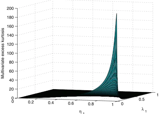
EKGM[ǫt] =K(K+2)
cess kurtosis of the Gaussian mixture distribution for K=2 andS=2,which depends only on the parametersη1 andλ1 and may increase as necessary for values ofη1andλ1close to 1 and 0, respectively.
3. INFERENCE FOR THE GAUSSIAN MIXTURE DYNAMIC CONDITIONAL CORRELATION MODEL
In this section we conduct inference for the parameters of the proposed GMDCC model by both maximum likelihood and Bayesian methods. Maximum likelihood (ML) tion has become the favorite approach for parameter estima-tion in multivariate GARCH-type models. This is obtained by maximizing the likelihood function of the model with re-spect to the model parameters. Assume first that the number of mixture components, S, is fixed. In this case the parame-ters of the GMDCC model can be summarized in the vector
=(′1, . . . ,K′ ,′,′)′, wherei=(μi, ωi, αi,1, . . . , αi,pi,
βi,2, . . . , βi,qi, δi, γi)′, for i = 1, . . . ,K, are the parameters
of the conditional volatilities of the single returns, =
(θ1, θ2,R12, . . . ,RK−1,K)′, are the parameters of the conditional correlation matrix, and =(η1, . . . , ηS−1, λ1, . . . , λS−1)′ are the parameters of the Gaussian mixture. Assuming the Gaussian
Figure 1. Multivariate excess kurtosis of the Gaussian mixture distributions forK=2 andS=2. The online version of this figure is in color.
mixture specification for the standardized innovation distribu-tion, the likelihood function of the model for the observed re-turn seriesy=(y1, . . . ,yT)is given by
where p(yt|s) is the probability density function of the Gaussian distribution with meanμand covariance matrixσs2Ht, andρs andσs2 are given in terms ofin eqs. (4) and (5), re-spectively. In practice, instead of maximizing the likelihood in eq. (6), we obtain the ML estimate of , denoted by , by maximizing the logarithm of the likelihood function,
l(|y)= −TK
Although consistency and asymptotic normality of the QMLE of different multivariate GARCH-type models have been es-tablished by several authors, deriving the consistency and the asymptotic distribution of the ML estimate for the GMDCC model is a challenging task that is beyond the scope of this article. To report standard errors of the ML estimate, we con-jecture that the usual asymptotic results for Gaussian mixtures hold in this situation and treat √T(−)as normally dis-tributed with mean 0 and covariance matrix the inverse of the expected Fisher information matrix. Consequently, the standard deviations of the estimated model parameters should be inter-preted carefully, but we present them here for completeness.
Once that the model parameters have been estimated, we may use the MLE to estimate in-sample volatilities and corre-lations and to predict future volatilities and correcorre-lations. First, obtaining estimates of in-sample volatilities and correlations is
straightforward simply by replacing by its ML estimate in
the respective equations forHt andRt, fort=1, . . . ,T. Sec-ond, given the ML estimate, predictions ofHT+1andRT+1can be obtained similar as was done in the case of in-sample esti-mation. Finally,yT+1is predicted by using the estimated mean of the process,μ.
Next, we develop a procedure for performing Bayesian infer-ence of the GMDCC model. Bayesian analysis can be greatly simplified by introducing a set of unobserved latent variables, z=(z1, . . . ,zT)′, indicating the specific component of the mix-ture from which each return is assumed to arise. Thus the so-called “complete likelihood function” for the returns and latent variables can be written as 0 otherwise. Under the Bayesian framework, inference on the parameters of the model,, can be done through the posterior density ofconditionally on the return series,y, and the latent variables,z, denoted byp(|y,z). Using the Bayes theorem,
p(|y,z)= L(|y,z)p() L(|y,z)p()d,
where p() is the prior probability of . Obviously,
ana-lytical derivation of the posterior distribution p(|y,z) for the GMDCC model becomes intractable, but we may rely on MCMC methods to obtain samples ofp(|y,z). The idea is to build an irreducible and aperiodic Markov chain in the para-meter space with states(0),(1), . . . ,(N), where(0)is the
initial state such that under very mild conditions, the chain has equilibrium distributionp(|y,z). Therefore, asngoes to infin-ity,(n)tends in distribution to a random variable with density
p(|y,z). Moreover, iff is a function of the parameters, then the strong law of large numbers guarantees that
1
almost surely, wherebis the number of realizations discarded in a burn-in period. (See, e.g., Robert and Casella2004for an overview on MCMC methods from both theoretical and practi-cal standpoints.)
First, we need to specify the expressions of the prior distri-bution,p(). We use independent uniform prior distributions in the domain of all the bounded parameters of the vector, that is, the parameters(αi,1, . . . , αi,pi)′of the EGARCH mod-els, the parameters of the correlation matrixes of the vector,
and the parameters of the Gaussian mixture of the vector .
On the other hand, we use independent normal distribution with mean 0 and a very large variance (e.g., 100) for all of the unbounded parameters of the vector, that is, the parame-ters(μi, ωi, βi,2, . . . , βi,qi, δi, γi)′of the EGARCH models. The variance of this Gaussian prior is much larger than the variance of the posterior distribution obtained, so it ensures that we are using noninformative, but proper priors for all of the model pa-rameters.
Now we construct an MCMC algorithm to sample from the posterior distributionp(|y,z). As noted by Vrontos, Della-portas, and Politis (2003a,2003b), the convergence of this type of algorithm may be accelerated by updating the highly cor-related parameters simultaneously using a block-sampling ap-proach. Thus we define the following algorithm scheme whose main steps are elaborated as follows:
1. Set n= 0 and initial values (0) =(1(0)′, . . . ,(K0)′,
In step 2 we sample from the conditional posterior proba-bilities that each multivariate return yt, for t=1, . . . ,T, has been generated from thesth component. These probabilities are given by step 3 we sample from the conditional posterior probability of
iwhose kernel is given by
κ(i|1, . . . ,i−1,i+1, . . . ,K,,,y,z) use of the random-walk Metropolis–Hastings method (RWMH) (see, e.g., Robert and Casella2004) using the following steps:
3.1. Generate a candidate vector i from the multivariate normal distribution N(i(n),ci), where cis a
con-The constant c is taken by tuning the acceptance rate to
achieve fast convergence. Usually, an acceptance rate lying be-tween 0.2 to 0.5 is plausible and practical for good convergence. Finally, in steps 4 and 5 we sample from the conditional pos-terior distributions ofand, respectively, whose kernels are given by spectively, which can be performed using a similar RWMH as that described in step 3.
Besides making inference on the parameters of the GMDCC model, we may use the Markov chain to estimate in-sample volatilities and correlations and to predict future volatilities and correlations. First, a sample from the posterior distribu-tion of each condidistribu-tional variance, Hiit, for i=1, . . . ,K and t=1, . . . ,T, can be obtained by calculating the value of each conditional variance for each draw,(n), which is denoted by
Hiit(n), forn=b+1, . . . ,T. Then the posterior expected value of
Hiit,E[Hiit|y], can be approached by the mean of the posterior sample of conditional volatilities, that is,
1
In addition, 95% Bayesian confidence intervals can be obtained by just calculating 0.025 and 0.975 quantiles of each poste-rior sample, respectively. Similarly, we can estimate in-sample correlationsRijt, using the drawsR(ijtn). A sample from the pre-dictive distribution ofHii,T+1 andRij,T+1and 95% predictive intervals can be obtained similarly to the case of in-sample es-timation. On the other hand, the predictive density of yT+1 is given by
from which we can obtain point predictions and predictive in-tervals. The prediction of Hii,T+m, Rij,T+m, and yT+m when m>1 is more complicated because the values of yt are
un-known fort≥T+1. However, we also can generate samples
from the predictive distributions ofHii,T+m,Rij,T+m, andyT+m, whenm>1, using a generalization of the sequential procedure proposed by Ausín and Galeano (2007).
Estimating the number of mixture components,S, from the
return series is a very difficult task, especially because it in-volves inference for models that may be overfitted if the true number of components is less than the number of compo-nents of the fitted model. From the frequentist standpoint, it has been widely documented that standard test theory breaks down in mixture contexts. For instance, the usual χ2 asymp-totic distribution of the likelihood ratio test statistics does not hold in mixture modeling. On the other hand, several meth-ods are available for selecting the mixture components from a Bayesian standpoint, including the use of marginal likelihoods, Bayes factors, entropy distance, or more complex approaches, such as reversible-jump MCMC algorithms or birth-and-death
processes (see Marin, Mengersen, and Robert 2005).
How-ever, a simple, plausible method frequently considered from both standpoints is the use of the Bayesian information cri-terion (BIC). In fact, the BIC has been applied by many au-thors to finite mixture models, and several simulation stud-ies support its use. Moreover, in the case of iid observations, the BIC has been found to be consistent in selecting the true number of the mixture components (see Keribin2000). In our problem, the BIC selects the number of mixture components,
S, which provides the minimum value of the BIC given by
BIC(s)= −2l(|y,s)+log(T)ms, wherel(|y,s)is the value of the log-likelihood function in eq. (7) evaluated at the ML
es-timation parameters,, assuming smixture components, and
ms is the number of parameters of the GMDCC model withs
mixture components.
4. VALUE AT RISK CALCULATION AND PORTFOLIO SELECTION
In this section we analyze two of the most important issues in risk management, namely the calculation of the VaR of a given portfolio and the portfolio selection problem, using the infor-mation provided by the proposed GMDCC model. In particu-lar, we show how to obtain point estimates of both the portfolio VaR at a given significance level and the weights of the opti-mal portfolio based on both maximum likelihood and Bayesian approaches. Using the Bayesian methodology, besides of giv-ing point estimates, we provide a measure of precision for both VaR and optimal weight estimates via predictive intervals.
Given a vector return seriesyt=(y1t, . . . ,yKt)′, a portfolio of the components ofyt, denoted bypt, is defined as a linear combination of the individual returns (i.e.,pt=δ′yt), where the weightsδ=(δ1, . . . , δK)′ add to 1. The VaR may be defined as the maximum potential loss expected with probability 1−π, whereπis supposed to be small. Statistically speaking, the one-step-ahead VaR, denoted by VaRT+1, is defined as the negative
value of the 100πth quantile of the distribution of the portfolio return, that is, Pr(pT+1≤ −VaRT+1)=π. Assuming that the model parameters are known, the conditional distribution of the one-step-ahead portfolio is
pT+1|,y∼ρ1N(δ′μ, σ12δ′HT+1δ)+ · · ·
+ρSN(δ′μ, σS2δ′HT+1δ). (11) Thus VaRT+1is the negative value of the 100πth quantile of this univariate mixture, which may be easily obtained using, for instance, the Newton–Raphson method.
Consequently, with the ML estimate of the parameters, ,
one may obtain an estimate of VaRT+1by just simply replacing
μ, σs2, and HT+1 by their respective estimates. On the other hand, using the posterior sample,(n), a consistent estimator ofE[VaRT+1|y], is given by can obtain predictive intervals for VaRT+1using the quantiles of VaR(Tn+)1, forn=b+1, . . . ,N.
Although other alternatives are plausible, to exemplify the performance of the proposed model for portfolio selection, we assume that the one-step-ahead portfolio is optimal if it has minimum VaRT+1, that is, minimum risk. Therefore, the
one-step-ahead optimal portfolio is the solution of
δopt=arg min δ {
VaRT+1:δ′1K=1}, (12)
where1K=(1, . . . ,1)′. Given δopt, the expected gain for the optimal portfolio isgopt=δ′optμ. It is well known that the so-lution of the problem in eq. (12) is not analytically tractable even under the Gaussianity assumption. However, we can make use of numerical optimization procedures to solve it. Given the distribution in eq. (11), the VaRT+1 depends onδ and. From a frequentist standpoint,is replaced by its ML estimate and the uncertainty due to parameter estimation is ignored. The
Bayesian approach allows for the inclusion of parameter uncer-tainty through the posterior distribution of. Given the sam-ples from this posterior distribution, we can obtain a sample of the posterior distribution of the optimal weights, denoted by
δ(optn), and a sample from the posterior distribution of the optimal expected gain, denoted byg(optn)=δopt(n)′μ(n). Finally, we can ob-tain consistent estimators of the posterior mean of the optimal weights and gain, respectively, using
1
N−b N
n=b+1
δ(optn) and 1
N−b N
n=b+1
g(optn).
Also, Bayesian confidence intervals can be obtained using the quantiles of the posterior samples.
5. COMPUTATIONAL ISSUES
In this section we illustrate some of the examples that we have performed to examine our proposed procedure. We con-sider three bivariate series, with sample sizesT=1,000, 2,000,
and 3,000, simulated from the GMDCC model with: (i)
indi-vidual EGARCH(1, 1) models with parameter vectors 1=
(0.05,−0.1,0.93,−0.1,0.1)′ and 2 = (0.03,−0.11,0.91, −0.12,0.11)′, (ii) dynamic conditional correlation with para-meter vector=(0.8,0.1,0.7)′, and (iii) a Gaussian mixture distribution with parameters=(0.9,0.15)′. We assume that 90% of the innovations are generated from a Gaussian dis-tribution with variance σ12≈0.64 and that 10% of the inno-vations are generated from a Gaussian mixture with variance
σ22≈4.25. This second mixture component is designed to con-tain the extremes.
First, for each of the simulated series, we obtain the ML es-timate of the model parameters for S=1, . . . ,5 components
Table 1. Computed values of the BIC for each simulated series for
S=1, . . . ,5 mixture components
BIC T=1,000 T=2,000 T=3,000
S=1 2,566.0 5,327.4 7,726.8
S=2 2,399.0 4,819.6 6,833.4
S=3 2,412.8 4,834.8 6,848.4
S=4 2,426.6 4,850.0 6,864.4
S=5 2,440.4 4,865.2 6,880.4
of the mixture as described in Section3. We then compute the values of the BIC for each simulated series, as shown in Ta-ble1. In every case, the BIC selects the true valueS=2 mixture
components. Then, assuming thatS=2, we run the proposed
MCMC algorithm for each simulated series using 20,000 iter-ations and discard the initial 10,000 iterations for inference as burn-in iterations. We consider the ML estimate of the parame-ters as the initial values and use the block-sampling approach
described in Section3. The MCMC chains provide good
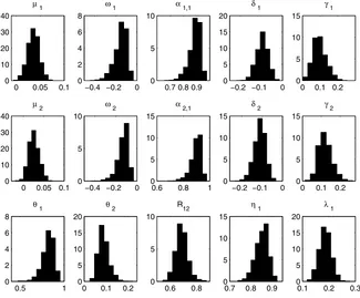
mix-ing performance and fast convergence. Figure2shows the his-tograms of the posterior samples of each model parameter for the first simulated series with sample sizeT=1,000. We see that the algorithm captures the asymmetry of the posterior dis-tributions of the parametersω1, α1,1, ω2, α2,1, θ1, andθ2. We also observed that, as expected, these posterior distributions be-came more symmetric forT=2,000 andT=3,000 (data not reported).
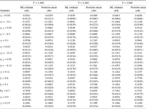
Table2compares the ML estimates and standard errors with the Bayesian posterior means and standard deviations of the model parameters for the three simulated series. Note that both approaches lead to similar point estimates and that in general, the posterior standard deviations are larger than the standard errors when the posterior distributions are asymmetric. This is
Figure 2. Histograms of the posterior MCMC samples of each model parameter corresponding to the first simulated series withT=1,000. The online version of this figure is in color.
Table 2. Maximum likelihood and Bayesian estimates of the model parameters for the three simulated series
T=1,000 T=2,000 T=3,000
ML estimate Posterior mean ML estimate Posterior mean ML estimate Posterior mean
Parameter (std) (std) (std) (std) (std) (std)
μ1=0.05 0.0361 0.0359 0.0359 0.0369 0.0463 0.0456
(0.0123) (0.0121) (0.0089) (0.0087) (0.0066) (0.0066) ω1= −0.1 −0.1077 −0.1551 −0.0991 −0.1137 −0.1068 −0.1130
(0.0424) (0.0588) (0.0255) (0.0273) (0.0184) (0.0189) α1,1=0.93 0.9225 0.8866 0.9249 0.9130 0.9198 0.9143
(0.0296) (0.0433) (0.0190) (0.0206) (0.0135) (0.0143) δ1= −0.1 −0.0884 −0.0967 −0.0960 −0.0969 −0.1109 −0.1138
(0.0241) (0.0274) (0.0174) (0.0182) (0.0122) (0.0133) γ1=0.1 0.0708 0.0974 0.1120 0.1243 0.0919 0.0961
(0.0327) (0.0384) (0.0248) (0.0256) (0.0159) (0.0160) μ2=0.03 0.0247 0.0254 0.0226 0.0237 0.0344 0.0342
(0.0131) (0.0126) (0.0093) (0.0083) (0.0072) (0.0071) ω2= −0.11 −0.0931 −0.1330 −0.1055 −0.1163 −0.1151 −0.1231
(0.0313) (0.0517) (0.0224) (0.0233) (0.0215) (0.0216) α2,1=0.91 0.9278 0.8952 0.9103 0.9002 0.8970 0.8892
(0.0241) (0.0403) (0.0182) (0.0187) (0.0182) (0.0181) δ2= −0.12 −0.0968 −0.1120 −0.1213 −0.1261 −0.1079 −0.1094
(0.0244) (0.0285) (0.0170) (0.0175) (0.0145) (0.0148) γ2=0.11 0.0987 0.1198 0.1033 0.1140 0.1264 0.1337
(0.0330) (0.0357) (0.0247) (0.0246) (0.0198) (0.0209) θ1=0.8 0.8522 0.8156 0.8307 0.8190 0.7879 0.7799
(0.0409) (0.0662) (0.0345) (0.0363) (0.0265) (0.0265) θ2=0.1 0.0761 0.0885 0.0743 0.0768 0.1044 0.1070
(0.0183) (0.0245) (0.0136) (0.0140) (0.0126) (0.0126)
R12=0.7 0.7039 0.6874 0.6983 0.6935 0.7382 0.7351
(0.0407) (0.0460) (0.0243) (0.0241) (0.0181) (0.0175) η1=0.9 0.8543 0.8522 0.9055 0.9015 0.9076 0.9062
(0.0338) (0.0308) (0.0134) (0.0130) (0.0104) (0.0109) λ1=0.15 0.1881 0.1860 0.1379 0.1399 0.1286 0.1289
(0.0286) (0.0225) (0.0155) (0.0134) (0.0105) (0.0102)
caused by the asymptotic Gaussian assumption of the ML esti-mate. However, as expected, the standard errors and posterior standard deviations become smaller and more similar as the sample size, T, increases. Finally, besides providing point es-timates and standard errors, the Bayesian estimation also pro-duces posterior densities that describe all of their uncertainty associated with the model parameters. Moreover, this uncer-tainty may be introduced in the estimation of volatilities, cor-relations, VaR, portfolio selection, and so on, as we show later. Next, we estimate the in-sample volatilities and correlations using both ML estimates and the Bayesian approaches. This is illustrated in Figure3, which presents the estimated in-sample volatilities,Hiit, fori=1,2, and the estimated in-sample corre-lations,R12t, fort=1,900, . . . ,2,000, for the second simulated series with sample size T=2,000 are presented. Also shown are 95% Bayesian confidence intervals and true values. Observe the accuracy of the estimations and note that the Bayesian con-fidence intervals always include the true values ofHiit andR12t for all time periods. We also can make predictions of future volatilities and correlations as shown in Figure3, which shows the point estimations and Bayesian intervals for the one-step-ahead volatilities,Hii,T+1, fori=1,2, and correlation,R12,T+1,
whereT+1=2,001, and compares them with their true values.
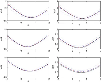
We next apply the procedures described in Section4for VaR calculation and portfolio selection. Figure4shows the ML and Bayesian estimations for the one-step-ahead VaRT+1 of port-folios of the formpT+1=δ×y1,T+1+(1−δ)×y2,T+1, as
a function ofδ,for the three simulated series and forπ=0.05 andπ=0.01. Also shown are the Bayesian 95% confidence in-tervals and true values. Observe the accuracy of the estimations and note that the Bayesian confidence intervals always include the true VaRT+1values. In contrast, Table3gives the maximum likelihood and Bayesian estimations of the optimal weight,δopt, of the portfolio pT+1=δopt ×y1,T+1+(1−δopt)×y2,T+1,
which minimizes the one-step-ahead VaRT+1, and the
corre-sponding optimal gain,gopt, for the three simulated series. Also shown are the Bayesian 95% confidence intervals and true val-ues. Note that the obtained optimal weights are coherent with the plots shown in Figure4.
Finally, we also performed simulations with
larger-dimen-sional systems in whichK=5 and K=10. In the cases, the
only problem found is that the greater computational cost of obtaining both ML and Bayesian estimates compared with that required for smaller systems. Apparently, the accuracy of the estimates is not significantly affected by large dimensions, how-ever.
Figure 3. True (solid), ML (dashed), and Bayesian (dashed–dotted) estimates and 95% predictive intervals (dotted) for the volatilities,Hiit,
fori=1,2, and correlations,R12t, fort=1,900, . . . ,2,001, for the second simulated series with sample sizeT=2,000. The online version of
this figure is in color.
6. APPLICATION
As an illustration, we apply the proposed methodology to the daily closing prices of Dow Jones Industrial Average and
NASDAQ composite indexes for the period January 2, 1996 to December 29, 2006. The log return series of sample size
T=2,769 is affected by the presence of several extremes. The sample means, variances, and excess kurtosis of the two
log-Figure 4. True (solid), ML (dashed), and Bayesian (dashed–dotted) estimates and 95% predictive intervals (dotted) for the VaRT+1of the
portfoliopT+1=δ×y1,T+1+(1−δ)×y2,T+1as a function ofδ,for the series withT=1,000 (top), 2,000 (middle), and 3,000 (bottom) and
forπ=0.05 (left) andπ=0.01 (right). The online version of this figure is in color.
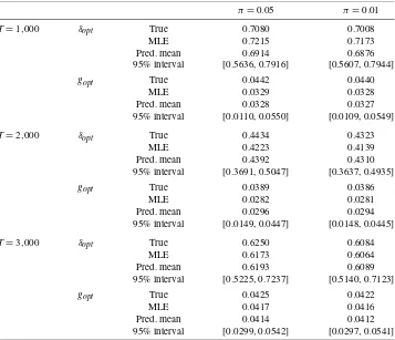
Table 3. True values and ML and Bayesian point estimates together with 95% predictive intervals for the optimal weight,δopt,of the optimal portfolioδopt,1×y1,T+1+(1−δopt,1)×y2,T+1,
and for the corresponding expected gain, for the three simulated series
π=0.05 π=0.01
T=1,000 δopt True 0.7080 0.7008
MLE 0.7215 0.7173
Pred. mean 0.6914 0.6876 95% interval [0.5636, 0.7916] [0.5607, 0.7944]
gopt True 0.0442 0.0440
MLE 0.0329 0.0328
Pred. mean 0.0328 0.0327 95% interval [0.0110, 0.0550] [0.0109, 0.0549]
T=2,000 δopt True 0.4434 0.4323
MLE 0.4223 0.4139
Pred. mean 0.4392 0.4310 95% interval [0.3691, 0.5047] [0.3637, 0.4935]
gopt True 0.0389 0.0386
MLE 0.0282 0.0281
Pred. mean 0.0296 0.0294 95% interval [0.0149, 0.0447] [0.0148, 0.0445]
T=3,000 δopt True 0.6250 0.6084
MLE 0.6173 0.6064
Pred. mean 0.6193 0.6089 95% interval [0.5225,0.7237] [0.5140,0.7123]
gopt True 0.0425 0.0422
MLE 0.0417 0.0416
Pred. mean 0.0414 0.0412 95% interval [0.0299,0.0542] [0.0297,0.0541]
return series are 0.0317 and 0.0297, 1.1833 and 3.1013, and 4.178 and 4.182, respectively. The autocorrelation functions of both returns show no significant autocorrelations. In fact, the Ljung–Box statistics for both log returns for lag 5 are 7.987 and 13.375,and those for lag 10 are 109.480 and 13.688, with associated p-values of 0.157 and 0.203, and 0.091 and 0.188, respectively. The sample correlation between both log returns is 0.705.
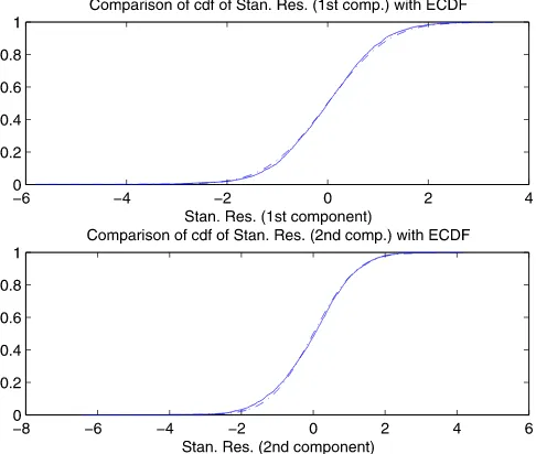
First, we estimate the GMDCC model using both ML and the Bayesian procedure. We obtain the ML estimates of the model parameters forS=1, . . . ,4 and compute the value of the BIC. These are given by 1.5016×10⁴, 1.4939×10⁴, 1.4943×10⁴, and 1.4959×10⁴. Therefore, the BIC selectsS=2 components in the mixture. Table4gives the ML estimates of the model pa-rameters forS=2. Figure5compares the empirical cumulative distribution function of the standardized residuals with the cu-mulative distribution function of the estimated Gaussian mix-ture, showing a good fit. In fact, the Kolmogorov–Smirnov test does not reject the null hypothesis of equality of distributions for significance levelsα=0.05 andα=0.01. Then, we run the proposed MCMC algorithm for the bivariate series with 20,000 iterations, using the first 10,000 as burn-in iterations. Table4
also gives the posterior means and standard deviations obtained from the MCMC output, leading to similar results as for ML es-timation. Both approaches predict that about 97% of the innova-tions are generated by the mixture component with smaller co-variance matrix, whereas approximately the 3% are generated by the component with larger covariance matrix. In addition,
the covariance matrix of this second component, which may be viewed as the component with the extremes, is estimated to be approximately 4.5 times larger than the smaller covariance ma-trix.
Figure6illustrates the ML and Bayesian estimates together with 95% Bayesian confidence intervals for the volatilities,Hiit, fori=1,2, and correlations,R12t, of the last 100 returns. The ML estimates are very close to the Bayesian posterior means for
Table 4. ML and Bayesian estimates of the model parameters for the Dow Jones and NASDAQ indexes
μ1 ω1 α1,1 δ1 γ1
MLE 0.0412 0.0023 0.9908 −0.0322 0.0952 (std) (0.0139) (0.0013) (0.0021) (0.0069) (0.0101) Post. mean 0.0479 0.0024 0.9900 −0.0342 0.1020 (std) (0.0139) (0.0016) (0.0024) (0.0082) (0.0119)
μ2 ω2 α2,1 δ2 γ2
MLE 0.0562 −0.0003 0.9941 −0.0147 0.0929 (std) (0.0199) (0.0014) (0.0016) (0.0059) (0.0111) Post. mean 0.0661 −0.0001 0.9936 −0.0152 0.0999 (std) (0.0184) (0.0016) (0.0017) (0.0062) (0.0109)
θ1 θ2 R12 η1 λ1
MLE 0.9711 0.0148 0.8704 0.9741 0.2134 (std) (0.0067) (0.0032) (0.0231) (0.0102) (0.0327) Post. mean 0.9667 0.0164 0.8651 0.9607 0.2443 (std) (0.0087) (0.0040) (0.0210) (0.0228) (0.0579)
Figure 5. Empirical cumulative distribution function of the stan-dardized residuals compared with the cumulative distribution function of the Gaussian mixture with parametersρ1andλ1estimated by ML
estimation for the GMDCC model. The online version of this figure is in color.
the all time periods. Note that the Bayesian confidence intervals ofH11t,H22t, andR12tare not necessarily symmetric. Figure6 also includes the one-step-ahead point predictions ofHii,2,770,
fori=1,2, and the correlation, R12,2,770, along with the
cor-responding predictive intervals. It appears that the NASDAQ index is more volatile than the Dow Jones index in this last pe-riod of 2006. In fact, this effect was seen since 1998 (data not
reported). Also note that the conditional correlations are very high, with values around 0.9 and a drop at the end of November 2006.
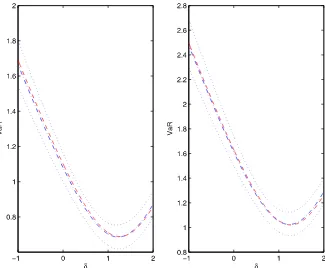
Figure 7illustrates both ML and Bayesian estimates along
with 95% confidence intervals for the one-step-ahead VaRT+1
of the portfolio pT+1 = δ × DowJonesT+1 + (1 − δ) ×
NasdaqT+1, forδ∈(−1,2), andπ=0.05 andπ=0.01. Ob-serve that the Bayesian confidence intervals always include the
ML estimate for each weightδ. The one-step-ahead VaR
mimizing portfolio weight seems to outweigh the Dow Jones in-dex. This effect can be clearly seen in Table 5, which gives both the ML and Bayesian estimates with a 95% predictive interval for the optimal weight, δopt, of the optimal portfo-lio,δopt,1DowJonesT+1+(1−δopt,1)NasdaqT+1,and the cor-responding expected gain, gopt, for π =0.05 and π =0.01. Both approaches predict an optimal portfolio weight of approx-imately 1.25 on the Dow Jones index. Finally, note that the gains from using the optimal portfolio weight are statistically significant.
7. CONCLUSIONS
In this article we have proposed a multivariate GARCH model with time-varying correlations in which the individual conditional volatilities follow a univariate EGARCH model and the standardized innovations are assumed to follow a mixture of multivariate zero mean Gaussian distributions. This speci-fication extends the Gaussian mixture innovation distribution proposed by Bai, Rusell, and Tiao (2003) to the multivariate framework with an unknown number of mixture components. We have shown how to perform both ML and Bayesian infer-ence on this model. In particular, Bayesian inferinfer-ence is done using MCMC methods, allowing estimation and prediction of
Figure 6. Bayesian estimates (dashed) and 95% intervals (dotted) compared with ML estimates (dashed–dotted) for the volatilities,Hiit, for i=1,2, and correlations,R12t, of the last 100 observations for the Dow Jones and NASDAQ indexes. The online version of this figure is in
color.
Figure 7. ML (dashed) and Bayesian (dashed–dotted) estimates and 95% predictive intervals (dotted) for the VaRT+1 of the portfolio
pT+1=δ×DowJonesT+1+(1−δ)×NasdaqT+1,as a function ofδ,forπ=0.05 (left) andπ=0.01 (right). The online version of this
figure is in color.
conditional volatilities and correlations. The two approaches perform similarly, and both have been shown to work well with both simulated and real data examples. We also have developed a procedure for deriving predictive distributions for the lio VaR, as well as a method for determining optimal portfo-lios.
ACKNOWLEDGMENTS
The authors thank the editor, the associate editor, and an anonymous referee for their many helpful suggestions, which led to a much-improved article. The work of Galeano was supported by MEC project MTM2008-03010 and Xunta de Galicia project PGIDIT06PXIB207009PR. The work of Con-cepción Ausín was supported by MEC project MTM2008-00166.
[Received September 2007. Revised December 2008.]
Table 5. ML and Bayesian estimates for the weight,δopt,
and expected gain,gopt, of the optimal portfolio, δoptDowJonesT+1+(1−δopt)NasdaqT+1,
joint with 95% predictive intervals
π=0.05 π=0.01
δopt MLE 1.2589 1.2659
Pred. mean 1.2232 1.2316 95% interval [1.1430,1.2929] [1.1572,1.2983]
gopt MLE 0.0373 0.0372
Pred. mean 0.0440 0.0438 95% interval [0.0159,0.0721] [0.0156,0.0720]
REFERENCES
Ausín, M. C., and Galeano, P. (2007), “Bayesian Estimation of the Gaussian Mixture GARCH Model,”Computational Statistics and Data Analysis, 51, 2636–2652. [559,564]
Bai, X., Rusell, J. R., and Tiao, G. C. (2003), “Kurtosis of GARCH and Stochas-tic Volatility Models With Non-Normal Innovations,”Journal of Economet-rics, 114, 349–360. [559,561,569]
Bauwens, L., Hafner, C. M., and Rombouts, J. V. K. (2007), “Multivariate Mixed Normal Conditional Heteroskedaticity,” Computational Statistics and Data Analysis, 51, 3551–3566. [559]
Bauwens, L., Laurent, S., and Rombouts, J. V. K. (2006), “Multivariate GARCH Models: A Survey,”Journal of Applied Econometrics, 21, 79–109. [559,560]
Bollerslev, T. (1986), “Generalized Autoregressive Conditional Heteroskedas-ticity,”Journal of Econometrics, 31, 307–327. [559]
(1990), “Modelling the Coherence in Short-Run Nominal Exchange Rates: A Multivariate Generalized ARCH Model,”Review of Economics and Statistics, 72, 498–505. [559]
Bollerslev, T., and Engle, R. F. (1993), “Common Persistence in Conditional Variances,”Econometrica, 61, 167–186. [559]
Bollerslev, T., Engle, R. F., and Wooldridge, J. M. (1988), “A Capital Asset Pricing Model With Time-Varying Covariances,”Journal of Political Econ-omy, 96, 116–131. [559]
Engle, R. F. (1982), “Autoregressive Conditional Heteroskedasticity With Esti-mates of the Variance of the U.K. Inflation,”Econometrica, 50, 987–1008. [559]
(2002), “Dynamic Conditional Correlation: A Simple Class of Mul-tivariate Generalized Autoregressive Conditional Heteroskedasticity Mod-els,”Journal of Business & Economic Statistics, 20, 339–350. [559] Engle, R. F., and Kroner, K. (1995), “Multivariate Simultaneous GARCH,”
Econometric Theory, 11, 122–150. [559]
Engle, R. F., Ng, V. K., and Rothschild, M. (1990), “Asset Pricing With a Fac-tor ARCH Covariance Structure: Empirical Estimates for Treasury Bills,” Journal of Econometrics, 45, 213–238. [559]
Frühwirth-Schnatter, S. (2006),Finite Mixture and Markov Switching Models, New York: Springer. [561]
Haas, M., Mittnik, S., and Paolella, M. S. (2004), “Mixed Normal Conditional Heteroskedasticity,”Journal of Financial Econometrics, 2, 211–250. [559] Hall, P., and Yao, Q. (2003), “Inference in ARCH and GARCH Models With
Heavy-Tailed Errors,”Econometrica, 71, 285–317. [561]
Jeantheau, T. (1998), “Strong Consistency of Estimators for Multivariate ARCH Models,”Econometric Theory, 14, 70–86. [561]
Keribin, C. (2000), “Consistent Estimation of the Order of Mixture Models,” Sankhya, Ser. A, 62, 49–66. [564]
Kroner, F. K., and Ng, V. K. (1998), “Modelling Asymmetric Comovements of Asset Returns,”The Review of Financial Studies, 11, 817–844. [559] Mardia, K. V. (1970), “Measures of Multivariate Skewness and Kurtosis With
Applications,”Biometrika, 57, 519–530. [561]
Marin, J.-M., Mengersen, K. L., and Robert, C. P. (2005), “Bayesian Modelling and Inference on Mixtures of Distributions,” inBayesian Modelling and Inference on Mixtures of Distributions. Handbook of Statistics, Vol. 25, eds. D. Dey and C. R. Rao, Amsterdam: North-Holland. [564]
Markowitz, H. (1952), “Portfolio Selection,”Journal of Finance, 8, 77–91. [560]
Nelson, D. B. (1991), “Conditional Heteroskedasticity in Asset Returns: A New Approach,”Econometrica, 59, 347–370. [559,560]
Perez-Quiros, G., and Timmermann, A. (2000), “Firm Size and Cyclical Varia-tions in Stock Returns,”The Journal of Finance, 55, 1229–1262. [559]
(2001), “Business Cycle Asymmetries in Stock Returns: Evidence From Higher Order Moments and Conditional Densities,” Journal of Econometrics, 103, 259–306. [559]
Robert, C. P., and Casella, G. (2004),Monte Carlo Statistical Methods(2nd ed.), New York: Springer. [563]
Tse, Y. K., and Tsui, A. K. C. (2002), “A Multivariate Generalized Au-toregressive Conditional Heteroscedasticity Model With Time-Varying Correlations,”Journal of Business & Economic Statistics, 20, 351–362. [559,560]
Vrontos, I. D., Dellaportas, P., and Politis, D. N. (2003a), “A Full-Factor Mul-tivariate GARCH Model,”Econometrics Journal, 6, 312–334. [559,563]
(2003b), “Inference for Some Multivariate ARCH and GARCH Mod-els,”Journal of Forecasting, 22, 427–446. [559,563]
Wong, C., and Li, W. (2001), “On a Mixture Autoregressive Conditional Het-eroscedastic Model,”Journal of the American Statistical Association, 96, 982–995. [559]