Full Terms & Conditions of access and use can be found at
http://www.tandfonline.com/action/journalInformation?journalCode=ubes20
Download by: [Universitas Maritim Raja Ali Haji] Date: 12 January 2016, At: 17:42
Journal of Business & Economic Statistics
ISSN: 0735-0015 (Print) 1537-2707 (Online) Journal homepage: http://www.tandfonline.com/loi/ubes20
Bayesian Analysis of the Output Gap
Christophe Planas, Alessandro Rossi & Gabriele Fiorentini
To cite this article: Christophe Planas, Alessandro Rossi & Gabriele Fiorentini (2008) Bayesian
Analysis of the Output Gap, Journal of Business & Economic Statistics, 26:1, 18-32, DOI: 10.1198/073500106000000576
To link to this article: http://dx.doi.org/10.1198/073500106000000576
Published online: 01 Jan 2012.
Submit your article to this journal
Article views: 103
View related articles
Bayesian Analysis of the Output Gap
Christophe P
LANASJoint Research Centre, European Commission, 21020 Ispra (VA), Italy (christophe.planas@jrc.it)
Alessandro R
OSSIJoint Research Centre, European Commission, 21020 Ispra (VA), Italy (alessandro.rossi@jrc.it)
Gabriele F
IORENTINIDepartment of Statistics, University of Florence, 50134 Florence (FI), Italy (fiorentini@ds.unifi.it)
Our objective is to build output gap estimates that benefit from information provided by Phillips curve theory and business cycle studies. For this, we develop a Bayesian analysis of the bivariate Phillips curve model proposed by Kuttner for estimating potential output. Given our priors, we obtain samples from parameters and state variables joint posterior distribution following a Gibbs sampling strategy. We sample the state variables given parameters using the Carter–Kohn procedure, and we exploit a likelihood factor-ization to draw parameters given the state. A Metropolis–Hastings step is used to remove the conditioning on starting values. To accommodate the variance moderation that has been observed on U.S. gross domes-tic product, Kuttner’s model is extended for a change in variance parameters. We apply this methodology to the analysis of the output gap in the United States and in the European Monetary Union. Finally, some important extensions to the original Kuttner model are discussed.
KEY WORDS: Business cycle; Gibbs sampling; Kalman filter and smoothing; Markov chain Monte Carlo; Unobserved components.
1. INTRODUCTION
In this article we develop a Bayesian analysis of the Phillips curve bivariate model put forward by Kuttner (1994) for esti-mating the potential output and the output gap. Potential output and output gap are two concepts that are essential to macroeco-nomic analysis because they are related to different ecomacroeco-nomic forces: potential output measures long-term movements asso-ciated with steady economic growth, whereas the output gap captures all short-term fluctuations (see, for instance, Hall and Taylor 1991). The concurrent output gap is, hence, subject to careful monitoring by institutions responsible for stabilization policy and inflation control. Taylor (1993) acknowledged this when building his famous rule for describing the Federal Re-serve monetary policy.
Kuttner’s (1994) original model relates output gap to infla-tion through the Phillips curve. Although somewhat atypical because it involves a regression on an unobserved variable, this model has entertained a certain success. For instance, Kichian (1999) applied it to the G7 countries, Gerlach and Smets (1999) emphasized its appeal for the European Central Bank policy-making process, and Apel and Jansson (1999a, b) further ex-tended it to include unemployment. The European Commission uses this framework for estimating structural unemployment (see Planas, Roeger, and Rossi 2007), whereas the NAIRU es-timates of the Organization of Economic Cooperation and De-velopment (OECD) are obtained from a closely related model (see OECD 2000).
In this particular context of cycle estimation embedded into a Phillips curve regression, an important amount of macroeco-nomic theory and business cycle knowledge is available. It is, thus, natural to develop a Bayesian analysis in order to in-corporate this information into the decomposition. This yields several benefits. First, because Bayesian methods deliver sam-ples from posterior distributions, the finite-sample uncertainty around any quantity of interest can be precisely delineated. This
is important information: Output gap measurements have in-deed been strongly criticized for lacking reliability (see Or-phanides and van Norden 2002), and knowing the uncertainty has become imperative for policy. Second, the insertion of ad-ditional knowledge into the decomposition is expected to make Bayesian gap estimates more precise than maximum likelihood ones. In any case, researchers seeking to reduce the uncertainty can use the Bayesian framework to assess the added value of any extra information. Third, the Bayesian setting helps in un-derstanding the salient features of Phillips curve regressions: For instance, the sharpness of the response of inflation to dif-ferent proxies for detrended output can be compared (see Gali, Gertler, and Lopez-Salido 2001). Finally, by properly tuning the prior distribution of variance parameters, the pile-up prob-lem sometimes faced in classical analysis can be avoided. The pile-up problem—that is, obtaining zero variance estimates for the innovations in unobservables even though the true variance is strictly positive (see Stock and Watson 1998)—is generally undesirable because the related variable turns out deterministic and, hence, observed.
Given priors on model parameters, we implement a Gibbs sampling scheme for drawing model parameters and state vari-ables from their joint posterior distribution (see, for instance, Casella and George 1992 and the general discussion in Geweke 1999). We sample the state conditionally on parameters on the basis of the Carter–Kohn (1994) sampler with de Jong’s (1991) Kalman filter initialization. We draw the state in its first time period using the results in Koopman (1997). A likelihood fac-torization allows us to sample the parameters given the state in three blocks. We also introduce Metropolis–Hastings steps (see, for instance, Chib and Greenberg 1995) for removing the conditioning on the first observations. We reparameterize
© 2008 American Statistical Association Journal of Business & Economic Statistics January 2008, Vol. 26, No. 1 DOI 10.1198/073500106000000576
18
the traditional cyclical AR(2) model in terms of polar coordi-nates of the characteristic equation roots. We find this neces-sary mainly because specifying diffuse priors for autoregres-sive parameters implies informative priors on periodicity and amplitude. We then resort to the adaptive rejection Metropolis method proposed by Gilks, Best, and Tan (1995) for sampling the polar coordinates (see also the corrigendum by Gilks, Neal, Best, and Tan 1997). We also reparameterize the covariance be-tween shocks in inflation and in the gap. Finally, in order to ac-commodate the variance moderation that has been observed on U.S. gross domestic product (GDP) (see Kim and Nelson 1999; McConnell and Perez-Quiros 2000; Stock and Watson 2002), we extend Kuttner’s original model to allow for a break in the variance parameters. Our empirical results suggest that the sam-pling scheme we put forward produces low correlations in the chain, for a greater efficiency of posterior density estimates.
Section 2 discusses the model structure, the parameteriza-tion adopted, and the prior distribuparameteriza-tions. Secparameteriza-tion 3 describes the procedure we propose for sampling from the joint posterior dis-tribution of both model parameters and unobserved variables in Kuttner’s model, with the possibility of a variance break. Section 4 presents an application to the 12 countries of the European Monetary Union (EMU) and to the United States. Several model extensions together with their Bayesian treat-ment are discussed in Section 5. Section 6 concludes.
2. MODEL SPECIFICATION
Let yt denote the logarithm of real output. Like Watson (1986) and Clark (1987), we assume that it is made up of a trend,pt, and of a cycle,ct, according to
yt=pt+ct,
pt=μp+apt, (2.1)
φc(L)ct=act,
whereLis the lag operator,≡1−Lrepresents the first dif-ference,μpis a constant drift, andφc(L)=1−φc1L−φc2L2
is an AR(2) polynomial with stationary and complex roots. The permanent and transitory shocks, apt and act, are orthogonal Gaussian white noises with variancesVpandVc. The long-term and short-term components,ptandct, are interpreted as poten-tial output and output gap.
Kuttner (1994) complemented (2.1) with an equation that dy-namically links change in inflation, sayπt, to the output gap as in
φπ(L)πt=μπ+βct−1+λyt−1+a∗πt, (2.2) wherea∗πtis a Gaussian white noise and the roots of the AR(2) polynomialφπ(L)=1−φπ1L−φπ2L2are assumed to be
sta-tionary. The original model included a moving average instead of autoregressive terms: We make this slight modification in order to simplify the statistical analysis. Equation (2.2) intro-duces a Phillips curve effect by relating the change in inflation to the real output growth and to the latent cycle, both with one lag. As in Kuttner’s model, the innovations in inflation and in the gap are assumed contemporaneously correlated, with corre-lation coefficientρcπ. Letκπ denote a real parameter and let
aπt be a Gaussian white noise with variance Vπ orthogonal
toact. We reparameterize ρcπ by writing the innovationsa∗πt
the Bayesian treatment of all parameters homogeneous. The shocksaπtandaptare assumed to be independent.
In the Bayesian framework, incorporating the prior informa-tion available often requires a careful model parameterizainforma-tion. For instance, thanks to the bulk of empirical studies, it is gener-ally admitted that business cycles in G7 countries typicgener-ally last from 2 to 10 years. Hence, we reparameterize the model for the cycle as in
1−2Acos(2π/τ )L+A2L2ct=act, (2.4) where the parametersAandτ represent the amplitude and peri-odicity of the cyclical movements, respectively. By construc-tion, these parameters describe cycles much more naturally than AR coefficients. Indeed, assuming a normal prior distrib-ution for(φc1, φc2), we found it difficult to reproduce our prior
knowledge by tuning the mean and the covariance matrix of the autoregressive parameters. And in some cases the implied distribution for the periodicity and amplitude can be counter-intuitive. Let us consider, for instance, a flat prior for the AR parameters over the region of stationary and complex roots, that is,φc21<−4φc2andφc2∈(−1,0). Half of the complex
re-gion whereφ1is negative yields roots with periodicity in[2,4],
whereas the other half yields roots with periodicity in [4,∞). Therefore, the associated distribution forτputs equal weight on the intervals[2,4]and[4,∞)and 4 is the median value. A sim-ilar reasoning suggests that the flat prior on the complex roots overweights close-to-one amplitudes. Hence, being noninfor-mative on the coefficients of AR polynomials with complex and stationary roots amounts to emphasizing short-term and persis-tent fluctuations. Putting the prior on the AR coefficients as, for instance, in Chib (1993), Chib and Greenberg (1994), or McCulloch and Tsay (1994), or on the partial autocorrelations as in Barnett, Kohn, and Sheater (1996) and in Billio, Monfort, and Robert (1999) is probably inadequate for cyclical analy-sis. The trigonometric specification proposed by Harvey (1981, pp. 182–183) and used in a Bayesian setting in Harvey, Trimbur, and van Dijk (2002) appears instead better suited. Here we stick to Kuttner’s original model by considering the polar coordinate setting (2.4). This parameterization actually simplifies Harvey’s specification by excluding a moving-average term. For a similar discussion about the link between prior and parameterizations in the local level model, see appendix C of Koop and van Dijk (2000).
We now complete the model by specifying the prior distribu-tion of all parameters. Letδ=(μπ, β, λ, φπ1, φπ2, κπ)denote
the vector of conditional mean parameters in (2.3). We shall consider the block independence structure:
p(Vc)=IG(sc0,vc0),
p(δ,Vπ)=NIG(δ0,Mδ−1,sπ0,vπ0)Iδ,
p(μp,Vp)=NIG(μp0,Mp−01,sp0,vp0),
where Beta(·,·)is the Beta distribution,τlandτuare the lower and upper bounds ofτ’s support, IG(·)is the inverted Gamma distribution, NIG(·) is the Normal-inverted Gamma distribu-tion, andIδis an index set for imposing constraints on the
pa-rameter support. The hyperpapa-rameters τl, τu, aA, bA, aτ,bτ,
δ0(6×1),Mδ (6×6),μp0,Mp0,sc0,vc0,sπ0,vπ0,sp0, and vp0 are assumed to be given; we shall discuss the setting of
some of them in the empirical application. In (2.5), the prior distributions for Vc, δ,Vπ, μp, andVp are naturally conjugate for the full conditionals of interest. Computational convenience is the main reason for this choice. The framework that en-sues, however, remains quite flexible because we can be as (non)informative as desired by properly tuning the hyperpara-meters: For instance, setting Mp0,sp0, and vp0 to small
quan-tities leads top(μp,Vp)∝1/Vp. The conjugate property is in-stead lost for the parametersAandτ. We will pay this price for the parameterization given in (2.4) in terms of computational complexity.
Letθdenote the full set of parameters, that is,θ≡(A, τ,Vc, δ,Vπ, μp,Vp). Our objective is to characterize the joint poste-rior distribution of the potential output, the output gap, and the parameters conditionally on the data, that is,p(cT,pT, θ|YT), wherexTk ≡ {xk, . . . ,xT},xT ≡xT1, andYT≡ {yT, πT}. Given
our model, no closed-form expression for this posterior is avail-able but draws from p(cT,pT, θ|YT)can be obtained using a Gibbs sampling scheme. The full conditionals of interest are
• p(cT,pT|θ,YT);
• p(θ|cT,pT,YT).
We explain how to sample from these two distributions in the next section.
3. JOINT POSTERIOR DISTRIBUTION OF STATES AND MODEL PARAMETERS
3.1 Sampling the State Variables Given Model Parameters
We first focus on simulating the unobservable components conditionally on model parameters. It will be useful to cast equations (2.1), (2.3), and (2.4) into a state space format (see, for instance, Durbin and Koopman 2001) such that
Yt=Hξt,
ξt+1=D+Fξt+wt+1,
whereYt=(yt, πt)′ is the vector of observations,ξt=(pt,ct,
ct−1, κπact +aπt)′ is the state vector, and wt =(apt,act,0, κπact+aπt)′ is a Gaussian error vector with zero mean and singular variance matrixQ. The time-invariant matricesH,D,
F, and Q can be straightforwardly recovered. As usual, ξt|k andPt|k denote the conditional expectation E(ξt|Yk)and vari-anceV(ξt|Yk). Samples fromp(cT,pT|θ,YT)will be obtained
throughp(ξT|θ,YT). We make use of the following identity that gives the basis of the Carter–Kohn (1994) state sampler:
p(ξT|θ,YT)=p(ξT|θ,YT) T−1
t=2
p(ξt|θ,Yt, ξt+1)p(ξ1|θ,Y1, ξ2),
where the last term is isolated because initial conditions need a special treatment. A draw fromp(ξT|θ,YT)can be obtained as
Steps 1 and 2 only involve classical results. Step 3 needs the conditional moments E[ξt|θ, ξt+1,Yt]andV[ξt|θ, ξt+1,Yt].
From the joint distribution of ξt and ξt+1 conditional on θ
andYt, we get
E[ξt|θ, ξt+1,Yt] =ξt|t+Pt|tF′P−t+11|t(ξt+1−Fξt|t),
V[ξt|θ, ξt+1,Yt] =Pt|t−Pt|tF′Pt−+11|tFPt|t.
Step 4 is more complicated. Fort=1, the preceding formula in-volvesξ1|1andP1|1but none of them is available in our model.
This occurs because ifd is the state integration order, that is,
d=1 in our case, the first state estimate that de Jong’s algo-rithm yields isξd+1|d. A procedure based on Koopman (1997)
for obtainingξ1|1andP1|1is detailed in Appendix A. In our
par-ticular context, use could be made of the fact thatξ2containsc1
for skipping the sampling ofξ1|1, but such a simplification only
holds when the trend integration order is 1, an assumption that will be relaxed in Section 5. The algorithm in Appendix A has the advantage of generality.
Because of the model structure, not all elements of the state need to be simulated. Trivially, givenyt, knowledge ofct deter-minespt. Also, given model parameters and observations up to timet, samplingct−1yields the last state’s element,κπact+aπt, through (2.3). We, thus, end up withct−1as the only random
el-ement to simulate at every time period. In this situation, using a more efficient simulation smoother as proposed by de Jong and Shepard (1995) and Durbin and Koopman (2002) instead of a state sampler should not give relevant advantages.
3.2 Sampling Model Parameters Given the State
We now turn to the second full conditional distribution,
p(θ|cT,pT,YT)=p(θ|cT,pT, πT). Several approaches are possible: The strategy we put forward exploits model parame-terization, prior block independence, and likelihood factoriza-tion in order to build three parameter blocks. Indeed, the struc-ture of the model implies that the densityp(pT,cT, πT|θ )can be factorized as
p(pT,cT, πT|μp,Vp,A, τ,Vc, δ,Vπ)
=p(pT|μp,Vp)p(cT|A, τ,Vc)
×p(πT|cT,pT,A, τ,Vc, δ,Vπ, μp,Vp).
Then the block independence assumption about the parameter detailed, for instance, in Box and Tiao (1973, p. 99) and Zell-ner (1996, chap. 3), choosing the conjugate Normal-inverse Gamma prior yields
Sampling directly from the preceding conditionals is not possible, but both densities are straightforward to evaluate. Given that the log-concavity of the full conditionals cannot be ensured, we use the adaptive rejection Metropolis scheme (ARMS) proposed by Gilks et al. (1995, 1997). For the distrib-utionp(Vc|A, τ,cT), the NIG framework implies (see Bauwens, Lubrano, and Richard 1999, p. 304)
p(Vc|A, τ,cT)=IG(sc∗,vc∗),
wherec is the variance–covariance matrix of (c1,c2)given Aandτ rescaled by the innovation varianceVc, that is,c≡
V[(c1,c2)|A, τ,Vc]/Vc.
It remains to sample from the full conditional distribution
p(δ,Vπ|cT,pT, πT,A, τ,Vc, μp,Vp). We can write
δ be the ordinary least squares (OLS) estimate ofδ. Given our priors, standard results in Bayesian regression analysis yield
T
A, τ,Vc,Vp, μp) through a Metropolis–Hastings scheme with the NIG(δ∗,sπ∗,Mπ∗,vπ∗)Iδ as proposal. For each candidate,
The Metropolis–Hastings step (3.2) removes the conditioning on the starting valuesπ1 andπ2. Notice that because the
innovationsaπt are assumed to be Gaussian, only the first two moments of(π1, π2)conditional on(c1,c2)and the model
parameters are needed for evaluating the acceptance probabil-ity. We detail in Appendix B a Yule–Walker procedure for com-puting them in the bivariate model (2.1)–(2.3).
This closes the circle of simulations, the full sequence consisting of samples successively drawn from p(ξT|θ,YT),
p(μp,Vp|pT), p(A|τ,Vc,cT), p(τ|A,Vc,cT), p(Vc|A, τ,cT), andp(δ,Vπ|cT,pT, πT,A, τ,Vc, μp,Vp). The Markov chain properties discussed in Tierney (1994) ensure convergence to the joint posteriorp(ξT, θ|YT).
3.3 The Variance Moderation in U.S. GDP Growth Rate
A few years after the publication of Kuttner’s article in 1994, several researchers pointed out a substantial reduction in the U.S. output growth volatility during the mid-1980s; see, for in-stance, Kim and Nelson (1999), McConnell and Perez-Quiros (2000), and the discussion in Stock and Watson (2002). These authors reported evidence of a decrease in the magnitude of shocks to the U.S. economy of about one half to two thirds compared to the previous two decades. The dynamic proper-ties of the cyclical movements were unaffected. Blanchard and Simon (2001) also observed a concurrent reduction in inflation volatility, in a strong relationship with output fluctuations. Sev-eral explanations for this shrinking of the U.S. business cycle
have been proposed; interested readers are referred to Stock and Watson (2002). The variance moderation is worth inserting into the modeling because it eventually yields gap estimates with a reduced uncertainty. This only needs a relatively simple amend-ment to Kuttner’s original model. In particular, we let the inno-vation variances verify
The time indextBrefers to the date of the change in the vari-ance parameters. For the U.S. economy, the break is typically deemed to have occurred during the first quarter of 1984. As this date is the subject of a broad consensus, we do not discuss here the dating issue. Rather, we focus on the Bayesian analy-sis of Kuttner’s model with variance shifts. Equation (3.3) in-troduces three additional parameters,αp,αc, andαπ, for which
we assume the independent priors:
Because we expect a variance reduction, the bounds of the support of the αm distribution verify 0< αml < αum≤1. For drawing the state given the parameters, the Carter–Kohn state sampler described in Section 3.1 still applies with the shock variance–covariance matrix Q appropriately corrected. For sampling parameters given the state, the independence assump-tion on the α’s prior distribution preserves the three-block structure, the blocks of interest becoming p(μp,Vp, αp|pT),
p(A, τ,Vc, αc|cT), and p(δ,Vπ, απ|pT,cT, πT, μp,Vp,A, τ,
αp, αc). Let us first focus on the trend parameters. The full con-ditional distributionp(μp,Vp, αp|pT)can be factorized accord-ing to for simplifying exposition, 1t≡1t,t. The NIG prior assumption (2.5) implies
2 andαp and marginalizing with
re-spect toVpyields a multivariate Student distribution with para-meters (see Bauwens et al. 1999, p. 304):
pTt
Vp. Both moments are straightforwardly available from the joint Normal distribution given in (3.4). Samples of αp givenpT can be obtained using ARMS with the kernel of p(αp|pT) evaluated as the product of this multivariate Student times the Beta prior onαp. Next, givenαpandpT, samples ofμpand
Vpcan be obtained similarly to Section 3.2 after rescaling the trend equation (2.1) by√αpin order to make the residuals ho-moscedastic.
For the cycle parameters, we consider the Gibbs scheme
p(A|τ,Vc, αc,cT), p(τ|A,Vc, αc, cT), and p(Vc, αc|A, τ,cT). Samples ofAandτ from the first two conditionals can be ob-tained as in Section 3.2 with a correction of the likelihood ofcT
to account for the variance change. The factorization
p(Vc, αc|A, τ,cT)=p(Vc|αc,A, τ,cT)p(αc|A, τ,cT)
shows thatVccan also be sampled as in Section 3.2 using resid-uals rescaled by √αc. The sampling of αc requires instead more attention. A simple solution is to use ARMS with the kernel of p(αc|τ,A,cT) evaluated as p(αc|τ,A,c1,c2,aTc3)∝
It remains to sample the Phillips curve parameters. Here we condition on απ in a further Gibbs step p(δ,Vπ|απ,pT,
cT, πT, μp,Vp,A, τ, αp, αc) and p(απ|δ,Vπ,pT,cT, πT,
μp,Vp,A, τ, αp, αc). Rescaling the Phillips curve equation (2.3) by√απ lets the sampling ofδandVπ remain unchanged with
respect to Section 3.2. Finally, the sampling ofαπ, given all
other quantities, can be made with ARMS by observing that
p(απ|δ,Vπ,pT,cT, πT, μp,Vp,A, τ, αp, αc)
∝paπtB, . . . ,aπT|Vπ, απ
p(απ),
where the first term is the Normal distribution with mean 0 and variance–covariance matrixVπαπIT−tB.
This scheme presents the advantage of sampling jointly from
p(μp,Vp, αp|pT)andp(Vc, αc|A, τ,cT)without further con-ditioning for a greater efficiency of posterior estimates. This strategy is, however, not applicable to the sampling ofαπ
be-cause of the autoregressive parameters inδ.
4. EMPIRICAL APPLICATION
We now illustrate our methodology with a Bayesian inves-tigation of the Phillips curve-based output gap in the United States and in the euro area. The U.S. data have been down-loaded from the U.S. Bureau of Economic Analysis Website. The euro-zone data are from the OECD. For both cases, the sample is made up of 141 quarterly observations from 1970-3
to 2005-3. Longer series are available for the U.S. data, but im-posing the same time span facilitates comparisons. GDP series are in constant prices. The inflation rate is measured on the basis of the consumer price index (CPI). The OECD CPI series has only been available since 1990-1; for the period 1970–1989, we linked it to the CPI series of the euro-zone dataset (Fagan, Henry, and Mestre 2001). We also experimented with the use of the GDP deflator, but we found the relationship between the CPI-based inflation rate and real GDP stronger at cycli-cal frequencies. This agrees with a comment by Kuttner (1994, p. 363). There was some evidence of moderate seasonal move-ments in the euro-zone price index; we removed them with the seasonal adjustment program Tramo–Seats (see Gomez and Maravall 1996). Finally, an additive outlier was detected in the EU-12 CPI series at the date 1975-1. We, thus, added a dummy variable to (2.3). The Bayesian analysis of the associated para-meter is similar to that of the other coefficients of (2.3). Inflation and the logarithm of GDP have been multiplied by 100.
For setting the hyperparameters of the prior distributions, we consider the information available from macroeconomic theory and from business cycle knowledge. For the U.S. case, we take into account Kuttner’s results, which characterize fluctuations in the U.S. economy as occurring with a 5-year recurrence and with a contraction factor around .8. Comparable values are ob-tained in the univariate analysis of Harvey et al. (2002) with the so-called first-order cycle and noninformative priors. We could observe that a less informative prior yields similar posterior modes with more dispersion. For EU-12, we consider the results in Gerlach and Smets (1999) that describe euro-area cycle with a contraction factor close to that of U.S. cycles but with a longer periodicity, namely, about 8 years. We, thus, center the first mo-ment of theτ andAprior distributions on these values without imposing too much precision. Specifically, our priors are(τ− 2)/(141−2)∼Beta(2.44,16.35)andA∼Beta(5.82,2.45)for the United States and(τ −2)/(141−2)∼Beta(2.96,10.70) andA∼Beta(5.82,2.45)for the EMU. The support forτ is set to[2,141]because 2 is the minimum periodicity and 141 is the number of observations available. Next, we tune the prior dis-tribution on the trend drift in order to reproduce an annual mean growth rate of about 3% for the United States and 2.5% for the EMU, with an associated variance that allows for an annual de-viation of roughly 1.5 percentage points. The prior distribution of the cycle innovation variance has been set so as to add a fur-ther 2.0-percentage-point deviation on the annual growth. For the United States, we tune the prior on the scale parametersαc andαpso as to get an expected value about .3 with associated standard deviation .15. More flexibility is assigned to the pa-rameterαπ: The expected value is tuned to .5 for a standard
deviation at .2. We set the break date at 1984-1, in agreement with Kim and Nelson (1999) and McConnell and Perez-Quiros (2000). Euro-zone data do not need this extension as there is no clear evidence of such a variance moderation.
Prior information is also available for the Phillips curve equa-tion. In particular, inflation is expected to react positively to the lagged output gap and to the lagged output growth. The con-temporaneous correlation between shocks in gap and shocks in inflation should also be positive. We, thus, impose a posi-tive support for the distribution of the parametersβ,λ, andκπ
through the index setIδ. The other Phillips curve parameters
are set diffusely around 0. The prior densities of all quantities of interest are depicted in Figures 1–3.
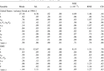
Having set the hyperparameters, we obtain draws from the joint posterior distribution of gap and model parameters follow-ing the Markov chain Monte Carlo (MCMC) scheme previously detailed. The chain runs 200,000 times after a burn-in phase of 100,000 iterations. Simulations are recorded every 10 itera-tions so all statistics reported are computed on samples of size 10,000. For a selection of variables of interest, Table 1 reports the sample mode and standard deviation, the autocorrelations at lags 1 and 5, the numerical standard error (NSE) associated with the sample mean, the relative numerical efficiency (RNE), and the pvalues of the Geweke (1992) convergence diagnos-tic (CD). The NSE is computed with a window on autocorre-lations of length 400. The RNE is obtained as the ratio of the NSE evaluated using only the output variance to the one that takes into account the sample autocorrelations. Geweke’s CD checks whether the average of the first 20% of simulations is significantly different from the average last 50%. The selection of variables we focus on is made up of the cycle periodicity and amplitude, the inverse signal-to-noise ratio Vc/Vp, the output mean growthμp, the contemporaneous correlation of the inno-vations in gap with those in inflationρcπ, the impact multipliers
βandλ, the scale parametersαm’s for the U.S. application, and the gap estimated at the last sample date.
The autocorrelations between draws are rather low because after only five lags the largest value is about .03 in absolute value. The NSE takes values of magnitude 10−1for the period-icity, 10−2for the cycle point estimates and the signal-to-noise ratio, and less than 10−2 for all other parameters. Hence, the number of draws seems sufficient to estimate the posterior dis-tribution and the moments of every quantity of interest with a fair accuracy. Because the RNE values are almost always above 50%, this precision is comparable to what we would have achieved with independent samples of half-size. Only for the U.S. second-period inverse signal-to-noise ratio does the RNE take the relatively low value of 40%. The Geweke tests are never rejected at the 5% level so chain convergence is obtained. We, thus, turn to analysis of the results.
Figure 1 displays prior and posterior distributions of period-icity and amplitude of GDP cycles in both the United States and the EMU. It can be seen that the periodicity posterior mode is about 7 years for the United States and about 9 years for the EMU. Positive skewness makes posterior means slightly larger. For both the United States and the EMU, the posterior mode is a bit larger than that of the prior. Maybe this reflects the rel-atively long expansion of the 1990s. There seems to be more precision around the periodicity of cycles in the United States than in the EMU, but this is mainly due to the difference be-tween priors: Using the EU prior for U.S. data yields analogous dispersion. Even if the posterior mode of the U.S. cycle peri-odicity is stable enough, the data appear to be only moderately informative for this parameter. More precision is obtained for the cycle amplitude parameter. With a mode of .8 and a com-parable dispersion, the posterior distributions of U.S. and EMU cycle amplitude seem much alike. This suggests that a similar number of quarters is necessary to both economies for absorb-ing a demand shock.
Table 1. MCMC efficiency and convergence diagnostics
Model specification
GDP: yt=pt+ct,pt=μp+apt,ct−2Acos{2π/τ}ct−1+A2ct−2=act Inflation: φπ(L)πt=μπ+βct−1+λyt−1+a∗πt
NSE
Variable Mode Sd. ρ1 ρ5 (×10−2) RNE CD
United States: variance break at 1984-1
τ 27.18 8.36 .02 .00 4.89 1.46 .44
A .82 .05 .20 .01 .06 .46 .74
μp .76 .04 .00 .00 .03 1.07 .23 αcVc/αpVp .32 .42 .37 .03 .50 .36 .98 ρcπ .14 .09 .02 .00 .06 1.07 .45
λ .04 .03 .01 .00 .02 1.45 .53 β .04 .02 .06 .00 .02 .81 .54 αp .18 .08 .06 .00 .07 .73 .36 αc .15 .09 .07 .01 .06 .96 .47 απ .53 .12 .01 .00 .09 .80 .98
c2005-3 .50 .86 .00 .01 .71 .74 .68
EMU
τ 35.21 12.67 .00 .00 8.15 1.21 .79
A .83 .05 .10 .00 .04 .99 .58
μp .59 .04 .00 .00 .03 .63 .40
Vc/Vp .33 .19 .21 .01 .16 .73 .84
ρcπ .26 .12 .03 .00 .09 .93 .45
λ .08 .04 .00 .00 .02 1.23 .62 β .04 .02 .05 .01 .01 1.16 .07
c2005-3 −.44 1.11 .01 .00 .69 1.27 .63
NOTE: ρcπ is the correlation betweenactandaπt; Sd. stands for standard deviation;ρjrepresents the lag-jautocorrelation; NSE is the
numerical standard error of the mean; RNE is relative numerical efficiency; and CD denotes thepvalue of the Geweke convergence statistic.
Figure 1. Densities of cycle periodicity and amplitude (- - prior; — posterior).
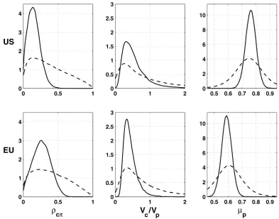
Figure 2. Densities of correlation between innovations in gap and in inflation, of inverse signal-to-noise ratio, and of output mean growth rate (- - prior; — posterior).
Figure 2 shows the prior and posterior distributions of the correlation coefficientρcπ, the inverse signal-to-noise
ra-tioVc/Vp, and the output mean growth rateμp. For the United States, the inverse signal-to-noise ratio reported is that obtained in the second sample period, that is,αcVc/(αpVp). As can be seen, besides imposing a positive correlation, our priors are diffuse enough. The posterior distribution ofρcπis highly
con-centrated around a mode of about .15 for the United States and about .25 for the EMU. For both the United States and the EMU, the variance of the shocks in the gap is roughly one third of the variance of the long-term shocks, and this is obtained with a good accuracy: Shocks on potential output are, thus, dominating these two GDP series. Notice that the posterior dis-tributions put no weight on Vc =0 and Vp=0. Hence, the pile-up problem mentioned in the Introduction does not occur.
Figure 2 also shows the distribution of the output mean growth rate: the posterior modes imply an average annual growth rate of about 3.0% for the United States and 2.4% for the EMU.
Figure 3 displays the prior and posterior densities of the scale parametersα’s. The standard deviations of both trend and cycle innovations are reduced by slightly more than one half, mak-ing the signal-to-noise ratio almost constant. The moderation of the inflation shocks is less pronounced, of order one third. The remarkable posterior precision around the scale parameters confirms the relevance of the variance break specification for U.S. GDP and inflation.
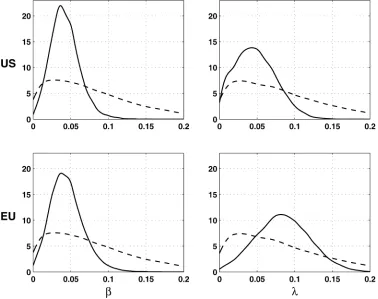
Figure 4 presents the prior and posterior distributions of the impact multipliersβ andλ. The posterior distributions put small weight in the neighborhood of 0 so the data seem to vali-date the prior restriction on positive responses. More constancy
Figure 3. Densities of scale factors (- - prior; — posterior).
Figure 4. Densities of impact multipliers (- - prior; — posterior).
can be seen in the posterior response of inflation to shocks on the gap than to shocks on the output growth. Because the gap and output growth mainly differ in the periodicity of their movements, it may be the noise amplification that the differ-encing operation implies that has obscured the empirical link with inflation. This result suggests that Phillips curve regres-sions can be sensitive to the dynamic properties of the proxy used for describing detrended output, as also discussed in Gali et al. (2001).
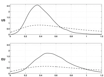
Figure 5 shows the dynamic response of inflation to a shock on the gap with associated 90% highest posterior density re-gion (HPD; see Box and Tiao 1973, chap. 2.8). This im-pulse response function is obtained as the posterior mean of the polynomial{β+λ(1−L)+κπφc(L)}/{φc(L)φπ(L)}. The
total inflationary effect of a shock on the gap is then {β + κπφc(1)}/{φc(1)φπ(1)}; its posterior distribution is displayed
in Figure 6, together with the distribution implied by the para-meter priors. It can be seen that, besides positiveness, we have not constrained the shape of the response by very much. The dynamics of the propagation of a shock on the gap is similar in the United States and in the EMU: After the 1 year, the infla-tionary effects are not significantly different from 0 at the 10% level. Besides the contemporaneous reaction related to the cor-relation parameter, the largest impact on inflation of a shock on the gap occurs with a three-quarter delay. The total response of inflation is slightly stronger in the euro area than in the United States. According to posterior modes, a 1-percentage-point rise in the gap in one quarter yields an inflation pressure of about .45 points for the EMU against .38 for the United States. There is, however, more uncertainty for the EMU than for the United States.
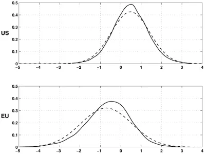
Figure 7 shows the posterior mean of the gap all along the sample together with the maximum likelihood (ML) estimates. For both the United States and EMU, the Bayesian and the ML estimates are very close to each other. The sequence of turning points suggests a delay in the fluctuations of the EMU economy with respect to the United States. For instance, the four highest peaks in the U.S. data occur in 1973-2, 1978-4, 1989-2, and 2000-2 and are followed by peaks in the EMU data in 1974-1, 1980-1, 1990-4, and 2000-3. Figure 7 also displays the 90% HPD interval and the 90% ML confidence bands computed with the Ansley–Kohn (1986) procedure that accounts for parame-ter uncertainty. Both inparame-tervals are cenparame-tered around the null hy-pothesis of a zero-gap estimate. The effect of the U.S. variance break is quite evident: The confidence interval shrinks by one half in the second period. With respect to the constant parameter model, the variance change yields a noticeable reduction of un-certainty after the break. For the EMU and the United States in the last period, ML and Bayesian analysis yield a similar accu-racy, with a slight advantage to the Bayesian approach. Figure 8 shows the posterior distribution of the gap estimate for the third quarter of 2005, the last point of the sample, together with the asymptotic distribution of the ML gap estimate. It can be seen that for both the EMU and the United States, the use of prior in-formation implies a nonnegligible gain in accuracy, even though our priors were not very restrictive. This illustrates the useful-ness of the Bayesian framework for characterizing unobserved patterns when evidence in the data is only moderate.
5. MODEL EXTENSIONS
Model (2.1)–(2.5) can also be used for estimating long-term unemployment or NAIRU. In this case, the trend equation
Figure 5. Average response of change in inflation to a shock on output gap with 90% HPD region.
in (2.1) needs to be modified as unemployment series are typi-cally better described as a second-order random walk than as a random walk plus drift. The trend equation, thus, becomes
pt=μpt−1+apt,
(5.1) μpt=aμt,
whereaμtis a Gaussian white noise with varianceVμthat is
or-thogonal to all other innovations. Because the stationary
trans-Figure 6. Posterior density of total response of change in inflation to a shock on output gap (- - prior; — posterior).
Figure 7. Gap posterior mean (—) with 90% HPD region ML estimate (- - -) with 90% confidence bands.
formation ofytis now2yt, the output growth regressor in the Phillips curve equation (2.2) or (2.3) must be replaced by2yt. The cycle equation (2.4) is left unchanged. The state space
rep-resentation in Section 3.1 must be modified, the state becoming ξt=(pt, μt,ct,ct−1, κπact+aπt)′with associated noise vector
wt=(apt,aμt,act,0, κπact+aπt)′. For the prior on the trend
Figure 8. Densities of output gap in 2005-3 Bayesian (—) versus ML (- - -).
parameters, we consider
p(Vp)=IG(sp0,vp0),
p(Vμ)=IG(sμ0,vμ0).
The full conditional of interest isp(Vp,Vμ|pT, μTp). The likeli-hood factorizationp(pT, μTp|Vp,Vμ)=p(pT|μTp,Vp)p(μTp|Vμ)
and the prior independence assumption allow us to consider
p(Vp|pT, μTp)andp(Vμ|μTp)sequentially. Specifying inverted Gamma prior distributions forVpandVμyields full
condition-als such that
Letting the prior of all the other parameters remain unchanged makes the analysis in Section 3 still valid. One column of ma-trixZin (3.1) needs to be modified, however, as it must embody 2yt instead of yt. This also implies that the Yule–Walker procedure in Appendix B must be corrected. Samples of the state in its first time period can be obtained using the results in Appendix A. Notice that two elements of the state now need to be sampled,ct−1andμt.
As in Section 3.3, a break in the variancesVp andVμ at a
specified datetBcan be introduced. Letαμdenote the
parame-ter indexing the slope variance reduction. Still assuming inde-pendent Beta priors Beta(aαm,bαm)form=p, μ, samples from
p(Vp|αp,pTμTp)andp(Vμ|αμ, μTp)can be obtained as before af-ter a simple rescaling of the second-period shocksaTpt
Banda
Sometimes model (2.1)–(2.5) or its NAIRU version arises as the reduced form of a macroeconomic model; see, for exam-ple, Planas et al. (2007). In this case, it is likely that the struc-tural model suggests that some economic variables should also explain the inflation dynamics. Thanks to the flexibility of the NIG framework, such exogenous regressors can be added with-out difficulty using the results of Section 3.
Finally, it is worth considering the possibility of a correlation of shocks on the cycle with those on the trend level. A uni-variate decomposition of U.S. GDP with correlated compo-nents has recently been discussed in Morley, Nelson, and Zivot (2003). Whether the long-term trend and the short-term fluc-tuations in GDP should be correlated is an open issue: As far as we know, no compelling reason for such a correlation has yet been produced. Harvey and Koopman (2000) pointed out, however, several shortcomings of such decompositions. Never-theless, interested readers can easily introduce this correlation into model (2.1)–(2.4). The simplest way is to specify the cycle equation (2.4) as in
1−2Acos(2π/τ )L+A2L2ct=a∗ct
and to represent the short-term innovationsa∗ctasa∗ct≡κcapt+
act,κc being a real parameter. The correlation with long-term
shocks is then trivially obtained asρcp=κcVp/
κ2
cVp+Vc. This parameterization is similar to the one used in (2.3); it has the advantage thatapt,act, andaπt are uncorrelated. The prior for(κc,Vc)becomes
p(κc,Vc)=NIG(κc0,Mc−01,sc0,vc0).
The full conditional of interest is nowp(κc,Vc|A, τ,cT,Vp,aTp), the other ones being unchanged. We have
p(κc,Vc|A, τ,cT,Vp,aTp)
As before, the Normal-inverse Gamma framework leads to
T κcapt+act,aptbeing handled as a weakly exogenous regressor. The innovationapt is obtained as eitherapt=pt−pt−1−μp orapt=pt−pt−1−μpt−1according to the model specification
considered. When samplingκcandVc, the conditioning on the cycle starting values can be removed using this NIG distribu-tion as proposal in a Metropolis–Hastings step. The acceptance probability of the candidate(κc,˜ V˜c)is
Because a similar step is used when sampling δ andVπ,
al-together the first two moments of(π1, π2,c1,c2), givenVc,
κc,A,τ,aTp,δ, andVπ, will be needed. They can be obtained
us-ing the Yule–Walker procedure detailed in Appendix B, slightly modified to take into account the correlation between long-term and short-term shocks. A further difficulty arises when consid-ering the trend model (5.1) becauseμp0 is never sampled, so ap1 is not available andaTp reduces to aTp2. A simple solution
is to compute the second moments of(π1, π2,c1,c2,ap2),
givenVc,Vp,κc,A, andτ, and then to condition onap2.
We experienced this extension on U.S. and EMU GDP and inflation data using a flat prior on κc. The posterior means of the gap were very close to those obtained under the orthogo-nality assumption, with similar 90% highest posterior region. We do not investigate further the possibility of cross-correlated components mainly because we believe that a compelling moti-vation is still needed. Besides, the statistical properties of such decompositions deserve further exploration, maybe in a later research.
6. CONCLUSION
In this article we have developed a Bayesian analysis of Kut-tner’s bivariate Phillips curve model for estimating output gaps. The analysis involves a Gibbs sampling scheme where use is made of a particular likelihood factorization and of a prior in-dependence assumption in order to sample parameters given the state in three blocks. The conditioning on the first inflation ob-servations is removed with a Metropolis–Hastings step. We also reparameterized the cyclical AR(2) specification in terms of the polar coordinates of the characteristic equation roots, mainly because noninformative priors on AR parameters put too much emphasis on short-term periodicities and persistent movements. Besides being quite natural for describing cycles, the flexibil-ity of the polar coordinate parameterization was important to get interpretable results. We resorted to the adaptive rejection Metropolis method for sampling periodicity and amplitude pa-rameters. We also discussed several model extensions, includ-ing variance moderation. This methodology enables potential output and NAIRU estimates to incorporate prior information. Given the amount of macroeconomic knowledge and business cycle studies available, we believe that this Bayesian frame-work will appeal to practitioners. We have made it available in Program GAP, Version 4.0, which can be downloaded at
www.jrc.cec.eu.int/uasa/prj-gap.asp.
We applied this methodology to the analysis of output gap in the EMU and U.S. economies. The results show that the data agree with Phillips curve theory. For both the EMU and the United States, we could observe a sharp response of inflation to the gap and a more volatile reaction to output growth. Hence, care should be taken when choosing a detrended GDP proxy for fitting the Phillips curve. We also obtained response functions of EMU and US inflation to shocks to the gap with a similar dy-namic. EMU inflation, however, seems slightly more reactive to shocks on the gap. The posterior distribution of the cycle peri-odicity never appears very precise, a point that would deserve a focused investigation. Given our priors, the gap posterior mean was found to be in close agreement with the ML estimates. Yet the gain in accuracy achieved with the Bayesian approach was
noticeable, showing that prior information can help in charac-terizing unobserved patterns when evidence in the data is only moderate.
ACKNOWLEDGMENTS
The views expressed here are those of the authors and do not necessarily reflect the official position of the European Com-mission. Gabriele Fiorentini acknowledges financial support from MIUR. We are grateful to Juanjo Dolado, Gabriel Perez-Quiros, Werner Roeger, Herman Van Dijk, an associate editor, and two anonymous referees for their useful comments. Com-putations can be replicated using a software developed by the authors and available atwww.jrc.cec.eu.int/uasa/prj-gap.asp.
APPENDIX A: DERIVATION OFξ1|1 ANDP1|1
The initial state vector can generally be written as
ξ1=a+Aδ+Bη, η∼N(0,I), δ∼N(0,kI),
wherek→ ∞,ais a vector of constants, andAandBare known matrices. This formulation implies
ξ1∼N(a,P),
whereP=P⋆+kP∞,P⋆=BB′, andP∞=AA′. Nonzero
ele-ments in the matrixP∞ correspond to the diffuse elements of the state. Letd denote the number of nonstationary elements of the state. The algorithm proposed by de Jong (1991) yields ξd+1|d andPd+1|d. Koopman (1997) further extended it to get
ξ1|1,P1|1, . . . , ξd|d,Pd|d. We implemented Koopman’s
algo-rithm as follows.
Conditional on the first observation, the first two moments of the state at timet=1 are q<N. Following lemma 2 in Koopman (1997), we obtain the
N×NmatrixQ= [Q1(N×q)Q2(N×(N−q))]that partially
and similarly forS∞,1, it can be seen that the solutions are
whereV2and2are the matrices of eigenvectors and
eigenval-ues ofS⋆22. The matrixQ1is instead obtained as
whereV1and1are the matrices of eigenvectors and
eigenval-ues ofS∞,1. Then, according to theorem 2 in Koopman (1997),
For convenience, we focus on the joint moments of(π1,
π2,c1,c2). Trivially, E(c1) =E(c2) = 0 and E(π1) = Using both equations (2.1) and (2.2), we have
γπ y,1=φπ1γπ y,0+φπ2γπ y,−1
Proceeding similarly for the cross-moments betweenπt andct yields
The system (B.1)–(B.3) is then solved with the termsγck,k=
0,1,2, directly obtained from (2.1) or (2.4).
[Received February 2004. Revised May 2006.]
REFERENCES
Ansley, C. F., and Kohn, R. (1986), “Prediction Mean Squared Error for State Space Models With Estimated Parameters,”Biometrika, 73, 467–473. Apel, M., and Jansson, P. (1999a), “A Theory-Consistent Approach for
Esti-mating Potential Output and the NAIRU,”Economics Letters, 64, 271–275. (1999b), “System Estimate of Potential Output and the NAIRU,” Em-pirical Economics, 24, 373–388.
Barnett, G., Kohn, R., and Sheater, S. (1996), “Bayesian Estimation of Autore-gressive Model Using Markov Chain Monte Carlo,”Journal of Economet-rics, 74, 237–254.
Bauwens, L., Lubrano, M., and Richard, J. (1999),Bayesian Inference in Dy-namic Econometric Models, Oxford, U.K.: Oxford University Press. Billio, M., Monfort, A., and Robert, C. (1999), “Bayesian Estimation of
Switch-ing ARMA Models,”Journal of Econometrics, 93, 229–255.
Blanchard, O., and Simon, J. (2001), “The Long and Large Decline in US Out-put Volatility,”Brookings Papers on Economic Activity, 2001:1, 135–164. Box, G., and Tiao, G. (1973),Bayesian Inference in Statistical Analysis,
Read-ing, MA: Addison-Wesley.
Carter, C., and Kohn, R. (1994), “On Gibbs Sampling for State Space Models,”
Biometrika, 81, 541–553.
Casella, G., and George, E. (1992), “Explaining the Gibbs Sampler,”The Amer-ican Statistician, 46, 167–173.
Chib, S. (1993), “Bayesian Regression With Autoregressive Errors: A Gibbs Sampling Approach,”Journal of Econometrics, 58, 275–294.
Chib, S., and Greenberg, E. (1994), “Bayesian Inference in Regression Models With ARMA(p,q) Errors,”Journal of Econometrics, 64, 183–206.
(1995), “Understanding the Metropolis–Hastings Algorithm,” The American Statistician, 49, 327–335.
Clark, P. (1987), “The Cyclical Comovement of U.S. Economic Activity,”
Quarterly Journal of Economics, 102, 797–814.
de Jong, P. (1991), “The Diffuse Kalman Filter,”The Annals of Statistics, 2, 1073–1083.
de Jong, P., and Shephard, N. (1995), “The Simulation Smoother for Time Se-ries Models,”Biometrika, 82, 339–350.
Durbin, J., and Koopman, S. (2001),Time Series Analysis by State Space Meth-ods, Oxford, U.K.: Oxford University Press.
(2002), “A Simple and Efficient Simulation Smoother for State Space Time Series Analysis,”Biometrika, 89, 603–616.
Fagan, G., Henry, J., and Mestre, R. (2001), “An Area-Wide Model for the Euro Area,” Working Paper 42, European Central Bank.
Gali, J., Gertler, M., and Lopez-Salido, D. (2001), “European Inflation Dynam-ics,”European Economic Review, 45, 1237–1270.
Gerlach, S., and Smets, F. (1999), “Output Gap and Monetary Policy in the EMU Area,”European Economic Review, 43, 801–812.
Geweke, J. (1992), “Evaluating the Accuracy of Sampling-Based Approaches to the Calculation of Posterior Moments,” inBayesian Statistics, Vol. 4, eds. J. Bernardo, J. Berger, A. Dawid, and A. Smith, Oxford, U.K.: Oxford Uni-versity Press, pp. 169–194.
(1999), “Using Simulation Methods for Bayesian Econometric Mod-els: Inference, Development, and Communication,”Econometric Reviews, 18, 1–73.
Gilks, W., Best, N., and Tan, K., (1995), “Adaptive Rejection Metropolis Sam-pling With Gibbs SamSam-pling,”Applied Statistics, 44, 455–472.
Gilks, W., Neal, R., Best, N., and Tan, K., (1997), “Corrigendum: Adaptive Rejection Metropolis Sampling,”Applied Statistics, 46, 541–542.
Gómez, V., and Maravall, A. (1996), “Programs Seats and Tramo: Instructions for the User,” Working Paper 9628, Bank of Spain.
Hall, R., and Taylor, J. (1991),Macroeconomics, New York: Norton. Harvey, A. (1981), Time Series Models(2nd ed.), Hertfordshire: Harvester
Wheatsheaf.
Harvey, A., and Koopman, S. (2000), “Signal Extraction and the Formulation of Unobserved Components Models,”Econometrics Journal, 3, 84–107. Harvey, A., Trimbur, T., and van Dijk, H. (2002), “Cyclical Components in
Eco-nomic Time Series: A Bayesian Approach,” Cambridge, U.K.: Cambridge University Press.
Kichian, M. (1999), “Measuring Potential Output With a State-Space Frame-work,” Working Paper 99-9, Bank of Canada.
Kim, C.-J., and Nelson, C. R. (1999), “Has the US Economy Become More Stable? A Bayesian Approach Based on a Markov-Switching Model of the Business Cycle,”Review of Economics and Statistics, 81, 608–616. Koop, G., and van Dijk, H. (2000), “Testing for Integration Using Evolving
Trend and Seasonal Models: A Bayesian Approach,”Journal of Economet-rics, 97, 261–291.
Koopman, S. (1997), “Exact Initial Kalman Filtering and Smoothing for Non-stationary Time Series Model,”Journal of the American Statistical Associa-tion, 92, 1630–1638.
Kuttner, K. (1994), “Estimating Potential Output as a Latent Variable,”Journal of Business & Economic Statistics, 12, 361–368.
McConnell, M. M., and Perez-Quiros, G. (2000), “Output Fluctuations in the United States: What Has Changed Since the Early 1980’s,”American Eco-nomic Review, 90, 1464–1476.
McCulloch, R., and Tsay, R. (1994), “Bayesian Analysis of Autoregressive Time Series via the Gibbs Sampler,”Journal of Time Series Analysis, 15, 235–250.
Morley, J., Nelson, C., and Zivot, E. (2003), “Why Are the Beveridge–Nelson and Unobserved Components Decompositions of GDP so Different?”Review of Economics and Statistics, 85, 235–243.
Organization of Economic Cooperation Development (2000), “The Concept, Policy Use and Measurement of Structural Unemployment,” Annex 2 of “Es-timating Time-Varying NAIRU’s Across 21 OECD Countries,” Paris: Author. Orphanides, A., and van Norden, S. (2002), “The Unreliability of Output Gap Estimates in Real-Time,”Review of Economics and Statistics, 84, 569–583. Planas, C., Roeger, W., and Rossi, A. (2007), “How Much Has Labour Taxation
Contributed to European Structural Unemployment?”Journal of Economic Dynamics & Control, to appear.
Stock, J., and Watson, M. (1998), “Median Unbiased Estimation of Coefficient Variance in a Time-Varying Parameter Model,”Journal of the American Sta-tistical Association, 93, 349–358.
(2002), “Has the Business Cycle Changed and Why?” Working Paper 9127, National Bureau of Economic Research.
Taylor, J. (1993), “Discretion versus Policy Rules in Practice,”Carnegie– Rochester Conference Series on Public Policy, 39, 195–214.
Tierney, L. (1994), “Markov Chains for Exploring Posterior Distributions,”The Annals of Statistics, 22, 1701–1762.
Watson, M. (1986), “Univariate Detrending Methods With Stochastic Trends,”
Journal of Monetary Economics, 18, 49–75.
Zellner, A. (1996),An Introduction to Bayesian Inference in Econometrics
(2nd ed.), New York: Wiley.