Full Terms & Conditions of access and use can be found at
http://www.tandfonline.com/action/journalInformation?journalCode=ubes20
Download by: [Universitas Maritim Raja Ali Haji] Date: 12 January 2016, At: 17:57
Journal of Business & Economic Statistics
ISSN: 0735-0015 (Print) 1537-2707 (Online) Journal homepage: http://www.tandfonline.com/loi/ubes20
Mimicking Portfolios, Economic Risk Premia, and
Tests of Multi-Beta Models
Pierluigi Balduzzi & Cesare Robotti
To cite this article: Pierluigi Balduzzi & Cesare Robotti (2008) Mimicking Portfolios, Economic Risk Premia, and Tests of Multi-Beta Models, Journal of Business & Economic Statistics, 26:3, 354-368, DOI: 10.1198/073500108000000042
To link to this article: http://dx.doi.org/10.1198/073500108000000042
View supplementary material
Published online: 01 Jan 2012.
Submit your article to this journal
Article views: 153
Mimicking Portfolios, Economic Risk Premia,
and Tests of Multi-Beta Models
Pierluigi B
ALDUZZIBoston College, Finance Department, The Wallace E. Carroll School of Management, Chestnut Hill, MA 02467 (balduzzp@bc.edu)
Cesare R
OBOTTIFederal Reserve Bank of Atlanta, Research Department, 1000 Peachtree Street NE, Atlanta, GA 30309 (cesare.robotti@atl.frb.org)
We consider two formulations of the linear factor model (LFM) with nontraded factors. In the first formu-lation, LFM, risk premia and alphas are estimated by a cross-sectional regression of average returns on betas. In the second formulation, LFM⋆, the factors are replaced by their projections on the span of excess returns, and risk premia and alphas are estimated by time series regressions. We compare the two formu-lations and study the small-sample properties of estimates and test statistics. We conclude that the LFM⋆ formulation should be considered in addition to, or even instead of, the more traditional LFM formulation.
KEY WORDS: Mimicking portfolios; Economic risk premia; Linear factor models.
1. INTRODUCTION
Most asset-pricing models explain the cross-section of ex-pected returns in terms of exposures, or betas, to one or more risk factors. We call these models multi-beta models. In the consumption-based capital asset pricing model (C–CAPM) and the intertemporal capital asset pricing model (I–CAPM), one or more of the risk factors are “economic” and they are not them-selves asset returns. The standard formulation of such asset-pricing models starts from a linear factor model (LFM),
rt=α+β⊤[λ+yt−E(yt)] +et, (1) wherert is an N×1 vector of returns in excess of the risk-free rate,αis the vector of deviations from the model,λis the vector of economic risk premia,yt is aK×1 vector of factor realizations, andetis anN×1 vector of residuals orthogonal to the factors. If the multi-beta model is correct, thenα=0, and a unit-beta portfolio (i.e., any portfolio with a beta of 1 with respect to factorykand 0 with respect to all the other factors) earns a risk premium equal toλk.
The risk premia on the unit-beta portfolios can be immedi-ately estimated as the coefficients (or averages of coefficients) of a cross-sectional regression (CSR) of average returns (or re-turns) on the betas. This CSR can be performed using various weighting schemes. Here we focus on two of these schemes. In the first scheme, the assets are unweighted. This corresponds to a CSR ordinary least squares (OLS) style, following the semi-nal articles of Black, Jensen, and Scholes (1972) and Fama and MacBeth (1973). This approach has been implemented in nu-merous empirical studies. In the second scheme, the assets are weighted by the inverse of the covariance matrix of the idiosyn-cratic components. This corresponds to a CSR generalized least squares (GLS) style.
An alternative formulation of the LFM is obtained when we replace the factors with the variable component of their pro-jections onto the span of the excess returns, augmented with a constant (see Huberman, Kandel, and Stambaugh 1987). We have
yt=γ0⋆+(γ
⋆)⊤r
t+ǫt (2)
and y⋆t ≡(γ⋆)⊤rt, where γ⋆ =rr−1ry. For the mimicking portfolios,y⋆t, to exist we assume that(γ⋆)⊤1N=yrrr−11N= 0K, where 1Nis anN×1 vector of 1’s and 0Kis aK×1 vector of 0’s. This condition is equivalent to assuming that the global minimum-variance portfolio has positive systematic risk. We then have
rt=α⋆+(β⋆)⊤y⋆t +e⋆t. (3) We denote this alternative formulation as LFM⋆.
The projection coefficients are the weights of portfolios whose returns have maximum (squared) correlations with the factors. Thus, these maximum-correlation portfolio weights are proportional to the hedging-portfolio weights of Merton (1973). Other examples of this second approach have been pro-vided by Breeden (1979), Breeden, Gibbons, and Litzenberger (1989), Fama (1996), Lamont (2001), and Ferson, Siegel, and Xu (2005).
Table 1 presents results for the LFM and the LFM⋆ formu-lations of the C–CAPM. (Details on the estimation procedures and the data used are given later in the article.) Table 1 shows how, depending on the linear factor model, parameter estimates and statistical inferences can differ substantially: The consump-tion risk premium is .24 and significant in the LFM (CSR–OLS) but only .01 and insignificant in the LFM⋆. Moreover, the test
of overidentifying restrictions leads to a strong rejection of the C–CAPM in the LFM⋆ formulation but only to a weak rejec-tion in the CSR–OLS version of the LFM formularejec-tion. The lit-erature does not explain the theoretical relation between these two sets of results, nor does it establish which representation is most likely to deliver the correct estimates and inference.
One contribution of this article is to clarify the relationships between the LFM and LFM⋆ formulations and between unit-beta and maximum-correlation portfolios. We show thatα=0 if and only if α⋆=0, that λ=λ⋆ ifα=0 and if the factors are traded (yt=y⋆t), and that the estimates ofαandα⋆coincide
© 2008 American Statistical Association Journal of Business & Economic Statistics July 2008, Vol. 26, No. 3 DOI 10.1198/073500108000000042
354
Table 1. LFM versus LFM⋆representations
LFM C–CAPM LFM⋆C–CAPM
λOLS λGLS χOLS2 χGLS2 λ∗ χ2 Estimate .24 .09 17.94 23.92 .01 28.66
t-ratio 2.23 1.43 1.03
p-value .026 .152 .036 .004 .300 .001
NOTE: Here we estimate a C–CAPM economy. Parameter estimates of the LFM are ob-tained by cross-sectional regression, withW=I(OLS) andW= ˆee−1(GLS). Estimates of
the parameters of the LFM⋆are obtained by time series regressions. Asymptotic standard errors and chi-squared statistics are obtained by GMM, assuming no serial dependence. The sample is from 1959:03–2002:11. We consider the 10 size portfolios as the test assets.
when the CSR is GLS style. We also show that when the unit-beta mimicking portfolios have minimum idiosyncratic risk, we can obtain the same Sharpe ratio from maximum-correlation portfolios and from unit-beta mimicking portfolios. Finally, we show how the construction of “mimicking portfolios” allows us to translate characteristic-based explanations of the cross-section of stock returns into risk-based explanations.
Following Hansen (1982) and Cochrane (2001), we show how both formulations of the linear factor model, and both es-timation approaches (CSR and time series), can be cast within the unifying framework of the generalized method of moments (GMM). This approach allows us to derive the asymptotic prop-erties of estimates and statistics without the need for restrictive distributional assumptions. We then construct a simulation ex-ercise to assess the properties of the estimators for the two dif-ferent formulations of the model. The simulations consider a one-factor (C–CAPM) and a two-factor (I–CAPM) economy, both iid and serially correlated data, different lengths of the sample (525 vs. 240 months), and different choices of test as-sets (10 size-sorted portfolios vs. the 25 size- and value-sorted portfolios of Fama and French 1993).
Summarizing our simulation exercises, the LFM⋆
formula-tion performs better than the LFM–CSR–GLS formulaformula-tion and similar to the LFM–CSR–OLS formulation in terms of bias of the risk premium estimates. In terms of root mean squared er-rors (RMSEs) of the risk premium estimates and power of the tests, the LFM⋆ and LFM–CSR–GLS perform similarly and better than the LFM–CSR–OLS formulation. In the case of a noisy factor, the LFM⋆formulation works much better than ei-ther LFM formulation. Our small-sample analysis should help researchers draw the correct conclusions when facing different results from different methods. For example, an econometri-cian faced with the results of Table 1 should be more (less) inclined to trust the risk premium estimates (test statistics) re-sulting from the LFM⋆representation than from the LFM
rep-resentation.
We also explore several extensions of the basic analysis sum-marized earlier. First, we consider the case of time-varying conditional moments and conditional versions of the LFM and LFM⋆formulations. In the presence of time-varying betas and risk premia, the LFM⋆ formulation performs worse than the LFM formulation in terms of bias but better in terms of RMSE of the risk premium estimates. Second, we consider the ap-proach of Lehmann and Modest (1988) to the construction of mimicking portfolios. Their approach generally does worse than the LFM⋆ formulation, in terms of both bias and RMSE
of the risk premium estimates. Third, we consider the correc-tion for small-sample bias in the CSR risk premium estimates, suggested by Chen and Kan (2006). In several cases, the bias adjustment actually leads to worse bias, and the bias-adjusted CSR estimators always have higher RMSEs than the nonad-justedλ⋆estimates. Fourth, we study the various methods in the case of long-horizon overlapping returns. Using long-horizon returns generally leads to higher biases and RMSEs, although in the case of the C–CAPM, these effects are more pronounced for the CSR risk premium estimates than for theλ⋆estimates. Finally, we consider the implications of the restrictions from the LFM and LFM⋆ formulations on covariance matrices, for the purpose of constructing minimum-variance portfolios. In-terestingly, the restrictions from the LFM⋆ formulation gener-ally lead to portfolios with better properties than the portfolios restricted using the LFM formulation.
For the aforementioned reasons, we conclude that the LFM⋆ formulation should be considered in addition to, or even instead of, the more traditional LFM formulation. This conclusion ap-plies not only to the estimation and testing of multi-beta mod-els, but also to the construction of mean–variance efficient port-folios.
The article is organized as follows. Section 2 provides a re-view of the literature. Section 3 presents the theoretical results. Section 4 derives the moment conditions used in estimation, and Section 5 derives the asymptotic properties of the GMM estimators. Section 6 discusses the case in which both traded and nontraded factors are present and the nontraded factor is observed with noise. Section 7 illustrates the data used to cali-brate the simulation exercise. Section 8 describes the bootstrap experiment, Section 9 discusses the results of the simulation, and Section 10 explores some extensions of the analysis. The final section summarizes our findings, and the Appendix con-tains proofs of the analytical results.
2. RELATED LITERATURE
Several authors have studied the properties of CSR risk premium estimators, including Litzenberger and Ramaswamy (1979), Amsler and Schmidt (1985), MacKinlay (1987), Shanken (1992), Shanken and Zhou (2007), Affleck-Graves and Bradfield (1993), Kim (1995), and Chen and Kan (2006). Others have focused on the comparison between stochastic dis-count factor (SDF) and LFM representations in tests of multi-beta models (see, e.g., Cochrane 2001; Kan and Zhou 1999, 2001a; Jagannathan and Wang 2002).
The theoretical properties of different mimicking portfolios and formulations of the LFM have been discussed by Grinblatt and Titman (1987), Huberman et al. (1987), and Kandel and Stambaugh (1995). Grinblatt and Titman showed that if the ar-bitrage pricing theory holds, then the portfolios of maximum likelihood factor analysis can be combined to obtain a Sharpe ratio as high as the maximum Sharpe ratio attainable from all of the available assets. Huberman et al. showed how unit-beta portfolios and maximum-correlation portfolios can replace the nontraded factors in linear factor models. Kandel and Stam-baugh showed how the CSR–GLS results, but not the CSR– OLS results, are invariant to the repackaging of the individual securities.
Our analysis focuses on risk exposures (i.e., betas) as the drivers of the cross-section of returns. Starting with Fama and French (1992), several authors have focused instead on “charac-teristics,” such as a company’s market capitalization and book-to-market ratio. Fama and French (1992) interpreted the char-acteristics as new indicators of risk exposure, and then later (1993) constructed long–short characteristic-sorted portfolios, showing that the exposures to the returns on those portfolios [Fama and French (FF) “factors”] explain the cross-section of average returns. The articles by Daniel and Titman (1997) and Brennan, Chordia, and Subrahmanyam (1998) challenged Fama and French’s risk-based interpretation, and Ferson (1996) and Ferson, Sarkissian, and Simin (1999) questioned the very pos-sibility of distinguishing between characteristic- and risk-based explanations.
The present article focuses on the comparison between two alternative formulations of a multi-beta model with nontraded factors. To the best of our knowledge, the only other author who has focused on this comparison is Kimmel (2003), who derived the asymptotic properties of estimates of risk premia on CSR–GLS unit-beta portfolios and on maximum-correlation portfolios. Kimmel’s work differs from ours because he focused on asymptotics only, for the case of Gaussian iid returns, and did not address issues of size and power of the test statistics.
Also related to the present work are the work of Asgharian (2004) and Asgharian and Hansson (2005). Asgharian showed how testing a multi-beta model in its LFM or LFM⋆formulation can lead to different conclusions. In addition, he discussed the “portfolio” method of estimating factor realizations, in which assets with a high loading on a factor receive a positive weight, and assets with a low loading on a factor receive a negative weight (see, e.g., Chan, Karceski, and Lakonishok 1998; Fama and French 1993). Asgharian’s work differs from ours because he did not study the theoretical relation between the LFM and LFM⋆ representations and did not compare the small-sample properties of risk premium estimates and test statistics for the two formulations. Asgharian and Hansson considered the ef-fects of replacing the original factors in the LFM with the factor realizations estimated using the portfolio method and an equally weighted scheme. Their work differs from ours because they fo-cused on the implications of the portfolio method, rather than on the properties of the LFM and LFM⋆representations.
3. THEORETICAL RESULTS
3.1 LFM and LFM⋆
Result 1 establishes the relation between the two representa-tions.
Result 1. Mispricing in the LFM⋆ representation relates to mispricing in the LFM representation as follows:
α⋆= [I−(β⋆)⊤(γ⋆)⊤]α, (4) where[I−(β⋆)⊤(γ⋆)⊤]is of rankN−Kwith null space given byβ⊤δ,δbeing a generic real-valuedN×1 vector.
Thus, if α=0, then α⋆=0. On the other hand, if α⋆ =
0, then α is not necessarily 0, because the N×N matrix
[I−(β⋆)⊤(γ⋆)⊤]is of rankN−K. Yet the only case in which
α⋆=0 andα=0 is when α=β⊤δ, but this means that the multi-beta model holds, although with parametersλ+δ. Thus we conclude thatα⋆=0 is a necessary and sufficient condition forα=0.
Result 2 obtains the relation between risk premia in the two formulations.
Result 2. We have
λ⋆=(γ⋆)⊤α+y⋆y⋆yy−1λ, (5) whereλ⋆=(γ⋆)⊤E(rt).
Thus a sufficient condition for the risk premia in the two for-mulations to be the same is thatα=0 and that the factors are traded (in which casey⋆y⋆=yy).
3.2 Cross-Sectional Regressions, Mimicking Portfolios, and Sharpe Ratios
The standard approach of running CSRs of average excess returns on betas leads to the risk-premium coefficients
˜
λ=(βWβ⊤)−1βWE(rt). (6) The CSR coefficients minimize the quadratic form
[E(rt)−β⊤λ˜]⊤W[E(rt)−β⊤λ˜]. (7) Two common choices for the weighting matrixW areW =I andW=ee−1. The first choice corresponds to an OLS regres-sion; the second, to a GLS regression. Alternatively, we can chooseW=rr−1.
Interestingly, we obtain the same CSR coefficients forW= rr−1as forW=ee−1. The intuition for this result is straightfor-ward: Minimizing the total portfolio variance with a constraint on systematic risk is equivalent to minimizing the idiosyncratic portfolio variance with a constraint on systematic risk. This re-sult proves to be useful when we consider an alternative inter-pretation of the CSR coefficients. First, we recognize that the K×Nmatrix
˜
γ⊤=(βWβ⊤)−1βW (8) is a matrix ofKsets ofNportfolio weights. Each portfolio has unit beta with respect to the chosen factor and zero betas with respect to all other factors included in the LFM,
˜
γ⊤β⊤=(βWβ⊤)−1βWβ⊤=I. (9) On the other hand, it is straightforward to show how the CSR portfolio weights correspond to the solution of the minimiza-tion problem (see, e.g., Litzenberger and Ramaswamy 1979; Huberman et al. 1987)
min
γk
γk⊤W−1γk,
(10) s.t. βγk=sk,
whereγk is the N×1 vector of portfolio weights andsk is a vector with thekth element equal to 1 and 0’s elsewhere.
Thus, whenW=I, the CSR portfolio weights minimize the length of the vector of portfolio weights, subject to the unit-beta constraint. WhenW=rr−1, the CSR portfolio weights mini-mize the variance of the mimicking portfolio returns, subject to the unit-beta constraint. This second set of portfolio weights is
equal to the set of portfolio weights implicit in the CSR–GLS coefficients(β−ee1β⊤)−1βee−1E(rt).
Note that the maximum-correlation portfolios are propor-tional to the solution of the minimization ofγk⊤rrγk with re-spect toγk, subject to thesingleconstraint ykrγk=1. Thus both unit-beta CSR–GLS portfolios and maximum-correlation portfolios minimize the variance of the portfolio returns subject to constraints on covariances. The difference is that the unit-beta portfolios are subject to constraints on covariances with allof the other factors, whereas the maximum-correlation port-folios are subject only to a single constraint on the covariance with the factor being tracked.
One additional property of the unit-beta portfolio weights is that forW=−rr1 (orW =ee−1), and, in the case of a single factor, the weights are proportional to the maximum-correlation mimicking-portfolio weights; in fact,
˜
γ⊤=(β−rr1β⊤)−1βrr−1
(11)
=(yrrr−1ry/σy2)−1yrrr−1.
Because(yrrr−1ry/σy2)in the one-factor case is a scalar,γ˜⊤ here is proportional toyr−rr1=(γ⋆)⊤. In the general case of Kfactors, on the other hand, the unit-beta mimicking-portfolio weightsγ˜arelinear combinationsof the maximum-correlation mimicking-portfolio weightsγ⋆.
Note, however, that the foregoing discussion does not mean that in the presence of a single nontraded factor, the properties of the estimates of the risk premium on the CSR–GLS portfolio and on the maximum correlation portfolio are the same. In fact, although the maximum-correlation portfolios are constructed subject to a covariance constraint, the CSR–GLS portfolios are constructed subject to abetaconstraint. In general, covariance and beta estimates have different properties that lead to differ-ent properties of the risk premium estimates. For example, in the case of a noisy factor, covariance estimates are consistent, whereas beta estimates are not (more on this in Sec. 6.2). This leads to different behaviors of the two risk premium estimates, even when only one factor is at work.
Result 3 shows how the alphas associated with the CSR pre-mia equal the alphas of the LFM⋆ representation when W = ee−1(orW=rr−1).
Result 3. WhenW=ee−1, α⋆= ˜α.
Result 4 discusses the relation between Sharpe ratios attain-able from different mimicking portfolios.
Result 4. When W =−ee1, then the maximum squared Sharpe ratio from investment in the unit-beta mimicking portfo-lios equals the maximum squared Sharpe ratio from investment in the maximum-correlation portfolios.
This means that in the case of a single factor, the Sharpe ra-tios on the two types of mimicking portfolios are the same.
3.3 Mimicking Portfolios and Characteristic-Based Models
Our analysis focuses on multi-beta models, that is, risk-based models of expected returns. Yet the mimicking-portfolio ap-proach allows us to revisit the formulation of
characteristic-based models in terms of exposure to characteristic-sorted port-folios (e.g., Fama and French 1993). Indeed, Result 5 estab-lishes the “observational equivalence” between characteristic-based and risk-characteristic-based models; we can always formulate a characteristic-based model as a multi-beta model with traded factors.
Result 5. Assume that expected returns are linearly related to security characteristics
E(rt)=H⊤δ, (12) whereHis a full-rankK×Nmatrix of characteristics andδis aK×1 vector. We can always construct a set ofK minimum-variance, unit-characteristic portfolios with returns¯yt, such that
E(y¯t)=δ (13)
and
y−¯y¯1¯yr≡ ¯β=H. (14) One implication of Result 5 is that securities with the same characteristics also have the same exposures to unit-characteristic portfolio returns. This may explain why, after controlling for characteristics, average portfolio returns are not related to their exposures to the FF factors (Daniel and Titman 1997). Moreover, for Result 5 to hold, the unit-characteristic portfolios must have weights that are the coefficients of a GLS-style CSR of expected returns on characteristics. The FF fac-tors are not constructed in such a way, which may explain why, even after controlling for the exposure to the FF factors, the cross-section of average stock returns still exhibits significant characteristic-driven patterns (Brennan et al. 1998).
Note that the observational equivalence between characteris-tic- and risk-based explanations also is demonstrated in the the-oretical analyses of Ferson (1996) and Ferson et al. (1999). Ferson’s result differs from ours, because he assumed the or-thogonality between security characteristics and risk exposures, together with either a factor structure in returns or a time vari-ation in theδcoefficients; for a comparison, we need only as-sume thatrris invertible. Ferson et al.’s analysis also differs from ours, because they considered unit-characteristic portfo-lios constructed by means of anOLS-styleCSR and assumed a covariance matrix of returns proportional to the identity matrix.
4. MOMENT CONDITIONS
Here we illustrate the moment conditions imposed in esti-mating the two formulations of the linear factor model.
4.1 LFM
Letztdenote the data andθdenote the parameter vector. The moment conditions,E[f(zt, θ )] =0, for the LFM representation are given by
E(rt−β0−β⊤yt)=0, (15) E[(rt−β0−β⊤yt)⊗yt] =0, (16) and
E(rt−β⊤λ)=0. (17)
Following Hansen (1982), we set a linear combination of the The resultingλestimates are given by
ˆ
λ=(βˆWβˆ⊤)−1βˆWEˆ(rt). (19) ForW= ˆ−ee1(orW= ˆrr−1), the resultingλestimates coin-cide with those of theoptimalGMM estimator (in the iid case),
a=∂Eˆ[f(zt, θ )]
Relative to the approach of using the optimal weighting ma-trix, as used by Jagannathan and Wang (2002) and Kan and Zhou (1999, 2001a), we see two main advantages to our ap-proach. First, all estimates are obtained in closed-form, which is especially useful in the simulation exercise; second, the esti-mates of the risk premium parametersλare the same as those obtained with the traditional CSR approach.
4.2 LFM⋆
In the LFM⋆ formulation, the moment conditions are given by In this case, the estimates are obtained by exactly identified GMM (a=I).
One potential disadvantage of this second approach is that we now have a total of K(N+1)+K+N(K+1) parame-ters to estimate, compared withK+N(K+1)parameters for the LFM representation. Thus, one concern in the simulation analysis will be to see whether the larger number of estimated parameters affects the small-sample properties of the estimates.
5. ASYMPTOTICS
For both representations, the asymptotic covariance matrix of the estimates is given by
cov(θ )ˆ =1
In the LFM⋆ representation, theS-matrix does not have full rank, K+KN+K+N+NK, but instead has rank equal to
(K+KN+K+N+NK)−K−K2. The reason for this is that we can constructKlinear combinations of the excess returns that exactly replicate the excess returns on the maximum-correlation mimicking portfolios. Thus forKlinear combinations of the ex-cess returns, the residuals of the regression on the exex-cess returns on the maximum-correlation mimicking portfolios are identi-cally 0. This also means that theK2products of these residuals with the excess returns on the maximum-correlation mimicking portfolios are 0. One way to get around this problem is to dif-ferentiate the set of the test assets from the set of assets used to construct the mimicking portfolios; indeed, this is the approach used in the maximum likelihood estimation of Breeden et al. (1998). Note, however, that in our GMM setting the singularity ofSdoes not present a problem in estimation, because it does not need to be inverted. Moreover, the inversion ofportionsof the covariance matrix of the estimates is indeed possible; for ex-ample, we can invert the covariance matrix of theα⋆ estimates to compute Wald-style statistics. Note that a noninvertibleS ma-trix is not unique to our setting; Kan and Zhou (2001b) also ob-tained a noninvertibleSmatrix in the case of exactly identified GMM spanning tests using the stochastic discount factor ap-proach. Peñaranda and Sentana (2004), in contrast, considered the case ofoveridentified GMM spanning tests whenS is not invertible.
The covariance matrix of the estimates is used to test the joint significance of theα⋆estimates in the LFM⋆representation. In the LFM representation, on the other hand, theαestimates are the averages of the last set ofK moment conditions. Thus the joint significance of theαestimates is tested based on the co-variance matrix
When a subsety1tof the factorsyt are traded, the analytical results of the previous sections, as well as the estimation ap-proach, are changed slightly. This is because we introduce the restriction that the risk premium estimates for the traded factors are simply the time series averages of the traded factors (see, e.g., Shanken 1992). Let
r2t≡rt−β1⊤y1t, (30) where the β1’s are the coefficients of a projection of rt onto the span ofy1t. In addition, let β2 denote the coefficients of
the projection ofr2tonto the augmented span of the nontraded factors and letγ2⋆denote the coefficients of the projection of the nontraded factors onto the augmented span ofr2t.
The LFM representation leads to the mimicking-portfolio co-efficients
˜
γ2⊤=(β2Wβ2⊤)− 1β
2W (31)
and the risk premia
˜
λ2=(β2Wβ2⊤)−1β2WE(r2t). (32) The LFM⋆representation leads to the risk premia
λ⋆2=(γ2⋆)⊤E(r2t). (33) Thus all of the analytical results of the previous sections still hold, but withrtreplaced byr2t,β replaced byβ2,yt replaced byy2t, andγ⋆replaced byγ2⋆.
For estimation, the same modifications are used. For the LFM specification, we have the orthogonality condition
E(rt−β1⊤y1t)=0, (34) combined with suitably modified versions of (15)–(17). In con-structing theamatrix,βˆ2replacesβˆ, whereasW can equal
ei-therIorˆee−1. For the LFM⋆formulation, we have the orthogo-nality condition (34) combined with suitably modified versions of (21)–(25).
6.2 Noisy Factors
It is straightforward to show that in the case of a single noisy factor, the CSR–OLS estimator leads to inconsistent estimates of the risk premiumλ(see Kan and Zhang 1999 for a similar discussion). Assume that ˆyt=yt+ǫt, whereE(ytǫt)=0 and E(rtǫt)=0.
We have
P limβˆ=var(yt)
var(yˆt)
β. (35)
Consider the CSRλestimator forW=I. We have
P limλˆ= var(ytˆ)
Var(yt)λ. (36)
In other words, the attenuation bias in theβ estimates trans-lates into an upward bias in theλestimates. On the other hand, it is immediate to show that theγ⋆ andλ⋆ estimates are still consistent.
7. DATA
We calibrate the simulation experiment using monthly data from 1959:03–2002:11 (525 observations). We consider two sets of test assets: 10 size-sorted portfolios [value-weighted (VW) NYSE–AMEX–NASDAQ decile portfolios, from CRSP] and the 25 FF portfolios (from French’s web page). We con-sider the following three factors: log real per-capita consump-tion growth (nondurable goods and services, from Global In-sight), the VW NYSE–AMEX–NASDAQ index return in ex-cess of the risk-free rate, (from CRSP), and the change in the dividend yield on the composite S&P500 (from Global Insight). As a proxy for the risk-free rate, we use the nominal 1-month Treasury bill rate from CRSP.
8. BOOTSTRAP EXPERIMENT
Here we provide a detailed description of the bootstrap ex-periment.
Return-Generating Process. We simulate a one-factor C– CAPM economy and a two-factor I–CAPM economy. In the one-factor economy, the factor is the change in the log of real per-capita consumption,yct,
rt=α+βc⊤[yct−E(yct)+λc] +et. (37) In the two-factor economy, the traded factor is the excess return on the market,ymt, and the nontraded factor is the change in the dividend yield,ydt,
rt=α+βm⊤ymt+βd⊤[ydt−E(ydt)+λd] +et. (38) Calibration. We estimate betas, alphas, and risk premia for the LFM using the approach described in Sections 4 and 6, where we setW=I. For both economies, we consider 2 choices of reference parameters, corresponding to 2 choices of assets: the 10 size portfolios and the 25 FF portfolios.
Bootstrap. We jointly bootstrap the realizations of the fac-tors and the realizations of the residuals of the LFM. This means that we are sampling from a distribution in which the factors and the residuals are orthogonal but may display higher-order dependence. Because we are drawing from the empirical distri-bution of factors and residuals, we are not imposing distribu-tional assumptions; in particular, we are not imposing normal-ity. We set α=0 in all simulations, with the exception of the analysis of power, where we set α to its estimated value. We consider two lengths of the data set: a full sample of 525 ob-servations and a shorter sample of 240 obob-servations (the first 240 observations in our sample). We implement both an iid and a block bootstrap (blocks of three monthly observations; see Cochrane 2001).
Empirical Analysis of Simulated Data. For each string of simulated data, we estimate the parameters of the LFM based on the two weighting matricesW=IandW=ee−1. Estimates of the parameters of the LFM⋆are obtained by an exactly iden-tified GMM and do not require choosing a weighting matrix. Asymptotic statistics for each simulation are obtained assuming no serial correlation (for the iid bootstrap) or serial correlation of order three (for the block bootstrap), with Newey and West (1987) adjustment.
9. RESULTS 9.1 Estimates of Economic Risk Premia
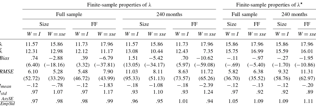
9.1.1 C–CAPM. Table 2 reports results for the one-factor (C–CAPM) case for theλandλ⋆estimates. The table presents population values for the risk premia, average risk premium es-timates, biases, and RMSEs. For ease of comparison, we report risk premia as percentages of the population standard devia-tion of the corresponding mimicking-portfolio excess return. Given the results of Section 3, this means that the reference values for the CSR–GLS estimates and theλ⋆estimates are the same, whereas the reference values for CSR–OLS estimates and CSR–GLS/λ⋆estimates differ. This is because the same popu-lation risk premium is divided by different popupopu-lation values of the standard deviations of the mimicking-portfolio excess re-turns. Biases and RMSEs are reported as percentages of the population standard deviation of the corresponding mimicking-portfolio excess return, and also as percentages of the popula-tion absolute values of the risk premia (in parentheses).
Table 2. λversusλ⋆
Finite-sample properties ofλ Finite-sample properties ofλ⋆
Full sample 240 months Full sample 240 months
Size FF Size FF Size FF Size FF
W=I W=sse W=I W=sse W=I W=sse W=I W=sse W=I W=sse W=I W=sse
λ 11.57 15.86 11.73 17.96 11.57 15.86 11.73 17.96 15.86 17.96 15.86 17.96 ˆ
λ 12.31 12.98 12.12 11.17 13.08 10.44 12.43 7.35 15.75 16.99 15.59 16.01
Bias .74 −2.88 .39 −6.79 1.51 −5.42 .70 −10.62 −.11 −.97 −.27 −1.95
(6.40) (−18.16) (3.32) (−37.81) (13.05) (−34.17) (5.97) (−59.08) (−.69) (−5.40) (−1.70) (−10.86)
RMSE 6.10 5.28 5.48 7.90 11.03 8.11 8.63 11.72 5.82 6.38 9.32 11.31
(52.72) (33.29) (46.72) (43.99) (95.33) (51.13) (73.57) (65.26) (36.70) (35.52) (58.76) (62.97)
tmean −.12 −.78 −.12 −1.83 −.18 −1.08 −.18 −2.39 −.12 −.13 −.12 −.20
tstd .97 1.07 .97 1.17 .93 1.10 .93 1.24 .97 .92 .92 .89
AsySE
EmpStd .97 .98 .98 .99 .96 .95 1.01 .94 1.05 1.09 1.09 1.11
NOTE: Here we simulate a one-factor C–CAPM economy 10,000 times under the null (with theαparameters set to 0). Parameter estimates of the LFM are obtained using GMM withW=I. In the bootstrap, we simulate jointly the factor and the residuals from the estimated LFM. We consider two lengths of the data set: the full sample of 525 observations (full sample) and a shorter sample of 240 observations (240 months). We consider 2 choices of assets: the 10 size portfolios (size) and the 25 FF portfolios (FF). When investigating the properties of estimates of the LFM, we consider estimates based on the two weighting matrices,W=IandW=see= ˆ−1
ee. Estimates of the parameters of the LFM⋆are obtained by
exactly identified GMM. Asymptotic statistics are obtained assuming no serial correlation. The first row reports the population value of the risk premium as a percentage of the population standard deviation of the excess return on the corresponding mimicking portfolio. The second row reports the average value across simulations of the risk premium as a percentage of the population standard deviation of the excess return on the corresponding mimicking portfolio. The third and fourth rows report absolute (percentage) bias and absolute (percentage) RMSEs. The fifth and sixth rows report the means and standard deviation of thet-ratios across simulations. The seventh row reports the ratio between average asymptotic standard errors across simulations and empirical standard deviation.
Table 2 also reports averages and standard deviations of as-ymptotict-ratios on the risk premium estimates. We computet -ratios using the population risk premium as the reference value. Finally, the table reports the ratios between the average asymp-totic standard error on the risk premium estimate and the stan-dard deviation of the estimate across simulations.
LFM. First, consider the results for the estimates ofλ. OLS estimates are biased away from 0, with biases ranging from .39 to 1.51 and percentage biases ranging from 3.32% to 13.05%. In contrast, GLS estimates are biased toward 0, with biases rang-ing from−10.62 to−2.88 and percentage biases ranging from
−59.08% to−18.16%. In all instances, the absolute percentage bias is larger for the GLS estimates than for the OLS estimates. RMSEs are substantial for both estimators, ranging from 5.48 to 11.03 (46.72–95.33% of the true value) for the OLS estima-tor and from 5.28 to 11.72 (33.29–65.26% of the true value) for the GLS estimator. Percentage RMSEs are always larger for the OLS estimator than for the GLS estimator. As would be expected, reducing the length of the sample increases biases and RMSEs. Using the FF rather than the size portfolios leads to smaller (larger) biases and RMSEs for the OLS (GLS) esti-mates. In this exercise, as well as in the other exercises that use nonoverlapping data, going from the iid bootstrap to the block bootstrap (not reported in the table, but available in a separate appendix) makes little difference.
Asymptotict-ratios have means substantially different from 0, ranging from−2.39 to−.12; the biases are always more pro-nounced for the GLS estimator than for the OLS estimator. The standard deviations of the asymptotict-ratios also can deviate substantially from the theoretical value of 1, ranging from .93 to 1.24. The deviations are always more pronounced for the GLS estimator than for the OLS estimator. Finally, the ratios between asymptotic and empirical standard deviations are mainly<1 for both choices of weighting matrix, ranging from .95 to 1.01, with no clear superiority of one estimator over the other.
LFM⋆. Results for the estimates of λ⋆ can be directly compared with the results for the CSR–GLS estimates, because the population Sharpe ratios for the two mimicking portfolios are the same. There is an advantage in using the LFM⋆ formula-tion in terms of bias: Absolute biases of theλ⋆estimates are al-ways substantially smaller than the biases of the corresponding CSR–GLS estimates. For example, for the 240-month sample FF portfolios, the bias for the CSR–GLS estimator is−10.62, whereas that for theλ⋆ estimator is only−1.95. Note that un-der normality, the estimates ofλ⋆ should be unbiased (Dickey 1967); Thus, deviations from normality (e.g., skewness and ex-cess kurtosis) in our bootstrap data are responsible for the biases that we document. RMSEs are roughly of the same magnitude as those for the GLS estimates.
Percentage biases for theλ⋆ estimator range from−10.86% to−.69% and are higher or lower than the percentage biases for the CSR–OLS estimates depending on the choice of test assets. Percentage RMSEs for theλ⋆ estimator range from 35.52% to 62.97%, again higher or lower than the corresponding quanti-ties for the CSR–OLS estimates depending on the choice of test assets. Thus the performance of theλ⋆and CSR–OLS estimates in terms of bias and RMSE is roughly comparable.
T-ratios in the LFM⋆ are negatively biased. Biases are sim-ilar to those for the OLS estimates and much less pronounced than those for the GLS estimates. The standard deviations of the t-ratios are consistently<1, also similar to the OLS estimates. Finally, the ratios between asymptotic standard errors and em-pirical standard errors are consistently>1, differing from the OLS and GLS estimates.
9.1.2 I–CAPM. We also performed our simulation analy-sis for the multifactor (I–CAPM) case. Results for this case are not reported in Table 2 but are available in a separate appendix. In this case we focus on the risk premia on the nontraded factor: changes in the dividend yield.
Consider first the simulation evidence for the LFM formu-lation. As in the one-factor case, the GLS estimates are biased toward 0 (the bias is positive, whereas the true value of the pa-rameter is negative); in contrast, the bias in the OLS estimates changes sign depending on the set of assets. Again as in the one-factor case, percentage biases are more pronounced for the GLS estimates. Percentage RMSEs are substantial for both sets of estimates and of roughly similar magnitude. Consistent with the one-factor case, RMSEs are always larger for the OLS es-timates than for the GLS eses-timates. Biases int-ratios are now consistently positive for both estimators; as in the one-factor case, they are more pronounced for the GLS estimator. As in the one-factor case, standard deviations oft-ratios are <1 for the OLS estimator and>1 for the GLS estimator. Finally, the ratios between asymptotic and empirical standard errors of the estimates are mainly <1, also consistent with the one-factor case.
Consider now the simulation evidence for the LFM⋆ formu-lation. As in the one-factor case,λ⋆estimates are biased toward 0; thus biases are now positive. Again, biases are consistently smaller than for the corresponding GLS estimates. RMSEs are again comparable to those for the GLS estimates. Comparing
λ⋆estimates to CSR–OLS estimates, we see that the percentage biases are always more pronounced for theλ⋆ estimates. Per-centage RMSEs, in contrast, are similar for the two estimators, with their relative size depending on the choice of test assets, just as in the one-factor case. Biases int-ratios are positive, but less pronounced than for the CSR–OLS estimator and compa-rable to that for the CSR–GLS estimator, as in the one-factor case. The volatilities of thet-ratios are now consistently>1, and when comparing departures from the true value of 1, no one estimator clearly outperforms the other two estimators. Fi-nally, the ratios between asymptotic and empirical standard er-rors of the estimates are always>1 and tend to depart from the reference value of 1, more so than the other two estimators, consistent with the one-factor case.
9.1.3 Summary and Discussion. In summary, the various scenarios herein considered paint a fairly consistent picture of the advantages and disadvantages of the various estimators. In terms of bias, theλ⋆estimates always do better than the CSR– GLS estimates, whereas they often do worse than the CSR– OLS estimates. In terms of RMSE, theλ⋆estimates always do better than the CSR–OLS estimates and perform similarly to the CSR–GLS estimates. In terms of average t-ratios, the λ⋆
estimates always do better than the CSR–GLS estimates and perform similarly to the CSR–OLS estimates.
We can compare the foregoing results with the results ob-tained by Chen and Kan (2006) in a similar setting. Chen and Kan analytically derived the small-sample bias and standard de-viation of CSR estimates for the OLS and GLS cases under the assumption of iid Gaussian returns and factor, and they per-formed a simulation exercise for nonnormal (Studentt) returns and factor. They considered the case in which the factor is cal-ibrated to consumption growth and considered both size-sorted and size- and value-sorted test portfolios. Several of their re-sults are consistent with ours. They found that absolute biases were larger for the GLS estimates than for the OLS estimates, that the GLS estimates were consistently biased toward 0, and that the sign of the bias for the OLS estimates could be either
positive or negative, depending on the calibration. They found that the GLS estimates were less volatile than the OLS esti-mates, which is consistent with our finding that the RMSEs are smaller for the GLS estimates.
9.2 Changing Betas
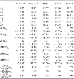
In this section we further investigate the nature of the differ-ence in results between the LFM and LFM⋆ formulations. We replicate the one-factor case for the scenario with the full sam-ple and size portfolios, but with the betas with respect to con-sumption growth scaled by a factorm. The variances of the idio-syncratic components are adjusted so that the variances of re-turns remain the same. Thus, as betas increase in absolute value, the percentages of return variance explained by the single-index model also increase.
The results, reported in Table 3, clearly show how the bi-ases in the λestimates tend to 0 as the consumption betas in-crease from 1/3 to 3 times the original value. This pattern is especially pronounced for the CSR–GLS estimate, the bias of which goes from−11.22 to−.43 (from−68.62% to−3.36%). On the other hand, the bias in theλ⋆estimates remains remark-ably stable (between −.32 and−.11; −1.96% and−.69% of
NOTE: Here we simulate a C–CAPM economy 10,000 times under the null (with theα
parameters set to 0). Parameter estimates of the LFM are obtained using GMM withW=I for different values ofβ. We denote these different values ofβwithβadj=m∗β, wherem
is a scalar. In the bootstrap, we jointly simulate the factor and the residuals from the esti-mated LFM. The adjusted returns that we construct have the same volatility as the original returns. The columns report simulation results for the cases ofm=1/3,1/2,1,2,3. We in-vestigate the properties of estimates of the LFM using the full sample of 525 observations, the 10 size portfolios (size), and the 2 weighting matrices,W=IandW= ˆ−ee1.
Esti-mates of the parameters of the LFM⋆are obtained by exactly identified GMM. Asymptotic
statistics are obtained assuming no serial correlation. We report the population value of the risk premium as a percentage of the population standard deviation of the excess re-turn on the corresponding mimicking portfolio, the average value across simulations of the risk premium as a percentage of the population standard deviation of the excess return on the corresponding mimicking portfolio, absolute (percentage) bias and absolute (percent-age) RMSEs, mean and standard deviation of thet-ratios across simulations, and the ratio between average asymptotic standard errors across simulations and empirical standard de-viation.
the population values) across values of m. As in the scenar-ios described in the previous section, the percentage RMSEs of the CSR–GLS andλ⋆estimates are comparable, whereas the percentage RMSEs of the CSR–OLS estimator are consistently higher. RMSEs also decrease monotonically as the consump-tion betas increase (in absolute value), although they are still substantial form=3, ranging from 34.04% to 44.56%.
In summary, we conclude that the discrepancies in results across the different risk premium estimators tend to disappear as the factor explains more of the variance in returns.
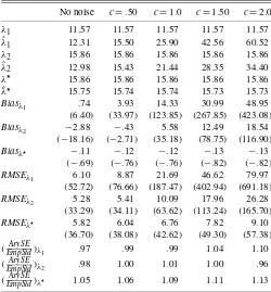
9.3 Noisy Factor
Table 4 gives results for the one-factor case when the fac-tor is observed with noise. We focus on one scenario only: full sample and size portfolios. Following Kan and Zhou (1999), we consider noise with standard deviations equal to .5, 1, 1.5, and 2 times the standard deviation of the factor.
A setting in which the issue of measurement error in the fac-tor arises naturally is that of tests of heterogenous-agent models (see, e.g., Brav, Constantinides, and Geczy 2002; Jacobs and Wang 2004). In these studies, the realizations of the factors are
Table 4. Noisy factor:λ1(W=I),λ2(W= ˆee−1) versusλ⋆ No noise c=.50 c=1.0 c=1.50 c=2.0
λ1 11.57 11.57 11.57 11.57 11.57
ˆ
λ1 12.31 15.50 25.90 42.56 60.52
λ2 15.86 15.86 15.86 15.86 15.86
ˆ
λ2 12.98 15.43 21.44 28.35 34.40
λ⋆ 15.86 15.86 15.86 15.86 15.86 ˆ
λ⋆ 15.75 15.74 15.74 15.73 15.73
Biasλ1 .74 3.93 14.33 30.99 48.95 (6.40) (33.97) (123.85) (267.85) (423.08)
Biasλ2 −2.88 −.43 5.58 12.49 18.54 (−18.16) (−2.71) (35.18) (78.75) (116.90)
Biasλ⋆ −.11 −.12 −.12 −.13 −.13
(−.69) (−.76) (−.76) (−.82) (−.82)
RMSEλ1 6.10 8.87 21.69 46.62 79.97 (52.72) (76.66) (187.47) (402.94) (691.18)
RMSEλ2 5.28 5.41 10.09 17.96 26.28 (33.29) (34.11) (63.62) (113.24) (165.70)
RMSEλ⋆ 5.82 6.04 6.76 7.82 9.10
(36.70) (38.08) (42.62) (49.30) (57.38) (EmpStdAsySE )λ1 .97 .99 .99 1.04 1.10 (EmpStdAsySE )λ2 .98 1.00 1.01 1.00 .96 (EmpStdAsySE )λ⋆ 1.05 1.06 1.09 1.11 1.13
NOTE: Here we simulate a C–CAPM economy 10,000 times under the null (with the
αparameters set to 0). Parameter estimates of the LFM are obtained using GMM with W=I. In the bootstrap, we jointly simulate the factor and the residuals from the estimated LFM. For each bootstrap replication, we add an iid Gaussian shock to the factor. The stan-dard deviation of the shock is proportional (constant of proportionality equal toc) to the population standard deviation of the factor. The columns report simulation results for the case of no noise and the case of noise (c=.5,1,1.5,2.0). We investigate the properties of estimates of the LFM using the full sample of 525 observations, the 10 size portfolios (size), and the 2 weighting matrices,W=IandW= ˆ−ee1. Estimates of the parameters of the LFM⋆are obtained by exactly identified GMM. Asymptotic statistics are obtained
assuming no serial correlation. We report the population value of the risk premium as a percentage of the population standard deviation of the excess return on the correspond-ing mimickcorrespond-ing portfolio, the average value across simulations of the risk premium as a percentage of the population standard deviation of the excess return on the corresponding mimicking portfolio, absolute (percentage) bias and absolute (percentage) RMSEs, mean and standard deviation of thet-ratios across simulations, and the ratio between average asymptotic standard errors across simulations and empirical standard deviation.
the moments of the cross-sectional distribution of consumption growth. Because the cross-sections used in these studies are relatively small, the cross-sectional moments can be estimated with a great deal of noise.
The table presents reference values of the risk premia, bi-ases, RMSEs, and ratios between average asymptotic standard errors and empirical standard deviations of the estimates. In this setting, the results dramatically favor the LFM⋆ formula-tion over both the CSR–OLS and CSR–GLS approaches. Bias and RMSE monotonically increase with noise for the CSRλ
estimates. For example, when the noise is twice as large as the signal, the biases for the CSR–OLS and CSR–GLS estimates are 48.95 and 18.54 (423.08% and 116.90%) and RMSEs are as high as 79.97 and 26.28 (691.18% and 165.70%). In con-trast the bias for theλ⋆ estimates never exceeds .13 (.82%) in absolute value, with a maximum RMSE of 9.10 (57.38%).
9.4 Estimates of Betas
Here we analyze the finite-sample properties ofβ andβ⋆. Note that theβ⋆estimates are subject to the errors-in-variables (EIV) problem arising from estimation of the weights of the maximum-correlation mimicking portfolio. We conduct simu-lations to assess the magnitude of this bias.
Table 5 reports results for the C–CAPM case. We report the same statistics as in Table 2, averaged across assets. For ease of comparison, bothβandβ⋆estimates are scaled by the ratio between the population standard deviations of the factor and of the dependent variable; thus they have the dimension of corre-lation coefficients. Percentage biases and RMSEs are computed as average biases and RMSEs across assets divided by the pop-ulation values of the betas, averaged across assets.
In the results for the estimates of β, biases are essen-tially nonexistent, although RMSEs are substantial (as high as 38.48%). Similarly unbiased on average, are thet-ratios. The volatilities of thet-ratios are close to 1, and the ratios between average the asymptotic standard errors and empirical standard errors are also close to 1.
In the results for the estimates of β⋆, biases are negative (the well-known “attenuation bias” associated with the EIV problem) and substantial, ranging from −29.67 to −12.18 (−53.30% to−17.53%). RMSEs also are substantial, as high as 31.63 (56.82%), although of the same order of magnitude as for the LFM specification. Finally, biases int-ratios are neg-ative and pronounced, and there are substantial discrepancies between small-sample and asymptotic volatilities oft-ratios.
We also perform our analysis for the case of the I–CAPM (results not reported in the table). In this case we focus on the betas for the nontraded factor. As in the single-factor case, bi-ases and RMSEs are more pronounced for theβ⋆estimates than for theβestimates.
9.5 Size and Power of the Tests
We investigate, by simulation, the size and power proper-ties of the Wald-style tests for the one-factor and two-factor models. Our main contribution is an analysis of the size and
Table 5. βversusβ⋆
Finite-sample properties ofβ Finite-sample properties ofβ⋆
Full sample 240 months Full sample 240 months
Size FF Size FF Size FF Size FF
β 17.92 16.27 17.92 16.27 69.47 55.67 69.47 55.67 ˆ
β 17.80 16.26 17.70 16.29 57.29 37.00 46.50 26.00
Bias −.12 −.01 −.22 .02 −12.18 −18.67 −22.97 −29.67
(−.67) (−.06) (−1.23) (−.12) (−17.53) (−33.54) (−33.06) (−53.30)
RMSE 4.22 4.24 6.25 6.26 17.73 21.69 27.88 31.63
(23.55) (26.06) (34.88) (38.48) (25.52) (38.96) (40.13) (56.82)
tmean −.01 −.02 −.01 −.02 −1.14 −1.83 −1.71 −2.99
tstd 1.02 1.02 1.03 1.03 1.15 1.31 1.31 1.72
AsySE
EmpStd .98 .98 .98 .98 1.07 1.11 1.11 1.10
NOTE: Here we simulate a one-factor C–CAPM economy 10,000 times. Parameter estimates of the LFM are obtained using GMM withW=I. In the bootstrap, we jointly simulate the factor and the residuals from the estimated LFM. We consider 2 lengths of the data set: the full sample of 525 observations (full sample) and a shorter sample of 240 observations (240 months). We consider 2 choices of assets: the 10 size portfolios (size) and the 25 FF portfolios (FF). Estimates of the parameters of the LFM⋆are obtained by exactly identified
GMM. Asymptotic statistics are obtained assuming no serial correlation. Bothβandβ⋆estimates (averageβ’s andβ⋆’s across simulations and across assets) are scaled by the ratio
between the population standard deviations of the factor and the excess return. We report population and average values of the betas, absolute (percentage) bias and absolute (percentage) RMSEs, mean and standard deviation of thet-ratios across simulations, and the ratio between average asymptotic standard errors across simulations and empirical standard deviation.
power properties of tests in the context of the LFM⋆ represen-tation.
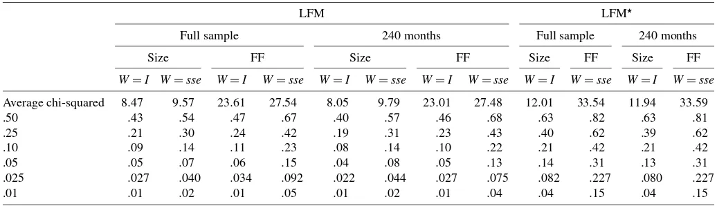
9.5.1 Size. Table 6 reports the theoretical and actual sizes of the Wald-style test for the one-factor model the for LFM and LFM⋆ specifications. First, consider the results for the LFM specification for the full sample. The actual size is generally close to the theoretical value, although there are systematic dis-crepancies. The CSR–OLS approach always leads to lower re-jection rates than the CSR–GLS approach, and using the FF portfolios leads to higher rejection rates than using the size-sorted portfolios. Results are similar for the shorter sample of 240 months. Indeed, rejection rates are quite similar for the two sample lengths. Results are also similar for the block bootstrap (not reported in the table).
When we consider the LFM⋆ specification, overall we see overrejections. Again, rejections are stronger for the FF port-folios. Rejection rates for the LFM⋆ specification are always
higher than rejection rates for the LFM specification for both the OLS and GLS approaches.
Results for the I–CAPM (not reported in the table) are similar to those for the one-factor specification.
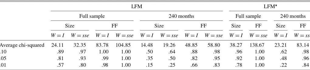
9.5.2 Power. Table 7 (organized similarly to Table 6) re-ports rejection rates for the Wald test under the alternative, where the size is adjusted using the bootstrap results of Table 6. We compute the 10%, 5%, and 1% quantiles of the empirical distribution of the Wald statistic under the null and compute the percentage of times that the Wald statistic exceeds the corre-sponding quantile, when the economy is simulated under the alternative.
In the case of the LFM specification, the power of the tests is higher forW= ˆee−1, for the FF portfolio returns, and for the longer sample. For example, consider the case of the full sample and size-sorted portfolios. When the size is set at 1%, the actual rejection rate is 57% for the OLS approach; the rejection rate increases to 80% for the GLS approach, further increases to
Table 6. Size of the Wald test
LFM LFM⋆
Full sample 240 months Full sample 240 months
Size FF Size FF Size FF Size FF
W=I W=sse W=I W=sse W=I W=sse W=I W=sse W=I W=sse W=I W=sse
Average chi-squared 8.47 9.57 23.61 27.54 8.05 9.79 23.01 27.48 12.01 33.54 11.94 33.59
.50 .43 .54 .47 .67 .40 .57 .46 .68 .63 .82 .63 .81
.25 .21 .30 .24 .42 .19 .31 .23 .43 .40 .62 .39 .62
.10 .09 .14 .11 .23 .08 .14 .10 .22 .21 .42 .21 .42
.05 .05 .07 .06 .15 .04 .08 .05 .13 .14 .31 .13 .31
.025 .027 .040 .034 .092 .022 .044 .027 .075 .082 .227 .080 .227
.01 .01 .02 .01 .05 .01 .02 .01 .04 .04 .15 .04 .15
NOTE: Here we simulate a one-factor C–CAPM economy 10,000 times under the null (with theαparameters set to 0). Parameter estimates of the LFM are obtained using GMM withW=I. In the bootstrap, we jointly simulate the factor and the residuals from the estimated LFM. We consider two lengths of the data set: the full sample of 525 observations (full sample) and a shorter sample of 240 observations (240 months). We consider 2 choices of assets: the 10 size portfolios (size) and the 25 FF portfolios (FF). When we investigate the properties of estimates of the LFM, we consider estimates based on the two weighting matrices,W=IandW=see= ˆee−1. Estimates of the parameters of the LFM⋆are obtained by exactly identified GMM. Asymptotic statistics are obtained assuming no serial correlation. We report the theoretical and actual sizes of the Wald test for the one-factor model. For the LFM and LFM⋆specifications. The LFM test statistic should beχN2−Kdistributed, whereas the LFM⋆test statistic should beχN2distributed.
Table 7. Power of the Wald test
LFM LFM⋆
Full sample 240 months Full sample 240 months
Size FF Size FF Size FF Size FF
W=I W=sse W=I W=sse W=I W=sse W=I W=sse W=I W=sse W=I W=sse
Average chi-squared 24.11 32.35 83.78 104.85 14.48 19.26 48.85 58.80 38.27 138.67 23.21 83.14
.10 .89 .97 1.00 1.00 .50 .64 .88 .98 .96 1.00 .62 .98
.05 .81 .93 .99 1.00 .35 .50 .82 .95 .92 1.00 .48 .96
.01 .57 .80 .98 1.00 .15 .25 .66 .83 .78 1.00 .22 .84
NOTE: Here we simulate a one-factor C–CAPM economy 10,000 times under the alternative (α=0). Parameter estimates of the LFM are obtained using GMM withW=I. In the bootstrap, we jointly simulate the factor and the residuals from the estimated LFM. We consider two lengths of the data set: the full sample of 525 observations (full sample) and a shorter sample of 240 observations (240 months). We consider 2 choices of assets: the 10 size portfolios (size) and the 25 FF portfolios (FF). When we investigate the properties of estimates of the LFM, we consider estimates based on the two weighting matrices,W=IandW=see= ˆ−1
ee. Estimates of the parameters of the LFM⋆are obtained by exactly identified GMM.
Asymptotic statistics are obtained assuming no serial correlation. We report rejection rates for the Wald test under the alternative, where the size is adjusted using the bootstrap results of Table 6. We compute the 10%, 5%, and 1% quantiles of the empirical distribution of the Wald statistic under the null, then compute the percentage of times the Wald statistic exceeds the corresponding quantile when the economy is simulated under the alternative.
98% for the choice of FF test portfolios, and decreases to 15% when the sample is shortened to 240 months.
In the case of the LFM⋆ specification, the power is also
higher for the FF portfolio returns and for the longer sample. For example, in the case of the entire sample, for size portfo-lios, when the size is set at 1%, the rejection rate is 78%; the rejection rate increases to 100% for the FF portfolios, and falls to 22% for the shorter sample. The power of the LFM⋆ specifi-cation is always higher than the power of the LFM specifispecifi-cation and the OLS approach and comparable to the power of the GLS approach.
Results for the I–CAPM (not reported in the table) are simi-lar. In the case of the LFM specification, the power of the tests is almost always higher forW= ˆee−1, although the differences are modest. Power also is higher for tests using the FF portfolios and for the longer sample. The power of the LFM⋆specification is comparable to the power of the LFM specification with the GLS approach and always higher than the power of the LFM specification with the OLS approach.
Thus, when it comes to power, the CSR–GLS and LFM⋆ ap-proaches have an advantage over the CSR–OLS approach, es-pecially in the one-factor case. Moreover, there is a clear ad-vantage to using the larger cross-section of the FF portfolios in both the one-factor and the two-factor cases.
10. EXTENSIONS
In this section we consider several extensions of our main analysis. First, we consider the case of time-varying condi-tional moments and condicondi-tional versions of the LFM and LFM⋆ formulations. Second, we consider an alternative approach to the construction of mimicking portfolios, first suggested by Lehmann and Modest (1988). Third, we consider the perfor-mance of the correction for small-sample bias in risk premium estimates, suggested by Chen and Kan (2006). Fourth, we study the performance of the various methods when we consider long-horizon overlapping returns. Finally, we consider the implica-tions of the restricimplica-tions from the LFM and LFM⋆formulations
on covariance matrices for the purpose of portfolio construc-tion. Details of the various exercises are in a separate appendix available on request. In what follows we provide summaries of the various setups and results.
10.1 Conditional Models
Here we consider conditional versions of the LFM and LFM⋆ formulations. We allow for both risk premia and betas to be time-varying, but also specialize the analysis for cases in which betas or risk premia are constant. Following Ferson and Har-vey (1999), we assume that the conditional betas and the condi-tional expectations of the factors are linear in the instruments. Also, following Ferson and Harvey (1991), we assume that the conditional risk premia also are linear in the instruments. For tractability, we assume that although the betas are time-varying, the factors are homoscedastic. The same assumption is made in, for example, the simulation analysis of Ferson et al. (2005). We focus on conditional versions of the I–CAPM, where the non-traded factor is the innovation in the dividend yield and lagged realizations of the dividend yield drive the time-varying betas and dividend yield risk premium. Conditional betas with respect to the traded factor, the market, also can vary as a function of the dividend yield.
Relative to the unconditional case, the properties of all esti-mators worsen considerably when the betas are allowed to vary. For example, the percentage bias of the CSR–OLS estimate in-creases from−3.69% to 79.88% and the percentage RMSE in-creases from 67.44% to 193.91%, where the population value of the Sharpe ratio is−7.94%. In contrast, when the betas are kept constant, the results are comparable to the base case illus-trated in Table 2. In terms of the relative performance of the three estimators, the CSR–OLS estimator still displays the low-est bias, but the highlow-est RMSE, across scenarios. Theλ⋆ esti-mate displays the lowest percentage RMSE when the betas are time-varying. The CSR–GLS estimator has the lowest percent-age RMSE when the betas are constant.
Interestingly, while the properties of the estimates worsen, the correlations between mimicking-portfolio returns and the factor can increase substantially. For example, in the case where betas and risk premia are both time-varying, the correlations for the conditional mimicking portfolios are 18.76% for CSR– OLS, 26.83% for CSR–GLS, and 26.50% for maximum cor-relation. For comparison, the respective correlations for the unconditional mimicking portfolios are 16.69%, 20.76%, and 20.76%.
10.2 Lehmann and Modest Portfolios
Lehmann and Modest (1988; LM hereinafter) argued that constructing unit-beta mimicking portfolios tends to place large weights on security returns associated with large estimated be-tas. Although this procedure is appropriate in the absence of measurement error, it is less appropriate when estimated betas reflect both the true betas and measurement error. Thus LM sug-gested constructing portfolios with minimum idiosyncratic risk, with betas of 0 with respect to all factors other than the factor being tracked and with the unit-beta constraint replaced by the constraint that the sum of portfolio weights equals 1. LM ap-proximated theˆeematrix with a diagonal matrix consisting of estimates of the idiosyncratic variances,Dσˆe. We also consider a further approximation, in which all of the variances are the same,Iσˆe2. Note that because the LM portfolios do not have a beta of 1, we divide the portfolio excess cash flows by the port-folio beta to obtain estimates of the factor risk premium. We perform this analysis for both the C–CAPM and the I–CAPM.
In general, the LM approach does worse than the LFM⋆ for-mulation, both in terms of bias and RMSE. In the case of the C–CAPM, for example, the LM procedure leads to percentage biases of 8.12% (W=I) and 7.19% [W =(Dσˆe)
−1], with
re-spective population values of the Sharpe ratios of 11.59% and 11.57%. For a comparison, theλ⋆estimate has a bias of−.69%. Percentage RMSEs are 55.73% and 53.51% for the LM portfo-lios and 36.70% for the maximum-correlation portfolio.
10.3 Bias Corrections
Chen and Kan (2006) derived the small-sample distribution of the estimates of λ for both the OLS and the GLS cases under the assumption of Gaussian returns. In addition, they showed that the adjustments suggested by Litzenberger and Ra-maswamy (1979) and Kim (1995), based on asymptotic results, lead to bias-adjusted estimators without finite moments.
Here we study the small-sample properties of the bias-adjusted estimators proposed by Chen and Kan (2006). We replicate the simulation analysis presented in Table 2 of the article for the case of the iid bootstrap. These estimators re-duce the bias in 8 of our 16 cases. This result differs from that of Chen and Kan, who found that for the most part, the bias-adjusted estimates have less bias than the standard estimates in simulations. We attribute the difference in results to the fact that Chen and Kan assume that returns and factors are either multi-variate normal or multimulti-variatet-distributed, whereas we sample from the empirical distribution. Moreover, the RMSEs of the bias-adjusted estimates increase substantially, especially for the shorter sample of 240 months. For example, in the case of the C–CAPM, size portfolios,W=I, the RMSE is 95.33% for the standard estimate and 211.91% for the bias-adjusted estimate. This result is in line with the substantial increase in standard deviation of the bias-adjusted estimates documented by Chen and Kan, especially for the CSR–GLS case.
Comparing theλ and the λ⋆ estimates, the introduction of bias adjustment means that now there are cases in which the CSR–GLS estimator has less bias than theλ⋆estimator. (With-out a bias adjustment, the CSR–GLS estimator always has more bias than theλ⋆ estimator.) On the other hand, there are cases in which theλ⋆ estimator has less bias than the bias-adjusted
CSR–OLS estimator. Finally, the λ⋆ estimates always have a lower RMSE thanboththe bias-adjusted CSR–OLS and CSR– GLS estimates.
In summary, in terms of bias, the bias-adjustment of Chen and Kan (2006) does not significantly alter the comparison be-tween the LFM and LFM⋆formulations. In terms of RMSE, the bias adjustment makes theλestimates always noisier than the
λ⋆estimates.
10.4 Long-Horizon Returns
Some authors have suggested that studying long-horizon re-turns may help better characterize the explanatory power of asset-pricing models, especially in the case of the C–CAPM (see, e.g., Lynch 1996; Daniel and Marshall 1997; Gabaix and Laibson 2001; Jagannathan and Wang 2007). Thus, we perform a simulation exercise where we simulate an iid economy at the monthly frequency, but study the inference on the factor risk premia using quarterly and annual returns. We perform the sim-ulation for both the C–CAPM and the I–CAPM.
As would be expected, our results generally deteriorate rela-tive to the case of monthly returns. Yet, at least in the case of the C–CAPM, the deterioration is much less marked for theλ⋆
estimates than for the CSR estimates. For example, consider the case of annual returns. The percentage biases in the CSR–OLS and CSR–GLS estimates are−10.43% and−66.55%, with re-spective population values of the Sharpe ratios of 11.57% and 15.86%. For comparison, the corresponding percentage biases in the case of monthly returns are 6.40% and−18.16%. (Given the assumption of iid returns, the population values are the same as in the case of annual returns.) Similarly, percentage RM-SEs are 114.62% and 70.40% in the case of annual returns and 52.72% and 33.29% in the case of monthly returns. There is much less deterioration in the properties of the λ⋆ estimates. Percentage bias and RMSE are−.57% and 43.28% in the case of annual returns and−.69% and 36.70% in the case of monthly returns, with a population Sharpe ratio of 15.85%. Thus, using long-horizon returns may get around issues of misalignment between consumption decisions and returns in tests of the C– CAPM, but also may worsen considerably the properties of the risk premium estimators, particularly those based on the con-struction of unit-beta portfolios.
10.5 Portfolio Implications
The previous sections have focused on the implications of the LFM and LFM⋆ representations formeanestimates of risk premia. It is now interesting to explore whether the two repre-sentations also have different implications for the covariance structure in asset returns for the purpose of constructing mean– variance–efficient portfolios. Specifically, we can take an “APT view” of the factorsyt andy⋆t, and approximate the covariance matrices ˆee andˆe⋆e⋆ withDσˆ
e andDσˆe⋆. We can then use the resulting approximate covariance matrices as inputs for the construction of mean–variance–efficient portfolios.
We construct global minimum-variance (GMV) portfolios and evaluate their out-of-sample performance. Following the methodology of Jagannathan and Ma (2003), we estimate the