Full Terms & Conditions of access and use can be found at
http://www.tandfonline.com/action/journalInformation?journalCode=ubes20
Download by: [Universitas Maritim Raja Ali Haji] Date: 13 January 2016, At: 01:03
Journal of Business & Economic Statistics
ISSN: 0735-0015 (Print) 1537-2707 (Online) Journal homepage: http://www.tandfonline.com/loi/ubes20
A Stochastic Frontier Analysis of Financing
Constraints on Investment
Hung-Jen Wang
To cite this article: Hung-Jen Wang (2003) A Stochastic Frontier Analysis of Financing
Constraints on Investment, Journal of Business & Economic Statistics, 21:3, 406-419, DOI: 10.1198/073500103288619016
To link to this article: http://dx.doi.org/10.1198/073500103288619016
View supplementary material
Published online: 01 Jan 2012.
Submit your article to this journal
Article views: 222
View related articles
A Stochastic Frontier Analysis of Financing
Constraints on Investment: The Case
of Financial Liberalization in Taiwan
Hung-Jen W
ANGThe Institute of Economics, Academia Sinica, Taipei 115, Taiwan (hjwang@econ.sinica.edu.tw)
It is shown that investment under nancing constraints can be modeled as a one-sided deviation from a frictionless investment level, and that effects of nancing constraints can be identied and quantied by imposing a distributional assumption on the effects. Panel data on Taiwanese manufacturing rms be-tween 1989 and 1996 are used in the estimation. It is found that (1) some of the sorting criteria used in the literature do not have signicant and monotonic relationships with the degrees of nancing constraint, re-sulting in problematic sample separations, and (2) the effects of nancial liberalization in Taiwan are such that the investment efciency improved over time for a typical rm, and the improvement was particularly large for smaller rms.
KEY WORDS: Financial liberalization; Financing constraints; Stochastic frontier.
1. INTRODUCTION
Over the past decades, many studies have been devoted to providing evidence for the hypothesis of nancing constraints on investment (see Chirinko 1993 and Hubbard 1998 for exten-sive reviews). According to this hypothesis, the capital market is imperfect owing to informational problems, and as such, cor-porate capital investment is no longer determined solely by fun-damentals such as user costs or Tobin’sQ, but also by nancial factors. In particular, investment is constrained if market imper-fections exert difculties for nancing investment. Therefore, failure to take into account the effect of the nancing constraint on investment leads to misspecied empirical equations.
Efforts in the empirical modeling, however, are to some ex-tent hindered by the difculty in specifying the structural rela-tionships among the real and nancial variables in both the rm and time dimensions. For example, in linear regression mod-els (e.g., Carpenter, Fazzari, and Petersen 1994), it is not clear how nancing constraints, liquidity variables, and investment spending should enter the equation and interact with each other (Chirinko 1997). For a structural Euler equation model (e.g., Whited 1992; Hubbard, Kashyap, and Whited 1995), doubts are sometimes raised as to whether the period-by-period per-turbation method can pick up the effect of a rm for which the overall investment level is constrained in the entire sample pe-riod (Gilchrist and Himmelberg 1995; Hubbard 1998). Another problem common to either of the approaches is the use of ad hoc classication criteria to separate rms into a priori constrained and unconstrained groups. As argued by Hu and Schiantarelli (1998), the dependence on a single indicator to separate sam-ples can be risky, the implication that a rm’s nancial status does not change over time may be unrealistic, and selection of the criterion may also give rise to endogenous selection prob-lems.
This article proposes a new estimation strategy that circum-vents some of the aforementioned problems. This approach does not separate samples a priori to test investment cash ow sensitivity, and it can provide not only cross-sectional, but also intertemporal comparisons of the effect of nancing con-straints. Using the experience of nancial liberalization in
Tai-wan between 1989 and 1996 as a natural experiment, the article provides new evidence concerning the nancing constraints on investment which is otherwise unavailable.
The key to the approach herein lies in the insight that nanc-ing constraints should have asymmetric effects on a friction-less level of investment; it forces realized investment to be be-low, but never above, the frictionless neoclassical level. There-fore, identication of the constraints is achieved by imposing a one-sided distributional assumption on the effect of nancing constraints. With a neoclassical model characterizing the fron-tier investment, the level of nancing-constrainedinvestment is then estimated as a deviation from the frontier, with the option of modeling the one-sided deviation as a function of rm char-acteristics. The degree of nancing constraints can also be cal-culated using the difference between the frontier and the actual levels of investment. The econometric technique is essentially thestochastic frontierestimation, which is well studied in the relevant literature.
This approach has several advantages. First, the structural relationship between the nancial and real variables are rela-tively straightforward; that is, nancing constraints have one-sided effects on investment, and nancing constraints can be explained by a vector of observable variables. This is to be compared with the more traditional approach in which direct interactions between nancing constraints, liquidity variables, and investment spending must be modeled more elaborately. Second, the sample does not have to be split a priori. Rather, ex post quantitative measures of the effect of nancing con-straints can be obtained for each observation, and comparisons of nancing constraints can be made based on these measures. This lifts the sample separation problem altogether and makes comparisons possible not only across groups of rms in a given time period, but also across time for all or selected groups of rms.
© 2003 American Statistical Association Journal of Business & Economic Statistics July 2003, Vol. 21, No. 3 DOI 10.1198/073500103288619016 406
The last-mentioned property (that the effects of nancing constraints can be compared over time) is of special interest in the case of Taiwanese corporate investment in the late 1980s and the 1990s, on which the empirical study herein is based. Taiwan’s nancial market was heavily regulated before the late 1980s and has since undergone a series of liberalization re-forms. For instance, the law that banned the establishment of new banks was lifted in 1991, and 18 new domestic banks had been set up by the end of 1996. Various interest rates were also deregulated during this period, including the bank loan rate in 1989 and the interbank call loan rate in 1992. The deposit rate was also deregulated, albeit in two phases, rst in 1989 and then in 1995. As a result of the reforms in the banking indus-try, the ratio of loans to private enterprises to GDP increased from .42 at the end of 1989 to .55 at the end of 1996. The stock market also underwent a series of reforms, and one of the consequences is the increase in the numbers of publicly traded rms and securities brokers. For example, the number publicly traded rms rose from 161 at the end of 1988 to 382 by the end of 1996.
This experience of nancial liberalization provides a unique opportunity for testing the nancing constraint hypothesis. If this hypothesis were true, then one would expect to see that the problem of nancing constraints attenuates over time for most of the rms, and for underprivileged rms in particular. To the author’s knowledge, this is the rst study that provides evidence of nancing constraint from both cross-sectional and intertemporal comparisons.
The rest of the article is organized as follows. Section 2 shows how investment in an imperfect capital market can be represented as a combination of frictionless investment and a one-sided constraint effect. Section 3 details the econometrics, and Section 4 describes the data. Section 5 describes the esti-mation results. Section 6 reports on a postestiesti-mation analysis carried out based on the quantitative measures of the nancing constraint effects. Section 7 concludes the article.
2. THE MODEL
This section motivates a stochastic frontier investment model from a rm’s optimization problem. The model follows from Chirinko and Schaller (1995), who showed that coefcients in a liquidity-augmentedQmodel are nonlinear functions of the rm’s characteristics and nancial positions. With some mod-ications, we show that the same model also implies that con-strained investment is a combination of frontier investment, rep-resented by aQinvestment model, and a one-sided constraint effect. Because of the lengthy derivation and the similarity with the cited one, the model is only sketched here; see referred to the work of Chirinko and Schaller (1995) for more informa-tion.
market values of the rm’s equity shares, debts, liquid assets,
and capital stocks, measured at the beginning of periodt. Be-cause it is assumed that the rm accrues revenues and pays ex-penses at the end of periodt,St¡1is multiplied by 1 plus the
in-terest raterto get the value of the shares for periodt. Therefore, the numerator measures the market value of the rm in exceed-ing the replacement cost of the rm at the beginnexceed-ing of periodt; the denominator,the replacement cost of the rm also measured at the beginning of periodt.
The market value of equity,St¡1, is obtained from the
fol-lowing optimization problem, in which managers maximize the expected discounted sum of dividends:
St¡1DmaxEt
where1is the time-invariant discount factor;K andI are the capital stock and investment, and KsD
Ps
uD¡1Iu; B and b are the stock and ow of debt, andBsDPsuD¡1bu;L andl are the stock and ow of liquid assets, and LsDPsuD¡1lu; jis the interest rate accrued from the stock of liquidity asset;
pIis the price of investment goods;T[¢] is the net revenue func-tion;i[¢] is the interest rate function;m[¢] is the function of liq-uidity, wherem[¢]DT[¢]CL;¸is the shadow value ofK;Áis the shadow value ofB; andà is the shadow value ofL.
Solutions to the foregoing maximization problem lead to
St¡1DEt
9tare dened similarly. These three variables have the follow-ing values in a dividend-maximization equilibrium:
3tDEfpIt¡TI[t].1¡im[t]Bt¡1/g; (4) 8tDEf1CTb[t].1¡im[t]Bt¡1/g; (5)
and
9tD1: (6)
Specifying the functional form of T[¢] is also necessary to derive the investment equation,
Equation (8) is a standard adjustment cost function in whichvt is a 0-mean production shock. Equation (9) is an information cost function in which0[Zt] measures the rm’s proneness to information and incentive problems and is a function of rm characteristicsZt. A rm more likely to suffer from informa-tion problems has a larger0[Zt] and, givenbt andBt¡1, incurs
higher informational costs. ThusF[¢] is a cost wedge between internal and external nance. Under the assumption of perfect capital markets,0[Zt] would be 0, and there is no informational cost of borrowing.
2.1 A Stochastic Frontier Model
With the functional forms in (4)–(9), (3) is substituted into (1) to obtain
Equation (10) shows that the rate of investment depends on a constant,Q, and on an unspecied function of nancial vari-ables and rm characteristics.
The expected investment is compared with and without -nancing constraints. If the capital market is perfect, as is as-sumed in the neoclassical framework, the information problem does not exist (0[Zt]D0), andQis a sufcient statistic of in-vestment. It can be seen from (10) that
E
That is, other things being equal, nancing constraints restrict investment below the neoclassical level. Thus the effect of cap-ital market imperfection isone-sided; it forces investment to go below, but never above, the frictionless level.
The foregoing observation suggests that the neoclassical in-vestment function effectively determines thestochastic frontier
investment,.It=Kt¡1/SF, which, by denition, denes the max-imum permissible rate of investment,
³ I
Equation (10) thus can be generalized as the difference between the frontier investment function and a nonnegative nancing constraint effect ut, with the latter being possibly parameter-ized by a function of a stochastic random error and variables affecting the rm’s ability to nance. Therefore,
It
whereZt is a vector of nonstochastic variables andwt is a ran-dom error.
3. ECONOMETRICS
The foregoing equation is expanded and generalized into the following empirical equations for a panel data:
yitD®CeXit¯QCeit; (14)
eitDvitCfiC¿t¡uit; (15)
vit» iidN.0; ¾v2/; (16) and
uit»nonnegative truncation ofN.¹it; ¾it2/: (17) Equation (14) says thatyit(i.e. the rate of investment) is a func-tion of the explanatory variableseX(i.e.Qvariable) and an error termeit. The composite erroreit consists of (a) a white noise error,vit; (b) the unobservable rm-specic effect, fi; (c) the time-specic effect,¿t; and (d) the negative of the nancing constraint effect,uit, which is a nonnegativetruncation of a nor-mal random variable with observation-specic mean and vari-ance. The effects offiand¿tare allowed to correlate with vari-ables ineX, thus treating them as “xed effects” in the panel model. The assumption of xed effect, as opposed to the ran-dom effect, is widely acknowledged in the investment litera-ture. ThusXitD[1;eXit;fi; ¿t] is dened, and the equations are
where vit anduit are independent among themselves and are also independent of Xit. The model comprising (14a), (15a), (16), and (17) is essentially a stochastic frontier model.
The econometric estimation of a stochastic frontier model was introduced by Aigner, Lovell, and Schmidt (1977) and Meeusen and van den Broeck (1977), who assumed a half-normal distribution for the one-sided error. But the assumed distribution is restrictive, because it implies that the mode of the one-sided error is at 0. Stevenson (1980) specied a model with a truncated normal distribution that has a mode not nec-essarily equal to 0. It is more general and includes the half-normal as a special case. Kumbhakar, Ghosh, and McGuckin (1991), Huang and Liu (1994), and Battese and Coelli (1995) further generalized the model so that the mode of the distribu-tion shifts with observadistribu-tion-specic variables rather than being a constant.
Our foregoing model is based on work of Kumbhakar et al. (1991), Huang and Liu (1994), and Battese and Coelli (1995) with two further extensions designed to minimize model mis-specications. The rst extension is to incorporate the rm-specic effect (fi) and the aggregate time effect (¿t) in the model. Without rm-specic effects, the model effectively treats multiple observations of the same rm as being obtained from independent samples, leaving the data’s panel nature un-exploited. As emphasized in studies by Kumbhakar (1991) and Kumbhakar and Hjalmarsson (1995), failure to include rm-specic effects in a panel stochastic frontier model is also likely to bias the estimate of the one-sided error, uit, which is one
of the most important elements of the estimation. The reason for this is because the measure ofuit is based on the compos-ite error term, which in turn is inuenced by the parameter estimates of the frontier function. The need to use time ef-fects can be argued similarly. The rm and time efef-fects are treated as xed effects in the model. Because of the truncated error distribution, one cannot take rst differences or subtract means from the data to eliminate the effects; differenced trun-cated normal distributions do not result in a known distrib-ution. Instead, the dummy variable approach is used as sug-gested in the formulation of Kumbhakar (1991). Although the dummy variable approach could be impractical for a very large number of cross-sections, with the N andT (184 and 8), one can include all of the dummies and still manage the estima-tion.
The second extension is to use a exible approach to model heteroscedasticity in uit. Whereas heteroscedasticity may af-fect estimation efciency only in a linear regression model, it leads to biased estimates in a stochastic frontier model, in which a part of the error is distributed asymmetrically (Caudill and Ford 1993; Caudill, Ford, and Gropper 1995; Hadri 1999). Because uit has a truncated normal distribution, its variance is a function of both¹it and¾it2; therefore, heteroscedasticity ofuit can be modeled through a nonconstant,¹it, a noncon-stant,¾it2, or both. The approach of Kumbhakar et al. (1991), Huang and Liu (1994), and Battese and Coelli (1995) makes
¹itobservation-specic. Caudill et al. (1995) kept¹itconstant (and equal to 0, i.e., a half-normal model) but allows¾it2to be observation-specic. The model here allows both¹itand¾it2to be observation-specic. As is shown in the estimation result, this added exibility is not redundant, but rather improves the estimation signicantly.
More specically, variables in (17) are parameterized as
¹itDc0CZit± (18)
and
¾it2Dexp.c1CZit° /; (19) wherec0 andc1 are constant andZis a vector of nonstochas-tic variables. The parameterizations specify ¹it and¾it2 to be a function of the same variables but allows for different in-tercepts and slopes. That is, it is assumed that variables af-fecting the mean of the pretruncated distribution also inuence the (log of the) variance of the distribution, although the ef-fects are not necessarily the same and could even have opposite signs.
The log-likelihood function of observationyit can be writ-ten as
andÁand8are the probability density and cumulated density functions of a standard normal distribution.
As mentioned, one of the advantages of the stochastic fron-tier estimation is the ability to obtain quantitative measures of the one-sided effects. Based on these measures, one can then calculate theinvestment efciency index(IEI), which mea-sures the extent to which a rm’s rate of investment is close to the frictionless and deterministic level. This is dened as
IEIitD.Xit¯ ¡uit/=Xit¯ if the dependent variable is in the original unit. If the dependent variable is in logarithms, then the measure is modied to
IEIitD measure operational,the expectation of the index conditionalon the estimates is (Battese and Coelli 1988)
E.exp.¡uit/j²itD O²it/
Estimations of the maximum likelihood function are carried out using Stata 6.0 computer software, which uses a combi-nation of the steepest ascent and Newton–Raphson algorithms. The ordinary least squares results of the frontier-only function provide consistent estimates of¯ except for the intercept, and they are used as initial values; other parameters’ initial values are set to 0. Small perturbations on the initial value vector were tried, and the results seem quite robust to the changes. Conver-gence is declared when either the change of the log-likelihood function value or the maximum relative change of the coef-cient, dened later, is not larger than 10¡6(the default),
max
In this expression,Bj[k] is the coefcient vector’skth element from thejth iteration. The number 1 is added to the denomina-tor to avoid division by 0, as well as to provide a smooth transi-tion between the percentage difference (whenBj[k]! 1) and absolute difference (whenBj[k]!0) of the coefcients. This algorithm is found to produce satisfying convergence property in terms of sizes of the rst derivatives. For example, in model (ii) of Section 5 (the main model in the latter analysis), the largest gradient (in the absolute value) in the nal iteration is 7:17£10¡6.
4. DATA AND MODEL SPECIFICATIONS
The empirical data are from the Taiwan Economic Journal Data Bank, which contains data of Taiwanese manufacturing rms publicly traded on the Taiwan Stock Exchange. The Data Bank is similar to the Compustat of the U.S., but most of the nancial and asset data are collected only from 1981. The sam-ple period covered in this study is from 1988 to 1996, but be-cause lags were used in constructing estimation variables, the actual estimation period is from 1989 to 1996. Going further
back in the years is not likely to gain much, because the num-ber of publicly traded rms is small before the stock market reform in 1988.
Firms in the construction industry and those with missing or unreasonable values (such as asset values equal 0) in the re-quired variables are deleted. For each of the estimation sam-ples, we require that each rm has at least three contiguous ob-servations. The result is an unbalanced but contiguous panel of 184 rms and 1,220 observations. It is unbalanced because not every rm has the data beginning from 1989, but every rm has contiguous data that ends at 1996.
We pay great attention in constructing the replacement cost of capital variable (K), which is an important element in con-structing the Q variable. Because the available data are rel-atively short term (only from 1981), the perpetual inventory method is inapplicable;most of the rms are likely to have been established before 1981, so 1981’s book value of capital stock can be quite different from the replacement cost in that year. In-stead the vintage structure method of Lewellen and Badrinath (1997), which does not require that data be available from the year of establishment, is used. (See the Appendix for a sketch of the application of this method on our data.)
The following variables for the model (14)–(19) are consid-ered:
yit: ln.Iit=Kit¡1/I
Xit: ln.Qit/;ln.Salesit=Kit¡1/;ln.Salesit¡1=Kit¡2/;fi; ¿tI and
Zit:.CFit=Kit¡1/;ln.Assetsit/:
In the foregoing,I is capital investment measured by capital expenditures from cash ow statements. Variables in vectorXit include the (log of)Q, the sales ratios, the rm xed effect (fi), and the time xed effects (¿t). As shown in the literature,Qis a sufcient statistic under the null of perfect capital markets (e.g., Hayashi 1985; Osterberg 1989; Chirinko 1993, p. 1892; Gilchrist and Himmelberg 1995, p. 551). To rene the estima-tion of the investment frontier, also considered are models in-corporating the sales ratio variable, for which the numerator is the net sales from income statements. This variable captures the output effect (i.e., current sales predict future sales, prompting current investment), and may also capture effects of departures from constant returns to scale.
The output effect was also tested using the ratio of current to last period sales, which relates investment demand to changes rather than levels of sales. This variable turns out to be statisti-cally insignicant, and hence the results are not reported.
The vector ofZit has two variables: the cash ow ratio vari-able (CF) and the total assets variable (Assets). TheCFis from cash ow statements, based on the after-tax net income, and ad-justs for noncash expenses and revenues to obtain the realized cash ow.Assetsis the value of total assets from the balance sheets. It is in billions of new Taiwan dollars at the 1991 price level. In that year, 25.75 new Taiwan dollars changed for 1 U.S. dollar.
The use of the cash ow ratio and total assets to measure the degree of nancing constraint warrants an explanation. As pointed out in the literature (e.g., Kaplan and Zingales 1997,
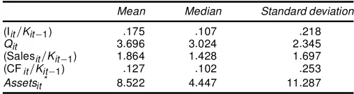
Table 1. Statistics of Regression Variables
Mean Median Standard deviation
(Iit=Kit¡1) :175 :107 :218
Qit 3:696 3:024 2:345
(Salesit=Kit¡1) 1:864 1:428 1:697
(CFit=Kit¡1) :127 :102 :253
Assetsit* 8:522 4:447 11:287
* In billions of new Taiwan dollars at the 1991 price level. One new Taiwan dollar in 1991 exchanges for 1/25.75$ U.S. dollars.
2000), two main factors cause rms to have different levels of investment in imperfect capital markets (holding investment de-mand identical). First, a rm’s investment is higher (or less con-strained) if it has a higher level of internal funds. The cash ow variable is used to capture this effect. Second, a rm’s invest-ment is less constrained if its informational problem is less se-vere. How severe the information problem is may depend on the rm’s intrinsic characteristics, which may or may not be observable to economists. An oft-used proxy is the asset size (Gertler and Gilchrist 1994; Carpenter et al. 1994; Gilchrist and Himmelberg 1995). Firms with larger assets may have better means of providing collateral to mitigate the information prob-lem. For a given industry, larger rms also tend to be older and more mature, so that the market usually has better access to, and assessment of, the rm’s information.
The foregoing model has the unobservable rm and time ef-fects (fi,¿t) inXit. Also considered is the alternative of exclud-ingfiand¿tfromXitand putting them instead inZit, the func-tion of inefciency. This specicafunc-tion has a random-effects im-plication onfi and¿t, in the sense that they are in the model’s composite error and are thus uncorrelated withXitby construc-tion. (Havingftand¿tin bothXitandZitrequires a maximum likelihood estimation of nearly 400 parameters, which exerts great numerical difculty and thus is not considered as a practi-cal alternative.) The nonnested hypothesis test of Vuong (1989) is used for this specication test. The test is structured in such a way that a positive test statistic indicates that the model of xed effects in Xit is favored, and a negative statistic favors the alternative. The test results in a positive statistic with a
pvalue equal to .32, indicating a slight preference for the stated model.
Table 1 presents the summary statistics of the regression vari-ables. Note that the average value ofQit appears to be large, possibly due in part to the phenomenon of cross-shareholdings among publicly traded rms in Taiwan, a widely held view in the domestic market. Because the cross-held rms have stakes in one another, this creates misaligned incentives for the mem-ber rms to keep one another’s share prices high.
5. ESTIMATION RESULTS
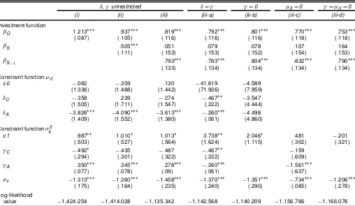
Table 2 gives the results of various model estimations. Estimates of the vast rm and time dummies are not listed. Models (i), (ii), and (iii) are the focus, and they estimate the un-restricted model of (14)–(19). Model (i) includes only the (log of)Qitin the frictionless investment function; under the null of perfect capital markets,Qit is a sufcient statistic. Models (ii)
Table 2. Estimation Results of Eq. (20)
±,°unrestricted ±D° °D0 ¹itD0 °D¹itD0
(i) (ii) (iii) (iii-a) (iii-b) (iii-c) (iii-d)
Investment function
¯Q 1:213¤¤¤ :937¤¤¤ :819¤¤¤ :792¤¤¤ :801¤¤¤ :770¤¤¤ :753¤¤¤ (:087) (:105) (:116) (:116) (:116) (:118) (:118)
¯S :505¤¤¤ :051 :079 :078 :107 :164
(:111) (:153) (:153) (:152) (:154) (:153)
¯S
¡1 :793
¤¤¤ :783¤¤¤ :804¤¤¤ :832¤¤¤ :790¤¤¤
(:133) (:134) (:134) (:134) (:134) Constraint function¹it
c0 ¡:082 ¡:359 :130 ¡41:619 ¡4:589
(1:336) (1:488) (1:442) (71:926) (7:959)
±C ¡:358 :239 ¡:274 ¡:467¤¤ ¡3:547 (1:505) (1:711) (1:547) (:222) (4:444)
±A ¡3:826¤¤¤ ¡4:090¤¤¤ ¡3:613¤¤¤ ¡:260¤¤¤ ¡4:498 (1:409) (1:552) (1:380) (:061) (4:860) Constraint function¾it2
c1 :987¤¤ 1:010¤ 1:013¤ 3:738¤¤ 2:046¤ :481 ¡:201
(:503) (:527) (:564) (1:624) (1:115) (:302) (:321)
°C ¡:492¤ ¡:435 ¡:487 ¡:467¤¤ ¡:159 (:294) (:301) (:322) (:222) (:609)
°A :350¤¤¤ :345¤¤¤ :278¤¤¤ ¡:260¤¤¤ ¡1:561¤¤¤ (:077) (:078) (:09) (:061) (:637)
¾v ¡1:313¤¤¤ ¡1:260¤¤¤ ¡1:458¤¤¤ ¡1:370¤¤¤ ¡1:351¤¤¤ ¡:734¤¤¤ ¡1:206¤¤¤ (:175) (:164) (:235) (:240) (:290) (:085) (:278) Log-likelihood
value ¡1;424:254 ¡1;414:028 ¡1;135:342 ¡1;142:568 ¡1;140:209 ¡1;156:766 ¡1;166:076
NOTE: The xed rm and time effects in the investment function are not listed. Numbers in parentheses are standard errors. Because different numbers of lag variables are used, the number of observations of models (i) and (ii) are different from the rest, and therefore the log likelihood values are not directly comparable. A basic model without the one-sided effect is also estimated. The explanatory variables include theQand the rm and time effects. TheQcoefcient is 1.168, which is signicant at the 1% level, and the corresponding log-likelihood value is¡1,465.909. ¤Signicant at the 10% level.¤¤Signicant at the 5% level.¤¤¤Signicant at the 1% level.
and (iii) also consider the effects of sales ratio variables on the frontier function, as discussed earlier.
Models (iii-a)–(iii-d) build on model (iii) by imposing re-strictions on the modeling of heteroscedasticity. In particular, models (iii-b), (iii-c), and (iii-d) each correspond to an exist-ing model specication in the literature. Model (iii-a) assumes
±D°, requiring variables inZit to have the same coefcients in both the mean and the variance functions of the pretruncated distribution. Model (iii-b) assumes° D0, which corresponds to the specication of Battese and Coelli (1995). Model (iii-c) assumes c0D±C D±AD0, which is the half-normal model with heteroscedastic variances proposed by Caudill, Ford, and Gropper (1995). Model (iii-d) is the original half-normal model proposed by Aigner et al. (1977). Note that this model does not permit exogenous inuences (i.e., cash ow and total asset) to directly explain the one-sided deviation. Results from these models are to be compared with those from model (iii).
As shown in Table 2, theQandSalesratio variables in the in-vestment functions are usually highly signicant, except when a lag of theSalesratio variable is also included, in which case, the contemporaneousSalesratio does not appear to be impor-tant. In ve of the seven models, the elasticity of investment with respect to Q is slightly less than 1; a 1% increase in Q
leads to about .8%–.9% increases in the rate of investment. The effect of sales ratios on investment is also important, exerting about .5–.8 percentage points in terms of elasticity.
As a benchmark, aQmodel without the one-sided deviation effect is also estimated (i.e.,¹itD¾itD0). This is essentially a
linear model withQand xed rm and time effects. The result (not shown in Table 2) has a coefcient ofQequal to 1.168, which is signicant at the 1% level. The adjustedR2 is .472, and the correspondinglog-likelihoodvalue is¡1;465:909. That theQcoefcient is quite close to that of model (i) is not sur-prising, because estimates of the linear model are consistent estimates of the stochastic frontier model. The smaller log-likelihood value, in contrast, reveals the importance of allowing for one-sided deviations in the model. Discussions on this point ensue later in this section.
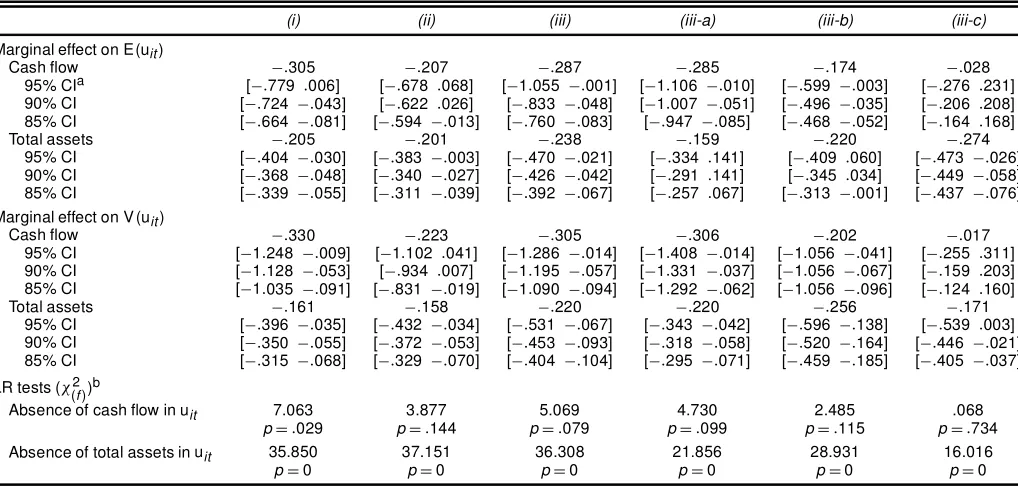
We are interested mainly in the estimates of the nancing constraint effectuit, which is decomposed into the mean func-tion (¹it) and the variance function (¾it2) of its pretruncated dis-tribution. Except in model (iii-d), the mean and variance func-tions are parameterized by cash ow and total asset variables. The reported coefcients are not very informative, however, because they are not the marginal effects due to the model’s nonlinearity. Even thesign of a variable’s latent marginal ef-fect is difcult to tell from the slope coefcients, because the marginal effect depends on estimates in both the ¹it and ¾it2 functions. Therefore, the marginal effects and bootstrap bias-corrected condence intervals are calculated for all of the mod-els except (iii-d). The results, along with some other hypothesis test results, are given in Table 3. Formulas of the marginal ef-fects are provided in the Appendix. The focus is on the signs of the marginal effects.
Table 3 shows that the point estimates of the marginal ef-fects of cash ow and total asset are all negative on both the
Table 3. Marginal Effects and Signicance Testings
(i) (ii) (iii) (iii-a) (iii-b) (iii-c)
Marginal effect on E(uit)
Cash ow ¡:305 ¡:207 ¡:287 ¡:285 ¡:174 ¡:028 95% CIa [¡:779 :006] [¡:678 :068] [¡1:055 ¡:001] [¡1:106 ¡:010] [¡:599 ¡:003] [¡:276 :231] 90% CI [¡:724 ¡:043] [¡:622 :026] [¡:833 ¡:048] [¡1:007 ¡:051] [¡:496 ¡:035] [¡:206 :208] 85% CI [¡:664 ¡:081] [¡:594 ¡:013] [¡:760 ¡:083] [¡:947 ¡:085] [¡:468 ¡:052] [¡:164 :168] Total assets ¡:205 ¡:201 ¡:238 ¡:159 ¡:220 ¡:274
95% CI [¡:404 ¡:030] [¡:383 ¡:003] [¡:470 ¡:021] [¡:334 :141] [¡:409 :060] [¡:473 ¡:026] 90% CI [¡:368 ¡:048] [¡:340 ¡:027] [¡:426 ¡:042] [¡:291 :141] [¡:345 :034] [¡:449 ¡:058] 85% CI [¡:339 ¡:055] [¡:311 ¡:039] [¡:392 ¡:067] [¡:257 :067] [¡:313 ¡:001] [¡:437 ¡:076] Marginal effect on V (uit)
Cash ow ¡:330 ¡:223 ¡:305 ¡:306 ¡:202 ¡:017 95% CI [¡1:248 ¡:009] [¡1:102 :041] [¡1:286 ¡:014] [¡1:408 ¡:014] [¡1:056 ¡:041] [¡:255 :311] 90% CI [¡1:128 ¡:053] [¡:934 :007] [¡1:195 ¡:057] [¡1:331 ¡:037] [¡1:056 ¡:067] [¡:159 :203] 85% CI [¡1:035 ¡:091] [¡:831 ¡:019] [¡1:090 ¡:094] [¡1:292 ¡:062] [¡1:056 ¡:096] [¡:124 :160] Total assets ¡:161 ¡:158 ¡:220 ¡:220 ¡:256 ¡:171
95% CI [¡:396 ¡:035] [¡:432 ¡:034] [¡:531 ¡:067] [¡:343 ¡:042] [¡:596 ¡:138] [¡:539 :003] 90% CI [¡:350 ¡:055] [¡:372 ¡:053] [¡:453 ¡:093] [¡:318 ¡:058] [¡:520 ¡:164] [¡:446 ¡:021] 85% CI [¡:315 ¡:068] [¡:329 ¡:070] [¡:404 ¡:104] [¡:295 ¡:071] [¡:459 ¡:185] [¡:405 ¡:037] LR tests (Â(2
f))b
Absence of cash ow in uit 7.063 3.877 5.069 4.730 2.485 .068
pD:029 pD:144 pD:079 pD:099 pD:115 pD:734 Absence of total assets in uit 35.850 37.151 36.308 21.856 28.931 16.016
pD0 pD0 pD0 pD0 pD0 pD0
aThe bias-corrected condence intervals are bootstrapped from 1,000 replications.
bfis the degree of freedom, which equals 2 for models (i), (ii), (iii), and (iii-a) and 1 for models (iii-b) and (iii-c).
mean and the variance of the nancing constraints. The statisti-cal signicance is revealed by the condence intervals. For the unrestricted models, model (iii)’s negative marginal effects are all signicant at the 5% level, model (i)’s are signicant at the 10% level, and model (ii)’s are at least signicant at the 15% level. In general, the total asset’s effects on the mean and the variance are both very robust, and the cash ow’s effects are more robust on the variance than on the mean.
Bearing in mind some of the marginal cases, the negative effects of cash ow on the mean and variance are of particu-lar interest. The results indicate that in general, acquiring addi-tional cash not only is likely to reduce levels of nancing con-straints, but also decreases the uncertainty of the constraints. The latter effect tends to be more signicant than the former according to the condence intervals. This is the rst study in the literature that documents the cash ow’s second-order ef-fect on the nancing constraint. Unlike the rst-order efef-fect of increasing the level of investment, this second-order effect can-not be explained by the cash ow’s expectation factor. This pro-vides appealing evidence for the nancing constraint hypothe-sis. Similarly, the negative marginal effects of assets state that the level and variance of nancing constraints are smaller for larger rms.
The signicance of the cash ow and total asset variables in the inefciency function was also evaluated. Unlike the con-dence interval analysis, this tests the variable’s overall signif-icance on nancing constraintuit, irrespective of whether the effect is on the mean or on the variance. The null hypothesis is that the variable has no effect on uit. A generalized likeli-hood ratio (LR) test, dened as ¡2[L.H0/¡L.H1/], is used
for this purpose, where L.H0/ and L.H1/ are values of the
log-likelihood functions under the null and the alternative hy-potheses. The statistic has an asymptotic chi-squared distrib-ution with the degrees of freedom equal to the number of
re-strictions. The results are given in the lower panel of Table 3. For the cash ow ratio variable, the worst case is model (iii-c), for which the variable has little statistical justication. As dis-cussed later, however, restrictions imposed on model (iii-c) are overwhelmingly rejected, suggesting that model (iii-c) is mis-specied. For the other ve cases, three of them havepvalues below .10. For the total asset variable, thepvalues are all be-low .01.
All of the foregoing discussions are based on the presumption that the one-sided effect ofuitis signicant in the model, which is a testable hypothesis. Ifuitis not signicant, then it should be dropped from (15), and the model reduces to a neoclassical one with classical disturbances. Furthermore, given the maintained hypothesis thatuit captures nancing constraints, the test ofuit is also a test of whether the nancing constraint is a statistically important phenomenon in explaining the investment behavior. Again, a LR test is used. The model under the null of no effect fromuit is composed of (14)–(16) with nouit in (15), which can be estimated by the traditional panel data method, such as the least squares dummy variable estimator. Because the null hypothesis implies that the variance ofuit is 0, which is on the boundary of the admissible parameter space, the correct asymp-totic of the LR statistic is a mixture of chi-squared distribu-tions (Coelli 1995). Following Coelli and Battese (1996), crit-ical values of the mixed chi-squared distribution are obtained from table 1 of Kodde and Palm (1986). The degrees of free-dom of this statistic equals the number of parameters used to parameterize the distribution ofuit. For models (i)–(iii-a), this number is 6, which has a critical value of 16.074 at the 1% signicance level. For model (iii-b), the number is 4, and the critical value is 12.483. For model (iii-c), the number is 3, and the critical value is 10.501. For model (iii-d), the number is 1, and the critical value is 5.412. The LR test results in the sta-tistics equal to 83.311, 77.633, 86.114, 71.662, 76.381, 43.266,
and 24.646 for models (i)–(iii-d). The null hypotheses of no ef-fect from uit and, equivalently, no nancing constraint effect on investment behavior, are convincingly rejected for all of the models.
Finally, LR tests are performed for four separate hypothe-ses: ±D°, ° D0, ¹it D0, and ° D¹it D0, which are the restrictions on models (iii-a)–(iii-d). On the one hand, these test the validity of the restrictions. On the other hand, they amount to testing whether the cash ow and total asset variables are important for ¹it and¾it2. The null hypothesis is that the re-striction is valid, and the alternative is the unrestrictive spec-ication of model (iii). The tests result in p values equal to
:001,:008, 0, and 0; therefore, the hypotheses are decisively rejected. This had two implications. In terms of model speci-cations, an unrestrictive, exible model on heteroscedasticity is preferred over the four alternatives. In terms of nancing con-straint effects, the cash ow and total asset variables appear to be important for each and both of¹itand¾it2of the pretruncated distribution.
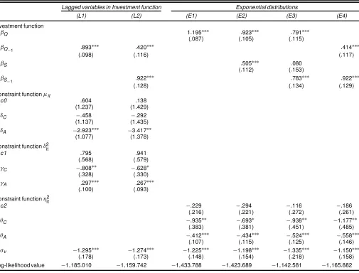
5.1 Alternative Model Specications
This section examines the possibility that the estimated re-sults may be sensitive to different model specications. In par-ticular, two types of alternative model specications are con-sidered. For the rst type, only lagged variables ofQandSales
are included in the investment function. Had there been seri-ous endogeneity problems among the contemporaneseri-ous vari-ables of the investment,Q, andSales, then the lagged variable approach may have been preferred. Whether this modication has any signicant impact on the estimation results is investi-gated.
For the second type of alternative specication, it is as-sumed that the one-sided nancing constraint effect, uit, fol-lows an exponential distribution. Together with half-normal and truncated-normaldistributionsalready used in the models of Ta-ble 2, the exponential is one of the most often assumed distrib-utions in a stochastic frontier analysis. In terms of a prior, note that Kumbhakar and Lovell (2000, p. 90) provided evidence that alternative distributions have nonconsequential effects on the stochastic frontier analysis; whether this holds true in the case herein will be investigated.
The single parameter of an exponential distribution is de-noted by ´ (´ >0). Parallel to the cases of truncated- and half-normal distributions,´is parameterized as a function of observation-specic factors by ´it2Dexp.c2CZitµ /. The log-likelihood function of observationyit is (e.g., Kumbhakar and Lovell 2000)
ln[f.yit/]D ¡ln.´it/Cln
µ
8
³
¡yit¡Xit¯
¾v
¡¾v
´it
´¶
Cyit¡Xit¯
´it
C ¾
2
v
2´it2: (25)
The estimation results are given in Table 4. Models (L1) and (L2) are cases with lagged variables in the investment func-tion. As is shown, estimates in the¹itand¾it2functions are in line with those in Table 2. The marginal effect analysis (not shown) also paints a very similar (if not better) picture; all of
the marginal effects of cash ow and total assets on the mean and the variance of uit are signicantly negative at the 5% level.
Models (E1)–(E4) are cases with exponential distributions. Note that in the case of exponential distributions, the mean and the variance ofuitare´it and´it2. Therefore, signs of the mar-ginal effects need not be recalculated. Again, the negative and signicant marginal effects are consistent with the results of previous models.
It is also of interest to see whether rankings of the obser-vation-specic IEI are sensitive to model specications. The IEI is calculated according to (24), and it quantitatively mea-sures the extent to which nancing constraints affect the rate of investment. This issue is particularly relevant to the analysis in the next section, because the estimated IEI is to be com-pared across rms and over time periods. If rankings of the IEI vary substantially in different models, then the results of the comparisons will be sensitive to the choice of models. To this end, the Spearman rank correlation coefcients between the IEI from the models of Table 4 and from the unrestricted models of Table 2 are calculated. The results are given in Ta-ble 5. As shown, there is high agreement between the rankings from different models, with most of the correlation coefcients well above .90. Note that model (E4) has both of the alternative specications; it uses lagged variables in the investment func-tion and adopts the exponential distribufunc-tion. Even for this case, the correlation coefcients with the compared models are no lower than .88.
The foregoing evidence ensures that results of this study’s analysis are not likely to be signicantly altered if different model specications were to be adopted.
6. POSTESTIMATION ANALYSIS
This section uses the estimated IEI in two different analyses. In the rst analysis, the IEI is used to investigate the validity of some of the sorting criteria used in the literature. In the sec-ond analysis, the IEI is used to evaluate the effects of nancial liberalization in Taiwan during the sample period. The results can be inferred to provide additional evidence of the nancing constraint hypothesis.
The analyses are based on the estimated IEI of model (ii). It can be shown that model (ii) is statistically preferable to model (i) from a LR test. It also retains one more year of data than model (iii), because the latter uses an additional lag variable. The conclusions would change little if the IEI from either model (i) or (iii) were used. Indeed, the IEI from the three models are very close; the Spearman rank correlation coefcients between the three IEIs are .991 for models (i) and (ii), .955 for models (ii) and (iii), and .964 for models (i) and (iii). Models (iii-a)– (iii-d) are not considered, because, as shown previously, the simplifying assumptions on heteroscedasticity used in these models are rejected by the data.
Figure 1 plots the frequency distribution of the IEI. The dis-tribution is skewed to the right with the mean equal to .606 and the standard deviation equal to .190. The mode of the distribu-tion is around .7–.8, indicating a loss of 20%–30% of the rate of investment due to nancing constraints.
Table 4. Results of Alternative Model Specications
Lagged variables in Investment function Exponential distributions
(L1) (L2) (E1) (E2) (E3) (E4)
Investment function
¯Q 1:195¤¤¤ :923¤¤¤ :791¤¤¤
(:087) (:105) (:115)
¯Q
¡1 :893
¤¤¤ :420¤¤¤ :414¤¤¤
(:098) (:116) (:117)
¯S :505¤¤¤ :080
(:112) (:153)
¯S
¡1 :922
¤¤¤ :783¤¤¤ :922¤¤¤
(:128) (:134) (:129) Constraint function¹it
c0 :604 :138
(1:237) (1:429)
±C ¡:458 ¡:292
(1:137) (1:435)
±A ¡2:923¤¤¤ ¡3:417¤¤ (1:077) (1:378) Constraint function±2
it
c1 :795 :941
(:568) (:579)
°C ¡:808¤¤ ¡:628¤ (:328) (:330)
°A :297¤¤¤ :267¤¤¤ (:100) (:093) Constraint function´2
it
c2 ¡:229 ¡:294 ¡:116 ¡:186
(:216) (:221) (:272) (:261)
µC ¡:935¤¤ ¡:693¤ ¡:938¤¤ ¡1:177¤¤
(:383) (:381) (:451) (:485)
µA ¡:412¤¤¤ ¡:434¤¤¤ ¡:524¤¤¤ ¡:558¤¤¤ (:107) (:115) (:125) (:146)
¾v ¡1:295¤¤¤ ¡1:274¤¤¤ ¡1:225¤¤¤ ¡1:198¤¤¤ ¡1:335¤¤¤ ¡1:150¤¤¤ (:178) (:173) (:148) (:154) (:218) (:158) Log-likelihood value ¡1;185:010 ¡1;159:742 ¡1;433:788 ¡1;423:689 ¡1;142:581 ¡1;165:882
NOTE: Models (L1) and (L2) estimate (20), and models (E1)–(E4) estimate (25); see also the footnotes of Table 2.
6.1 Investment Efciency Index by Various Sorting Criteria
As discussed in Section 1, the literature often chooses a sin-gle criterion, such as the asset size, and then picks a critical value of the criterion to separate samples into groups believed to have different characterizations of nancing constraints. The evidence of nancing constraints is then inferred from the com-parisons of cash ow coefcients across the groups.
Implicitly assumed in this approach, however, is that the severity of the nancing constraint problem is signicantly and monotonically related to the sorting criterion. This is necessary
Table 5. Spearman Rank Correlation Coefcients
Models of Table 4
(L1) (L2) (E1) (E2) (E3) (E4)
Unrestricted models of Table 2
(i) .928 .909 .980 .969 .936 .886 (ii) .922 .918 .972 .979 .945 .895 (iii) .944 .971 .935 .942 .981 .947
NOTE: The Spearman rank correlation coefcients between the estimated nancing constraint effects (uitO ) from different models.
so that no matter how the critical value is chosen to separate the samples, one of the two groups would be consistently more nancially constrained than the other. If, however, the relation-ship between the nancing constraint and the sorting criterion
Figure 1. The Distribution of IEI.
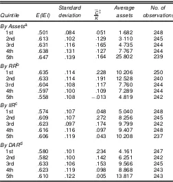
Table 6. Investment Efciency Index by Various Sorting Criteria: The Average Statistics
Standard Average No. of
Quintile E(IEI) deviation SC
K
‡
assets observations
By Assetsa
1st .501 .084 :051 1:682 248 2nd .613 .102 :129 3:110 245 3rd .631 .116 :165 4:735 244 4th .638 .131 :127 7:767 244 5th .647 .139 :164 25:802 239
By RRb
1st .635 .114 :228 10:206 250 2nd .633 .114 :191 12:528 240 3rd .604 .108 :117 7:760 244 4th .597 .100 :109 7:289 244 5th .558 .108 ¡:013 4:819 242
By IIRc
1st .574 .107 :048 5:040 248 2nd .609 .107 :272 8:256 245 3rd .623 .097 :174 9:799 242 4th .616 .116 :097 9:407 248 5th .606 .119 :043 10:208 237
By DARd
1st .580 .101 :234 4:161 247 2nd .582 .100 :142 6:251 242 3rd .633 .106 :153 9:566 245 4th .623 .119 :098 8:868 243 5th .610 .122 :005 13:817 243
‡Average cash ow ratios.
a Total assets, in billions of new Taiwan dollars at the 1991 price level. b Retention ratio: 100£(net income after dividend)/(net income).
c Interest coverage ratio: 100£(interest expenses)/(net incomeC:75£interest expenses). d Debt-to-asset ratio: 100£(total liability)/(asset).
is inconsequential or nonmonotonic, then a chosen cutoff point is not guaranteed to separate samples into groups that have dis-tinct nancing constraint characteristics.
In this section the Taiwanese data are used to investigate the validity of some of the sorting criteria used in the literature. The approach is simple. Because IEI is a measure of nancing constraints, the samples are simply classied into groups by the criterion, and then the sample mean of IEI of each groups is calculated. Comparing the averaged IEI and the associated sta-tistics across the groups reveals whether the differences are sig-nicant and whether the relationships are monotonic. Because of the different data sources, the results are not a direct assess-ment of the current literature, for which the bulk of studies are based on U.S. data.
When sorting the samples, rst the criterion’s average values for each rm are calculated, and then the samples are classied into ve quintiles with roughly equal numbers of rms. Because rms may have different numbers of observations (unbalanced panel), the numbers of observations in the quintiles are not ex-actly the same. Table 6 lists the results with some related statis-tics. Table 6 presents the standard deviationsof the sample aver-age gures, which are bootstrappedfrom 1,000 replications.For an easier presentation, the numbers are plotted and the graphs presented in Figure 2.
6.1.1 Asset Sizes. The rst panel of Table 6 uses the as-set size as the sorting criterion (e.g., Gertler and Gilchrist 1994; Carpenter et al. 1994; Gilchrist and Himmelberg 1995). Larger rms are assumed to be less likely to face obstacles in the capi-tal market, because they tend to be older and more mature, and also to have better market recognition. Larger assets may also
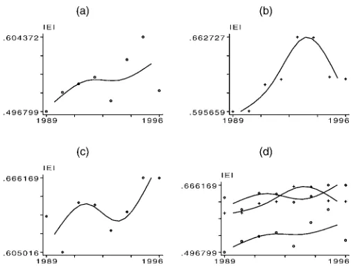
Figure 2. The Monotonicity of Various Sorting Criteria: (a) Size Quan-tiles; (b) Retention Ratio QuanQuan-tiles; (c) Interest Income Ratio QuanQuan-tiles; (d) Debt Asset Ratio Quantiles. The graphs plot the IEI against quantiles of the sorting criteria based on the numbers in Table 6. The literature’s presumption is that asset sizes should be positively related to the IEI, whereas all of the other three criteria should be negatively related to the IEI.
enable them to provide collateral to mitigate information prob-lems.
The result shows that the IEI is monotonically related to the size, increasing from .501 for rms in the rst quintile to .647 for rms in the fth quintile. This difference (.146) ap-pears to be signicantly different from 0; the bootstrapped 90% condence interval, based on 1,000 replications, is between .014 and .366. The monotonic relationship can also be easily seen from the rst graph in Figure 2(a). This conrms the nd-ings of many related studies that larger rms tend to have higher investment efciency.
Note that even for the most investment-efcient group (the rst quintile), the average investment efciency is only .647. This means that the group’s average investment rate is about 64.7% of that of the hypothetically best practice rm. The de-ciency is apparent and indicates the wide-spread nancing con-straint problem among all classes of rms.
6.1.2 Retention Ratios. The second panel of Table 6 uses the retention ratio as the sorting criterion (e.g., Fazzari, Hubbard, and Petersen 1988; Bond and Meghir 1994). A high retention ratio is likely to result from high opportunity costs of dividends, and it can be inferred that rms with higher opportu-nity costs of dividends are those facing more serious nancing constraints.
The average IEI in the rst quintile is .635, and the num-ber declines monotonically over the quintiles to the lowest of .558; the graph in Figure 2 shows the monotonicity. The boot-strapped 95% condence interval of the difference.¡:076/is from¡:163 to¡:008. This result is in accordance with the pre-diction that high retention ratios are associated with nancing constraint problems.
An oft-raised question, however, is whether the discrimina-tory power of the ratio results from its close approximation to rms’ asset sizes. This concern seems to be partially supported by Table 6; the fth column shows that higher retention rms
tend to be smaller ones, although an exception in the rst two quantiles is also noted.
We further investigate this issue by estimating model (ii) with the retention ratio variable added into the functions of¹it and
¾it2. The estimated coefcients of the variable are:002 and:004 in the functions of¹itand¾it2, both of which are statistically in-signicant. An LR test of the joint signicance of the ratio vari-able yields an chi-squared statistic equal to :403, and the null hypothesis of no effect cannot be rejected. Therefore, on con-trolling for the size effect, it is found retention ratios do not pro-vide additional information in distinguishing constrained and unconstrained rms in the data.
6.1.3 Interest-to-Income Ratios. The third panel of Ta-ble 6 classies samples by interest-to-income ratios (e.g., Whited 1992). The ratio indicates the likelihood of a rm in nancial distress. If a rm had sufcient internal nance, then it would not have a great need to borrow.
Unlike in the previous cases, the ratio here does not seem to be monotonically related to the average IEI. Instead, a look at the graph in Figure 2 suggests a concave relationship, with the rst quintile having the lowest value of investment efciency (.574, probably owing to underutilized borrowing capacities) and the third quintile having the highest (.623). Based on these point estimates, moderate ratios are favored in terms of invest-ment efciency. For statistical signicance, the difference be-tween the rst and the third quintiles is marginally signicant at the 15% level (again from bootstrapping), but the difference between the third and the fth quintiles is not appreciable at reasonable signicant levels.
What does this result imply? As noted, the literature hy-pothesizes that rms with higher interest-to-income ratios have greater problems nancing investment, implying a negatively sloped line in the IEI to the interest-to-income ratio plot. The results herein, however, show that the empirical line is likely to bepositivelysloped when the ratio is relatively low and that the variable may not be able to discern degrees of nancing constraints when the ratio is relatively high. This makes the interest-to-income ratio an unappealing sorting criterion when applied to the Taiwanese data.
6.1.4 Debt-to-Asset Ratios. The fourth panel of Table 6 uses the debt-to-asset ratio as the sorting criterion (e.g., Whited 1992). This ratio is a measure of current demand for borrowing relative to the rm’s debt capacity.
Similar to the interest-to-income ratio, the average IEI is at the highest, .633, in the middle quintile, indicating a possible concave relationship between the criterion and the degree of nancing constraint. Again, bootstrapped condence intervals show that the difference is signicant at the 15% level between the rst and the third quintiles, but statistically insignicant be-tween the third and the fth quintiles. The ndings are similar to those of the previous case. The literature has presumed a neg-ative relationship between IEI and debt-to-asset ratios, but the results indicate that the relationship is either positive (quintiles 1–3) or inconsequential (quintiles 3–5).
The foregoing analysis points to asset sizes and retention ra-tios as better sorting criteria for Taiwanese data, although it also shows that retention ratios obtain the discriminatory power mainly from their associations with asset sizes. The other crite-ria (the interest-to-income ratio and the debt-to-asset ratio) do
not seem to have the predicated relationships with investment efciency.
This section concludes with a few more regressions of the augmented linear investment model as used by Carpenter et al. (1994). As we stated in Section 1, at least two different aspects of this approach have drawn criticism. One aspect is that con-cerning the fundamentals of the unstructured linear models, and the other is the justication of using various sorting criterions to split samples. In light of the results of the better sorting cri-terions, assessing the linear model’s ability to capture nanc-ing constraint effects after the issue of sortnanc-ing can be set aside would be desirable.
The samples are split into three groups, based on asset size and retention ratios. A standard xed-effect panel data model is estimated for each of the groups. This model is
ln corresponding coefcient vector. The error termvitis symmet-rically distributed with mean 0. According to Carpenter et al. (1994), the cash ow coefcients should indicate the severity of nancing constraints. The estimation results are given in Ta-ble 7.
For samples classied by rm sizes, Table 7 shows that larger rms’ investment tends to respond more strongly to cash ows. This result matches the ndings of Kaplan and Zingales (1997, 2000), and it is the opposite of Carpenter et al.’s hypothesis. For samples classied by retention ratios, the results also do not support Carpenter et al.’s hypothesis.
Linear investment models with augmented cash ows are not adequate to capture the effects of nancing constraints on Tai-wanese rms. The stochastic frontier approach gives evidence of nancing constraints on smaller rms and on high–retention ratio rms; the same cannot be obtained using the linear regres-sion approach.
6.2 Effects of Financial Liberalization
As described in Section 1, Taiwan’s nancial markets un-derwent liberalization reforms in the sample period. The the-ory predicts that the process should help release nancing con-straints for most of the rms, and for underprivileged rms in particular. Table 8 shows the average IEI across time for all of the rms, as well as for three groups of rms classied by asset sizes. The classication is based on the 33rd and 66th quantiles of the average size distribution.
The IEI of the total samples is the lowest in 1990 (.578); it rises in the next 2 years before experiences a small setback in 1993. The number is up again in 1994 and 1995, reaching the highest level of .631 in the sample period. This is to say that the loss of the rate of investment for an average rm was reduced by 5.3 percentage points from 1990 to 1995. This period chronicles
Table 7. Linear Investment Model of (26)
By asset sizes By retention ratios
Small Median Large Small Median Large
¯Q :729 :845 :71 1:335 :154 :776
(:260)¤¤¤ (:231)¤¤¤ (:249)¤¤¤ (:226)¤¤¤ (:246) (:240)¤¤¤
¯S :343 :108 ¡:223 ¡:370 :226 :306
(¡:314) (¡:293) (¡:315) (:320) (:305) (:288)
¯S
¡1 :538 :709 1:275 :637 1:109 :555
(:284)¤ (:244)¤¤¤ (:273)¤¤¤ (:296)¤¤ (:275)¤¤¤ (:253)¤¤
¯C :087 ¡:262 :431 :251 :309 ¡:102
(¡:285) (¡:277) (¡:268) (:260) (:255) (:361)
¯C
¡1 ¡:487 :102 :723 ¡:401 :596 ¡:131
(¡:313) (¡:304) (:338)¤¤ (:296) (:340)¤ (:326) Sum of cash ow ¡:400 ¡:160 1:153 ¡:150 :905 ¡:233
coefcients (:439) (:443) (:514)¤¤ (:415) (:512) (:501)
S
R2 :181 :252 :158 :107 :232 :163
Average criterion 2.056 (bill.) 4:846 15:909 :429 :874 :992 No. of observations 338 342 334 341 336 337
NOTE: The xed rm and time effects are not listed. Numbers in parentheses are standard errors. Also see the footnotes in Table 2.
some important nancial reforms in the Taiwanese markets, as discussed in Section 1. The average IEI dropped substantially, however, to .603 in 1996, the last year in the sample. This set-back is likely to be triggered by the political and military intim-idations of the Beijing government toward Taiwan in late 1995 and early 1996. The tension began from then-Taiwan President Lee Teng-Hui’s visit to the United States in June 1995, and es-calated with Beijing’s missile tests off the coast of Taiwan in March 1996, around the day of the rst direct presidential elec-tion in Taiwan. Beijing’s military threat led the United States to send forces into the region. Undoubtedly, this event had ad-versely affected investors’ and nanciers’ condence.
The average IEI for rms of different sizes are given in the third, fourth, and fth columns of Table 8, and these numbers are plotted in Figure 3 for easier presentation. The lines in Fig-ure 3 are drawn through the medians of pairs of the data points, thus representing biannual trends of IEI.
The average IEI of the small rms was always lower than those of median- and large-sized rms. For the small rms, the number was at its lowest (.497) in 1989 and reached its highest level of .604 in 1995, which is an increase of about 10 percent-age points in term of investment efciency. Median-sized rms also showed continuousefciency gains in the early 1990s, with
Table 8. The Effects of Financial Liberalization on Firms of Different Sizes: A Comparison of Investment Efciency Index Across Time
All Small Medium Large No. of
Year rms rms rms rms observations
1989 .580 .497 .596 .635 101 1990 .578 .525 .596 .605 115 1991 .604 .537 .620 .646 131 1992 .606 .546 .625 .644 148 1993 .598 .512 .663 .623 173 1994 .622 .572 .662 .638 184 1995 .631 .604 .627 .666 184 1996 .603 .527 .625 .666 184 No. of 1220 412 402 406
observations
NOTE: Samples are classied by the average asset sizes at the 33rd and 66th quantiles. They show that the IEI of small rms has increased more signicantly over the period.
a gain of about 6.7 percentage points from the lowest to the highest. The group of large rms also had a maximum gain of 6.1 percentage points in the IEI in this period.
The combined graph in Figure 3(d) shows interesting com-parisons. The lines of pairwise medians indicate an increases in the biannual trend of IEI for small rms in the sample pe-riod. The trend was also in the rise for medium-sized rms from 1990 to 1994, but the same cannot be said for the group of large rms. Indeed, the increasing trend of small rms has such an effect that the difference between large rms’ and small rms’ IEI narrowed from .138 in 1989 to .062 in 1995, although the number widened again in 1996.
The evidence presented in this section is favorable to the -nancing constraint hypothesis. In particular, the nding of the disproportionalgain for smaller rms in the nancial liberaliza-tion process is new and strong evidence of nancing constraint that has not yet been documented in the literature.
Figure 3. Small Firms Gained More From Financial Liberalization. The biannual trend lines are drawn through the medians of pairs of the data points. (a) Small-size rms; (b) medium-size rms; (c) large-size rms; (d) all rms.
7. CONCLUSION
This article has shown that investment of nancing-cons-trained rms can be modeled as a one-sided deviation from a frictionless model. By imposing the distribution assumption on the constraint, the effect of nancing constraints can be identi-ed and quantiidenti-ed and some of the shortcomings of the regres-sion method can be avoided.
The results are very encouraging. For cash ow, not only is it likely to promote the rate of investment in an environment of nancing constraints, but it also has a strong effect on reducing the variance of nancing constraints. This second-order effect is appealing evidence for the nancing constraint hypothesis, because the oft-alleged role of cash’s investment expectation cannot be applied here to explain this result.
This article has also investigated some of the oft-used criteria in the literature for splitting samples into a priori constrained and unconstrained groups. Of particular interest was whether the criteria are signicantly and monotonically related to the degree of nancing constraints. For the Taiwanese data, it was found that the asset size and the retention ratio are better cri-teria, and that the interest coverage ratio and the debt-to-asset ratio appear to be more problematic.
Comparisons of the investment efciency index across time for different groups of rms are also revealing. Using Taiwan’s nancial liberalization as a natural experiment, it was shown that the investment efciency improved for a typical rm dur-ing the process, and that the improvement was particularly sig-nicant for rms of smaller asset sizes.
ACKNOWLEDGMENTS
The author thanks Cliff Huang and Peter Schmidt for helpful discussions and Fung-Mey Huang, Ming Liu, James Tybout, and two referees for valuable comments. Financial support was provided by the National Science Council of Taiwan grant 89-2415-H-001-064.
APPENDIX: Replacement Cost of Capital and Marginal Effects
A.1 Replacement Cost of Capital
The method of Lewellen and Badrinath (1997) is used to un-cover the vintage structure of period t’s net capital stock. It is sketched as follows (see Lewellen and Badrinath 1997) for more details. First, periodt’s gross capital stock is obtained by adding up period t’s accumulated depreciation of capital and the net capital stock. Because the gross capital stock is the ac-cumulation of past periods’ gross capital investment, the gross capital investment are added upbackwardin time starting from periodtuntil the sum of the investment equals the gross capital stock of periodt. Equivalence occurring at periodt¡N im-plies that periodt’s capital stock is accumulated from period
t¡N. With assumed depreciation rates, the current value of each vintage of periodt’s net capital stock can then be calcu-lated.
The rms’ periodic reports on revaluations of selected assets are also used to aid calculation of the market value of capi-tal. In particular, because local regulation permits asset revalu-ations only when the price level has increased by 25% relative
to the purchasing year, this information is used in the interpo-lation of asset prices. Also, because land prices in Taiwan have increased disproportionally relative to other asset prices in the past decades, the land value is calculated separately from other xed assets.
A.2 Marginal Effects onE(uit) andV(uit)
For models (i), (ii), and (iii), the unconditional mean and variance ofuitare
E.uit/D¾it vector in (18) and (19), can be derived by taking the derivatives of the foregoing functions with respect toZ[k]. Tedious manip-ulations lead to efcient vectors. The formula is evaluated at every observation, and the sample average is reported. The marginal effects for models (iii-a)–(iii-c) can be derived similarly.
It is interesting to note that in (A.3) a nonparameterized¾2
would imply a monotonic effect ofZ[k] onE.uit/. To see this, note that°[k]D0 if¾2is constant, and that the function in the big square bracket of the remaining term is positive (more precisely, between 0 and 1, as shown in the literature of lim-ited dependent variables). Thus the marginal effect takes the sign of±[k], which is xed for all values ofZ[k]. This in turn implies thatE.uit/is monotonic in Z[k]. On the other hand, nonmonotonic relationships are accommodated if¾2 is para-meterized byZand°[k] is not 0.
[Received April 2001. Revised October 2001.]