Full Terms & Conditions of access and use can be found at
http://www.tandfonline.com/action/journalInformation?journalCode=ubes20
Download by: [Universitas Maritim Raja Ali Haji] Date: 11 January 2016, At: 22:57
Journal of Business & Economic Statistics
ISSN: 0735-0015 (Print) 1537-2707 (Online) Journal homepage: http://www.tandfonline.com/loi/ubes20
Identification of Expected Outcomes in a Data
Error Mixing Model With Multiplicative Mean
Independence
Brent Kreider & John V. Pepper
To cite this article: Brent Kreider & John V. Pepper (2011) Identification of Expected Outcomes
in a Data Error Mixing Model With Multiplicative Mean Independence, Journal of Business & Economic Statistics, 29:1, 49-60, DOI: 10.1198/jbes.2009.07223
To link to this article: http://dx.doi.org/10.1198/jbes.2009.07223
Published online: 01 Jan 2012.
Submit your article to this journal
Article views: 63
Identification of Expected Outcomes in a Data
Error Mixing Model With Multiplicative
Mean Independence
Brent KREIDER
Department of Economics, Iowa State University, Ames, IA 50011-1070 (bkreider@iastate.edu)
John V. PEPPER
Department of Economics, University of Virginia, Charlottesville, VA 22904-4182 (jvpepper@virginia.edu)
We consider the problem of identifying a mean outcome in corrupt sampling where the observed outcome is drawn from a mixture of the distribution of interest and another distribution. Relaxing the contaminated sampling assumption that the outcome is statistically independent of the mixing process, we assess the identifying power of an assumption that the conditional means of the distributions differ by a factor of proportionality. For binary outcomes, we consider the special case that all draws from the alternative distribution are erroneous. We illustrate how these models can inform researchers about illicit drug use in the presence of reporting errors.
KEY WORDS: Contaminated sampling; Corrupt sampling; Measurement error; Nonparametric bounds; Partial identification.
1. INTRODUCTION
Empirical analyses have long struggled with how to draw credible inferences in light of data errors that arise from a va-riety of sources and are often known to be extensive. In the 2001 Current Population Survey, for example, the wages of nearly a third of the workers are imputed (Hirsch and Schu-macher2004) and validation studies consistently reveal large and systematic reporting errors even for variables one might think should be reported accurately (see, e.g., Bound, Brown, and Mathiowetz2001). Credible solutions to these data error problems, however, remain elusive. The assumptions of the nondifferential errors-in-variables models are often untenable (see, e.g., Bound, Brown, and Mathiowetz2001for discussion), and alternative models rely on parametric assumptions that can be difficult to justify in many applications. There is good rea-son, therefore, to consider alternative approaches.
Recently, a growing body of literature conceptualizes the data error problem using a mixture model in which the observed outcome distribution is a mixture of the unobserved distribu-tion of interest,F, and another unobserved distribution,G[see, e.g., Horowitz and Manski1995(HM henceforth); Lambert and Tierney1997; Dominitz and Sherman2004; Mullin2005; Krei-der and Pepper2007,2008]. In this environment, the “contami-nated sampling” model pertains to the case in which data errors are known to be statistically independent of sample realizations from the population of interest. The more general “corrupted sampling” model pertains to the case where nothing is known about the pattern of data errors. Using nonparametric methods, HM derived sharp bounds on parameters ofFunder both cor-rupt and contaminated sampling for the case that the researcher has an upper bound on the fraction of draws that come fromG. In this article, we study what can be inferred about the ex-pected outcome given assumptions about how the mean of F
varies with the mixing process. Specifically, we relax the statis-tical independence assumption embodied in the contamination
model to instead consider the identifying power of mean inde-pendence and, most notably, a variant we call “multiplicative mean independence.” In the latter case, the conditional means are allowed to differ by a known or bounded factor of propor-tionality. Our approach is motivated by the observation that, in practice, corrupt sampling bounds tend to be frustratingly wide given the lack of structure on the measurement error process, while the contamination independence assumption is often un-tenable. For example, income nonresponse is thought to be re-lated to income levels, and the accuracy of reported health sta-tus is thought to be related to true health stasta-tus (e.g., Bound, Brown, and Mathiowetz2001). Likewise, in our empirical ap-plication described in the following, the misreporting of illicit drug use is thought to occur more frequently among users than nonusers. While the independence assumption is unlikely to hold in these examples, it seems reasonable to apply the multi-plicative mean independence model developed in this article.
We begin in Section 2 by studying the identifying power of the multiplicative mean independence model. Applying the contaminated sampling results in HM, we are able to partially identify the expected outcome for any distribution with a finite mean. We then illustrate the partial identification bounds under the important special case of a binary outcome distribution. In Section 3, we further consider the problem of identifying bi-nary outcome distributions under additional restrictions. In this context, researchers using mixture models often assume (some-times implicitly) that all draws fromGare known to be inaccu-rate, as might be the case when mixing arises from response er-ror. This response error mixture model provides a link between
FandGthat is especially informative for binary outcome distri-butions: in this case, realizations fromGreveal precisely what
© 2011American Statistical Association Journal of Business & Economic Statistics
January 2011, Vol. 29, No. 1 DOI:10.1198/jbes.2009.07223
49
the outcome of interest is not. Not surprisingly, imposing this additional assumption has substantial identifying power.
The parts of our analysis that focus on binary variables are related to Molinari (2008) who presented an alternative con-ceptualization of the data error problem for discrete outcome variables. In her “direct misclassification” approach, she fo-cuses on assumptions related to classification error rates in-stead of restrictions on the mixing process. For corrupt and contaminated samples, Molinari derived the same closed-form bounds provided in HM. While she did not consider multiplica-tive mean independence restrictions directly, in principle her computational methods can handle this type of restriction when considering binary outcome distributions. From a practical per-spective, however, it is not clear how one would explicitly map our more general multiplicative mean independence assump-tion into exhaustive restricassump-tions on misclassificaassump-tion probabil-ities. Moreover, we derive closed-form identification regions, tailored to our maintained assumptions, that are not available in her analysis.
In contexts where theory or validation data implies direct re-strictions on misclassification probabilities, Molinari’s frame-work provides a natural method for producing the associated identification regions. Our proposed framework is natural for cases in which the researcher has knowledge about conditional means. For example, it is straightforward in our framework to impose a restriction that the prevalence rate of illicit drug use is higher among inaccurate responders than among accurate re-sponders. The mixing distribution framework is also well suited for studying data problems in which corrupt responses do not necessarily constitute misclassifications. For example, cases in which the data are corrupted with imputations or proxy re-sponses are better handled in a mixing framework that allows for the possibility that observations fromGmay be accurate.
In Section4, we apply these methods to the problem of using self-reported surveys to infer the fraction of the noninstitution-alized population consuming illicit drugs. In this application, we find that a response error model with multiplicative mean independence is easy to motivate and can have substantial iden-tifying power. Finally, we draw conclusions in Section5.
Throughout, we simplify the exposition by leaving implicit any conditioning variables; one can condition our results on any observed covariates. The recent literature on partial identifica-tion considered restricidentifica-tions between covariates and the mixing distributions. In particular, instrumental variable and verifica-tion assumpverifica-tions have been shown to reduce the ambiguity re-sulting from data errors (see Lambert and Tierney1997; Do-minitz and Sherman 2004; Kreider and Pepper 2007, 2008). Layering these assumptions on top of the multiplicative mean independence assumption will serve to narrow the bounds pre-sented in this article.
Finally, since our focus is on identification, we treat identi-fied quantities as known. In the empirical section, we can con-sistently estimate the derived identification bounds by repling population probabilities with their sample analogs. To ac-count for sampling variability, a growing body of literature has developed procedures for drawing inferences in partially iden-tified models (e.g., Imbens and Manski2004; Beresteanu and Molinari2008; Rosen2008; Stoye2009) that can be applied to the bounds derived in Proposition1. Application of these ap-proaches for the response error mixture model in Proposition2,
however, can be complicated because the bounds vary discon-tinuously. Molinari (2008) proposed a method of inference for similar problems that might be useful in this setting. We focus, however, on the question of identification.
2. MULTIPLICATIVE MEAN INDEPENDENCE
In this section, we define and characterize the identifying power of the multiplicative mean independence assumption. In Section2.1, we introduce the notation and the basic question, and then we review some of the relevant findings from HM. In Section2.2, we define the multiplicative independence assump-tion and derive bounds on the mean outcome that apply under this restriction. In Section2.3, we consider the special case of a binary outcome where we can find closed form bounds.
2.1 The Mixture Model and Identification With Contaminated Sampling
To distinguish between the reported and true outcome dis-tributions, letW be the outcome of interest and letZ indicate whether the observed outcome, X, comes from F or G. As-sume that the means ofXandW exist. Our interest is in
learn-ingw≡E(W), but we only observe the outcome distribution
X=WZ+W(1−Z)whereW is the random variable drawn from the alternative distribution,G. An identification problem arises because knowledge ofXalone does not revealE(W).
The mean outcome, however, can be partially identified un-der a variety of different restrictions on the mixing process. A common starting point in this literature is to assume a known lower boundvon the fraction of cases that are drawn from the distribution of interest,F:
Assumption 1.
z≥v, (1)
wherez≡P(Z=1).
This type of restriction is used in the literature on robust sta-tistics (Huber1981) and data errors with binary regressors (see, e.g., Bollinger1996; Frazis and Loewenstein2003). A partic-ular lower bound restriction may be informed by a validation study of a related population or the known fraction of responses that are imputed (see, e.g., HM; Dominitz and Sherman2004; Kreider and Pepper2007,2008).
LetX∈ [kx0,kx1]and, for simplicity, be continuous. Given this restriction, Horowitz and Manski (1995, corollary 4.1) showed that
vE(X|X≤τX(v))+(1−v)kx0
≤w≤vE(X|X> τX(1−v))+(1−v)k1x, (2)
whereτX(·)is the quantile function for the distribution of X. These bounds are easily generalized to allow for noncontin-uous outcome distributions (see Horowitz and Manski 1995 and Dominitz and Sherman2004). Notice that in this conserva-tive “corrupted sampling” environment, identification ofE(W) deteriorates rapidly with the allowed fraction of misclassifica-tions, 1−v.
Prior information can narrow these corrupt sampling bounds. A common assumption known to have identifying power is that
the sampling process is contaminated, in which case the mixing processZis independent of the outcome distribution of interest:
P(W)=P(W|Z). Given Assumption1, Horowitz and Manski
(1995, corollary 4.1) derived sharp bounds on the conditional mean,E(W|Z=1):
E(X|X≤τX(v))≤E(W|Z=1)≤E(X|X> τX(1−v)). (3)
Under contaminated sampling, these bounds also apply to the quantity of interest,E(W), sinceE(W)=E(W|Z=1).
Two features of the contaminated sampling bounds are worth highlighting. First, the contaminated sampling bounds in Equa-tion (3) are weakly narrower than the corrupt sampling bounds in Equation (2). Second, these sharp bounds onE(W)are infor-mative even if the support of the distribution ofXis unbounded. Thus, given Assumption1, we can find meaningful bounds on the conditional expectationE(W|Z=1)for any observed out-come distribution with a finite mean. In the next section, we use this result to derive sharp bounds onE(W)under a generaliza-tion of the contaminated sampling assumpgeneraliza-tion.
2.2 Identification With Multiplicative Mean Independence
Given our interest in the mean outcome,E(W), one obvious way to relax the statistical independence restriction is to con-sider a mean independence restriction thatE(W)=E(W|Z). As we see in Equation (3), this mean independence assumption is sufficient to derive the contaminated sampling bounds onw. In many empirical applications, however, both the statistical inde-pendence and mean indeinde-pendence assumptions may be unten-able. It seems unlikely, for example, that the misreporting of illicit drug use is orthogonal to actual drug use status or that the true income distribution is mean independent of whether re-sponses are imputed or self-reported.
Our notion ofmultiplicative mean independencegeneralizes the mean independence restriction by allowing the two condi-tional means to differ by a factor of proporcondi-tionality. That is, for
z<1:
Assumption 2.
E(W|Z=0)=γE(W|Z=1) (4)
for some known or bounded value ofγ∈ [0,∞).
Under fully accurate reporting,z=1, Assumption2provides no identifying information:E(W)=E(X). In some cases, a par-ticular value ofγ may be informed by a validation study of a related population. Otherwise, one can often rule out values of γ less than 1 or values greater than 1. For example, the use of illicit drugs is thought to be at least as prevalent among inac-curate reporters as among acinac-curate reporters. In this context, a model that imposes the restrictionγ≥1 may be credible when the restrictionγ=1 is untenable.
Proposition 1 provides sharp bounds on the expected out-comeE(W)in this more general setting. We begin by deriving
E(W)as a function ofγ,E(X), and the unobserved probability
z. Using the law of iterated expectations, we see that
E(W)=E(W|Z=1)z+E(W|Z=0)(1−z).
Then, given Assumption2, we have
E(W)=E(W|Z=1)[1+(γ −1)(1−z)]. (5)
Bounds on E(W)follow directly from Equation (5). To see this, suppose the fraction observations drawn from the distri-bution of interestzis known. As we see in Equation (3), HM derived informative bounds on the unknown conditional expec-tation, E(W|Z=1), under Assumption 1. These HM bounds apply whenever the mean of the observed outcome exists, re-gardless of whether the support of the distribution is bounded. If, however, the unobserved random variableWis known to lie within the bounded support, [k0,k1], then Assumption 2
fur-Thus, for a knownz, Equation (6) provides informative bounds onE(W).
Whenzis unknown, bounds onE(W)are found by taking the infimum ofLB(·)and the supremum ofUB(·)over all feasible values ofz. This set of feasible values is restricted directly by Assumption1 and indirectly by Assumption2. Assumption1 rules out all values ofz<vand Assumption2rules out values ofz∈ [0,1)where the associated HM bounds onE(W|Z=1) lie strictly outside[k0
γ,
Thus, z is restricted to exceed vand to satisfy the condition in Equation (7). Notice that ifvdoes not satisfy the condition in Equation (7), then the monotonicity of the HM bounds with respect tozimplies that there are no feasible values ofz<1. In this case,z=1 andE(W)=E(X).
Given these restrictions on feasible values onz, we have:
Proposition 1(Multiplicative mean independence). Suppose Assumptions1and2hold withγ andvknown. Letbe the set
If the conditions in Equation (7) are satisfied, the lower bound simplifies to min{E(X),LB(v)}forγ ≤1 and the upper bound simplifies to max{E(X),UB(v)}forγ ≥1. If the conditions in Equation (7) are not satisfied,E(W)=E(X).
A proof of these closed form results is provided in the Ap-pendix. Notice that closed form results for the upper and lower bounds onE(W)can be found for certainγ, but not in general. In particular, both terms of the upper bound in Equation (6) monotonically decrease withzwhenγ ≥1, and both terms of the lower bound increase with z whenγ ≤1. In these cases, closed form bounds can be found by evaluating Equation (6) at the smallest feasible value ofzsubject to the constraints im-plied by Assumption2. When the two terms move in opposite directions, no closed form result applies for all distributions and allz. Finally, notice that whenγ=1, the Proposition1bounds are identical to the HM contaminated sampling bounds on the expected outcome in Equation (3).
2.3 Illustration: Binary Outcome Distribution
For binary outcomes, where k0=0 and k1=1, the HM
bounds in Equation (3) become (p −min{1 − v,p})/v≤ E(W|Z=1)≤(p−max{p−v,0})/v, where p≡E(X). Ap-plying Proposition1, we find:
Corollary 1. Let W andX be Bernoulli random variables. Then by Proposition1,
min{p,LB(v)} ≤w≤maxp,min{UB(v),p+γ (1−p)}.
A proof is provided in theAppendix. Notice that the lower bound attains the HM corrupt sampling lower bound when γ=0. The upper bound attains the HM corrupt sampling upper bound whenγ=vp(forv≥p).
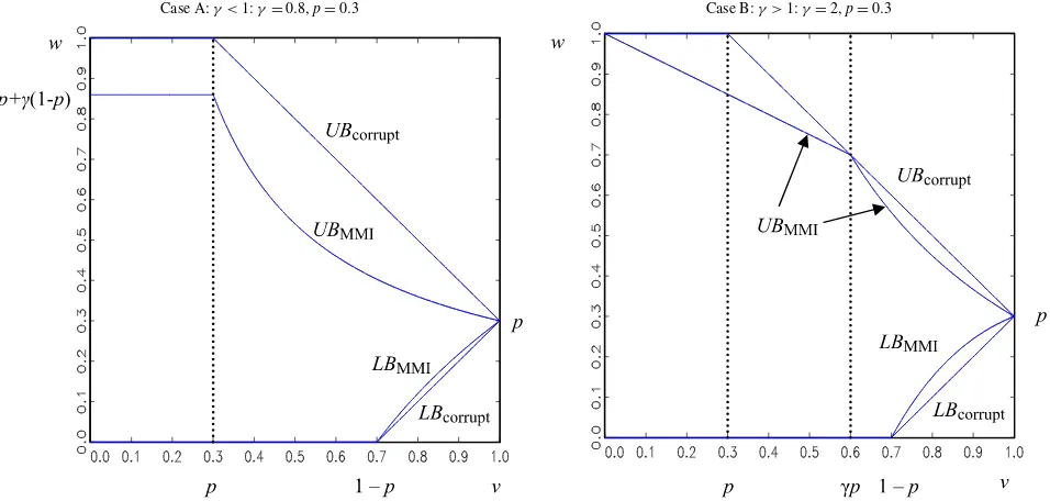
Figure1 illustrates these identification regions under hypo-thetical combinations of {γ ,p}, where the curvesLBMMI and UBMMI trace out the Proposition1 bounds onwas a function ofv. A representative case whenγ <1 is presented in Case A, and a representative case whenγ >1 is presented in Case B. The diagonal lines converging atw=preflect the HM corrupt sampling bounds. For v<1, the Proposition1 bounds are al-ways weakly more informative than the corrupt sampling HM
bounds, and they may even be informative when there is no prior information on the degree of accurate reporting (v=0). Consider, for example, Case A where γ =0.8 and p=0.3. Ifv=0, the outcome distribution must lie within[0,0.86]. In contrast, under corruption the data reveal nothing about the out-come distribution untilvexceeds 0.3. Both the corrupt and con-taminated sampling lower bounds are uninformative unless over 70% of the responses are known to come from the distribution of interest.
3. THE RESPONSE ERROR MIXING MODEL
While realizations fromGare often referred to asdata er-rors(see Horowitz and Manski1995), the mixing model alone does not impose the restriction that each draw fromGis erro-neous. This feature allows for the possibility that draws fromG
come from a proxy that, for some realizations, provides a valid measure of the distribution of interest (e.g., when contamina-tion arises from imputacontamina-tion). For binary outcomes discussed in Section2.3, however, data errors are often conceptualized as a response error with false negative and positive reports. Thus, we also consider the identifying power of the following response error assumption:
Assumption 3.
P(W=X|Z=0)=0. (8)
We refer to Assumption 3 as the response error mixture model in that all draws from the alternative distribution are known to be erroneous. This assumption provides a link be-tweenFandGthat is informative for discrete outcome distri-butions. Realizations fromG reveal what the outcome of in-terest is not. Thus, for a binary outcome, Assumption 3 im-plies that P(W =1|Z =0)=P(X =0|Z =0) so that X = WZ+(1−W)(1−Z).
To derive analytic identification regions when combining As-sumptions1through3, our strategy is to (a) derive the outcome
Case A:γ <1:γ=0.8,p=0.3 Case B:γ >1:γ=2,p=0.3
Figure 1. Multiplicative mean independence (MMI). The online version of this figure is in color.
probability,w, as a function ofγ,p, and the unobserved proba-bilityz; (b) translate restrictions on false positives and false neg-atives into restrictions on possible values ofz; and then (c) iden-tifywextrema over valid candidates ofz.
3.1 The Outcome Distribution and the Accurate Reporting Rate
Using the law of total probability, decompose the observed outcome distribution to consider information embedded in the reported classifications:
p=P(X=1|Z=1)z+P(X=1|Z=0)(1−z).
It follows from Assumptions2and3that
p=P(W=1|Z=1)[(γ+1)z−γ] +(1−z), (9)
so that we can write the prevalence rate among accurate re-porters as
P(W=1|Z=1)= z−(1−p)
(γ+1)z−γ ifz=
γ
γ+1. (10)
Substituting Equation (10) into Equation (5), we can now write the outcome probability as a function of the unknown ac-curate reporting probability,z:
wis identified. In contrast, knowledge ofzandγdoes not iden-tifyw(z)under Assumption2alone [see Equation (6)]. When
z=γγ+1, Equation (9) reveals that p=γ1+1; this outcome is treated as a special case in Proposition2.
Whilewis not identified whenzis unknown, the outcome distribution can be bounded by consideringw(z)over the feasi-ble range ofz. There are two sources of restrictions onz. First, values ofzless thanvare ruled out by Assumption1. Second, given values ofγ andp, restrictions on false positive and false negative classifications constrain the possible values ofz. For
z=γγ+1, use Equation (10) and Assumptions2and3to write the fraction of false positives as
θ+=P(W=0|Z=0)(1−z)=(z−γp)(1−z)
(γ+1)z−γ , (12)
and the fraction of false negatives as
θ−=P(W=1|Z=0)(1−z)=γ[z−(1−p)](1−z)
(γ+1)z−γ . (13)
The fraction of false positives cannot be negative, nor can it exceed the total fraction of positive classifications:θ+∈ [0,p]. Similarly, the fraction of false negatives cannot be negative, nor can it exceed the total fraction of negative classifications:θ−∈ [0,1−p]. These constraints imply the following restrictions on the accurate reporting rate:
Lemma 1. Given Assumptions2and3, the accurate report-ing rate is bounded as follows: Whenγ=0,z≥1−p. When
A proof is provided in theAppendix.
To illustrate the restrictions on the accurate reporting rate,z, consider the case of contaminated sampling where γ=1 and
p=0.3. Based on Assumptions 2 and3 alone, Lemma1 re-veals thatz∈ [0,0.3] ∪ [0.7,1]. A lower bound accurate report-ing rate, v, provides additional information. As noted earlier, studies assessing measurement error in binary variables often assumez>12. In that case, Assumption1rules out any values of
z≤ 12, while Assumptions2and3rule out values between 0.3 and 0.7. Thus, Assumptions1through3imply that at least 70% of the data are correctly classified. The commonplace restric-tion that more than half the data are correctly classified,z>12, can be sharpened—sometimes quite substantially—under this response error mixture model.
3.2 Bounding the Outcome Distribution
Now that we can identify the set of feasible candidates for
z, it remains to identify the possible range ofwfor each feasi-ble value ofz. To do this, we need to characterize the behav-ior of the functionw(z)across different values ofγ andp. In particular, w(z)is weakly concave in(−∞,γγ+1)and convex in(γγ
+1,∞), or vice versa, depending on the valuesγ andp.
Moreover, the local extrema ofw(z), which play a role in defin-ing the bounds, are sensitive to these parameters.
Before presenting the formal results characterizingw(z), it is instructive to visualize the shape of this function across several different parameter values. Figures2and3depict the identifi-cation regions for different values ofγ,p, andv. Figure2 con-siders the special caseγ=1 (pure contaminated sampling) for the valuesp=0.3 andp=0.7. For comparison, we also depict the corrupt and contaminated sampling bounds. The horizon-tal axis now depicts the unknown fraction of draws,z, from the distribution of interest,F. Values ofzlying between the vertical dotted lines are ruled out by Lemma1.
Under the response error model assumption,w(z)traces out the true prevalence rate as a function ofz. Whenz=1, the true prevalence rate equals the reported prevalence rate:w=p. At the other extreme whenz=0, all classifications are inaccurate andw=1−p. Most importantly, notice that the shape of the outcome distribution functionw(z)depends on the fraction of respondents reporting in the affirmative,p. Whenp=0.7(0.3), for example, the outcome distribution decreases (increases) inz
for feasible values ofzoutside[0.3,0.7].
Forγ =1 in Figure 3, it is useful to study the behavior of
w(z)when (1) γ −1 and p− γ+11 have the same sign, and (2) γ −1 and p−γ1
+1 have opposite signs. The latter case
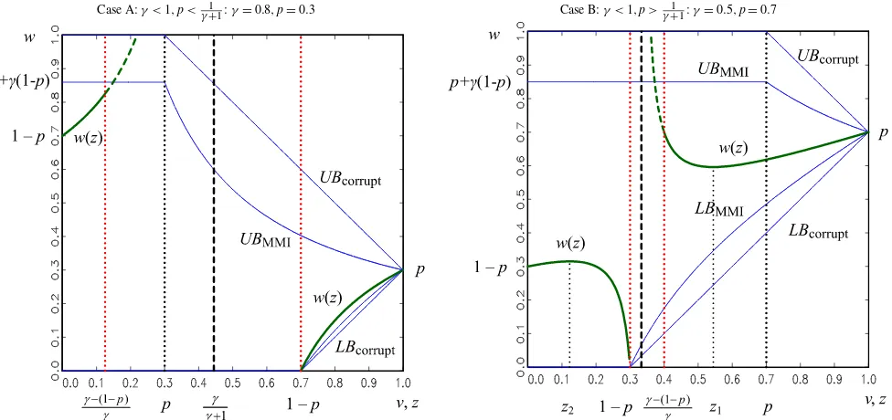
is more complicated because w(z)may exhibit local extrema within z∈(0,1). Figure 3A depicts the first case when both signs are negative: {γ ≤1,p< γ+11}. As in Figure2, w(z)is monotonic inzfor values ofznot ruled out by Lemma1. Specif-ically, the outcome distribution increases over contiguous fea-sible ranges ofz. The figure is analogous for the case that both signs are positive, {γ ≥1,p> γ+11}(not shown), except the outcome distribution decreases in z. When{γ <1,p> γ+11}, as depicted in Figure 3B, w(z)is not monotonic in z, and as such, the bounds may be sensitive to interior extrema. Definez1
andz2as the values ofzthat minimize and maximize,
Case A:γ=1,p=0.3<1/2 Case B:γ=1,p=0.7>1/2
Figure 2. Response error mixture model with mean independence.Note:w(z)traces outwas a function ofz, from which we can find bounds onwfor a givenv. The online version of this figure is in color.
tively, the functionw(z). Then forγ <1 andp>γ1+1,w(z)is increasing within(0,z2]and decreasing within[z2,γγ+1), while decreasing within(γγ+1,z1]and increasing within[z1,1). The
figure is analogous for the case{γ >1,p<γ+11}.
These characterizations about the shape of the outcome dis-tribution w(z)are summarized in the Appendix as Lemma2. Most importantly, this lemma reveals that the functionw(z)is not monotonic inzwhen(p−γ1+1)and(γ −1)have opposite signs, in which casew(z)exhibits interior extrema lying within [min{p,1−p},max{p,1−p}]; otherwise,w(z)is monotonic within each of the two regions.
Given Lemmas1 and2, we can identify the set of feasible candidates forz(Lemma1) and characterize the shape of the outcome distribution function,w(z)(Lemma2). It still remains to identify the possible range ofw for each feasible value of
z. For illustration, it is again instructive to begin with the rep-resentative Figures2and3. Whenzis known to exceed some valuev, we can bound the outcome distribution by characteriz-ing all feasible values ofwassociated withz≥v. Consider the special case γ=1 (pure contaminated sampling) for the val-uesp=0.3 [Figure2A] and supposev=0.9. Thenwcan take any value between v−2(v1−−1p)=0.25 andp=0.3. For sufficiently small values ofv, the identification regions under the response
Case A:γ <1,p< 1
γ+1:γ=0.8,p=0.3 Case B:γ <1,p>γ1+1:γ=0.5,p=0.7
Figure 3. Response error mixture model with multiplicative mean independence. The online version of this figure is in color.
error model become disjoint. Ifv=0.2, for example, then val-ues ofwbetweenv−2(v1−−1p)=0.83 and 1 become possible in ad-dition to the values between 0 and 0.3. The same procedures are used to bound the outcome distribution whenγ does not equal 1, although there may be additional complications introduced by the local extrema. In particular, when the outcome distrib-ution is not monotonic inz, the value ofzassociated with an extremum may lie in the interior of the feasible range.
To formalize these ideas, we combine the results in Lem-mas1 and2 to derive sharp identification regions for w as a function ofγ,p, andv:
Proposition 2 (Response error mixture model with
multi-plicative mean independence). Suppose Assumptions 1
through 3 hold. Define Pk ≡w(k) for k= γγ+1 and Pk ≡p
A proof is provided in the Appendix. If the researcher be-lieves thatγlies in some range[γL, γH], then the relevant iden-tification regions are obtained by taking the union of the above regions across possible values ofγ.
In the special case that γ =1, the response error mixing model bounds in Proposition2simplify as follows:
Corollary 2. Supposeγ =1. When p= 12, the prevalence
Using different approaches, Molinari (2008) and Kreider (2007) independently derived these regions in the special case where γ =1. Kreider and Pepper (2008) provided a simpler derivation that covers cases involvingγ=1 andv>0.5.
There are three notable features of these bounds. First, they are tighter than the HM bounds under corrupt sampling. Con-sider, for example, the case where 12≤p≤vwithγ=1. Under corrupt sampling, the outcome distribution is known to exceed
p−(1−v), whereas the lower bound increases topunder the
re-sponse error mixing model. Second, for sufficiently low values ofvthe range of the identification region is not contiguous. Fi-nally, in many situations the bounds are informative even when there is no prior information on the degree of accurate reporting (v=0).
Consider the case depicted in Figure 2A where γ=1 and
p=0.3. Whenv=0, the prevalence ratew cannot lie within
(0.3,0.7). In contrast, the data reveal nothing about w
un-der corrupt or contaminated sampling whenv≤0.3. Likewise, when γ =0.8 andp=0.3 [Figure3A], the identification re-gions are informative even whenv=0. In that case,wmust lie within[0,0.3] ∪ [0.7,0.825], implying thatwcannot lie within
(0.3,0.7) or within (0.825,1]. In contrast, the Proposition1
bounds only constrain w to lie within [0,0.86], and the cor-rupt sampling bounds are uninformative. More generally, the response error mixture model bounds are considerably tighter than the Proposition1bounds across most values ofv.
Overall, we find that the response error mixture model with multiplicative mean independence confers substantial identi-fying power. The Proposition 2 bounds are always more in-formative than the corrupt sampling bounds, are tighter than
the Proposition 1 bounds across most values of v, and gen-erally lie strictly inside the unit interval even when there is no information on the degree of accurate reporting (i.e., when
v=0).
4. ILLUSTRATION
To illustrate the response error mixture model with multi-plicative mean independence, we consider the problem of draw-ing inferences on the rate of illicit drug use in the presence of nonrandom reporting errors. Self-reported survey data on de-viant behavior inevitably yield some inaccurate responses. Re-spondents concerned about the legality of their behavior may falsely deny consuming illicit drugs, while the desire to fit into a deviant culture or otherwise be defiant may lead some respon-dents to falsely claim to consume illicit drugs (see, e.g., Pepper 2001).
To draw inferences on the prevalence of illicit drug use, we use self-reported data from the 2002 National Household Sur-vey of Drug Use and Health (NHSDH). The top row in Ta-ble 1 displays the basic sample prevalence rates used in the analysis. In particular, 54% of 18 to 24 year-olds claimed to have consumed marijuana within their lifetimes, with 30% re-porting use during the last year. The corresponding rates for cocaine usage are 15% and 7% (Office of Applied Studies 2003).
To draw inferences about true rates of illicit drug use in the U.S., one must combine these self-reports with assumptions about the nature and extent of reporting errors. There does, in fact, exist some information on response errors in drug use questionnaires. Harrison (1995), for example, compared self-reported marijuana and cocaine use during the past three days to urinalysis test results for the same period among a sample of arrestees. That study reveals a 22% misreporting rate for mar-ijuana consumption (z=0.777) and a 27% misreporting rate for cocaine consumption (z=0.730). As expected, the come probability among misreporters is higher than the out-come probability among accurate reporters:γ equals 2.90 for marijuana and 2.61 for cocaine.
We use results from Harrison’s (1995) validation study to help identify true rates of illicit drug use in the general pop-ulation of young adults. In making inferences about true drug use rates, we consider the identifying power of several sets of assumptions. Throughout, we maintain the assumption that the accurate reporting rate, z, in the general noninstitution-alized population exceeds that obtained in the sample of ar-restees studied by Harrison (1995). Presumably, arrestees have a relatively high incentive to misreport (Harrison1995; Pepper 2001). Under this restriction alone, the HM corrupt sampling bounds reveal much uncertainty about the true drug use rates. For example, we only learn that between 32% and 76% of the young adult population has ever used marijuana.
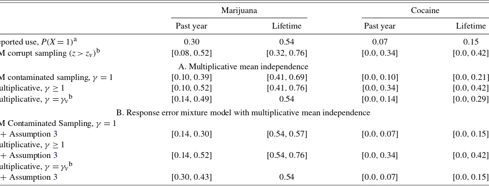
When the lower bound accurate reporting rate is coupled with the HM contamination assumption (Proposition1withγ=1), the bounds narrow considerably (Frame A). For lifetime mari-juana use, for example, the bounds narrow from[32%,76%]to [41%,69%], a 36% reduction in the width of the bounds. When we additionally impose the Assumption3response error mix-ture model (Frame B), the lifetime marijuana use rate is nearly point-identified, lying in the narrow range[54%,57%].
While powerful, the identifying assumption that drug use rates are identical among accurate and inaccurate reporters (γ =1) seems implausible. More realistically, the rate of il-licit drug use is higher among inaccurate reporters. Imposing the arguably innocuous assumption thatγ≥1, we can identify that the lifetime rate of marijuana use lies within[54%,76%], a 50% reduction in the range of uncertainty compared with the HM corrupt sampling bounds. For cocaine use, the restriction γ≥1 confers no identifying power compared with the corrupt sampling case.
Instead, one might assume that values ofγ found in Harri-son’s (1995) validation study of arrestees apply to the NHSDH sample. For cocaine consumption, imposing the valueγ=2.6 substantially reduces the range of uncertainty about its rate of use. The HM bounds only reveal that the rate of prior-year
co-caine consumption lies between 0% and 34%. Whenγ =2.6
under multiplicative mean independence Assumption2, the up-per bound falls to 14%, nearly a 60% reduction. This upup-per
Table 1. Bounds on the fractions of 18–24 year-olds using marijuana and cocaine
Marijuana Cocaine
Past year Lifetime Past year Lifetime
Reported use,P(X=1)a 0.30 0.54 0.07 0.15
HM corrupt sampling(z>zv)b [0.08,0.52] [0.32,0.76] [0.0,0.34] [0.0,0.42]
A. Multiplicative mean independence
HM contaminated sampling,γ=1 [0.10,0.39] [0.41,0.69] [0.0,0.10] [0.0,0.21] Multiplicative,γ≥1 [0.10,0.52] [0.41,0.76] [0.0,0.34] [0.0,0.42] Multiplicative,γ=γvb [0.14,0.49] 0.54 [0.0,0.14] [0.0,0.29]
B. Response error mixture model with multiplicative mean independence HM Contaminated Sampling,γ=1
+Assumption3 [0.14,0.30] [0.54,0.57] [0.0,0.07] [0.0,0.15] Multiplicative,γ≥1
+Assumption3 [0.14,0.52] [0.54,0.76] [0.0,0.34] [0.0,0.42] Multiplicative,γ=γvb
+Assumption3 [0.30,0.43] 0.54 [0.0,0.07] [0.0,0.15] aOffice of Applied Studies (2003).
bz
vandγvare the relevant values ofzandγfrom the validation studies discussed in the text.
A. Marijuana use, past year B. Marijuana use, lifetime
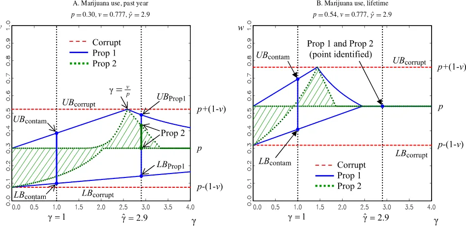
p=0.30,v=0.777,γˆ=2.9 p=0.54,v=0.777,γˆ=2.9
Figure 4. Bounds on marijuana use as a function ofγ.Note: These figures trace out sharp bounds on drug use prevalence rates as a function ofγ. The Proposition1bounds valuated atγ=1 are equivalent to Horowitz and Manski’s (1995) contaminated sampling bounds. The online version of this figure is in color.
bound falls further to 7%—nearly an 80% reduction—after ad-ditionally imposing the response error mixture model Assump-tion3. These results forγ=2.6 are very close to those under the untenable pure contamination assumption withγ=1. So, in this application, multiplicative mean independence has allowed us to substantially reduce uncertainty about the parameter with-out requiring an assumption that is nearly certain to be invalid.
A useful practical feature of Propositions 1 and 2 is that we can assess the sensitivity of the bounds to variation in
(γ ,zv). After all, Harrison’s estimates of misreporting may be
in error due to sampling variability and because her validation study might not accurately reflect misreporting rates in the gen-eral population. In sensitivity analysis, we considered how the Propositions1and2bounds vary withγ ∈ [0,4]over the four different outcome measures.
The results are traced out in Figure4for marijuana use (fig-ures for cocaine use available upon request). The most strik-ing results involve the bounds on incidence of lifetime mar-ijuana consumption. Under the response error Assumption3, we see from Figure 4B that if γ ≥1.85 the prevalence rate of lifetime use is identified to equal the self-reported rate of 0.54. Thus, ifγ=2.9, as revealed by Harrison, it follows that the prevalence rate among the general population is identified using data from the NHSDH. Moreover, this finding holds for allzv∈ [0.70,0.90]. Being able to point-identify lifetime mar-ijuana consumption follows from the Lemma1bounds, which reveal that for the range of parameters that apply in this setting (i.e.,z>0.5, γ ≥2, andp>0.5) everyone reports accurately. In fact, many researchers believe that measures of lifetime use are much less prone to reporting errors than shorter run mea-sures (e.g., Harrison1995). For cocaine use, the Proposition1 upper bound increases slightly with γ, whereas the Proposi-tion2bounds do not vary. Likewise, when assessing how the
bounds vary over zv∈ [0.70,0.90], we find that the Proposi-tion1upper bound on the probability of prior-year cocaine con-sumption falls from 15% to 9%, whereas the Proposition2 up-per bound does not vary.
5. CONCLUSION
In the contaminated sampling model studied by Horowitz and Manski (1995), the assumption that the outcome distribu-tion is independent of the mixing process has substantial identi-fying power. In many applications, however, this independence assumption is untenable. Yet when the independence assump-tion is discarded, the resulting bounds tend to be frustratingly wide. In this article, we introduce a general notion of a response error mixture model with multiplicative mean independence, with Propositions1and2characterizing the identifying power of these assumptions. Under these assumptions, we often find informative identification regions even when there is no prior information on the degree of accurate reporting. Moreover, we find that these assumptions can be easy to motivate and apply. Considering inference on the use of illicit drugs, our empirical illustration reveals that the multiplicative mean independence assumption can be credible and informative in environments where the pure contamination assumption is controversial.
Given the long-standing struggle to credibly address infer-ential problems that arise from response errors, we are hopeful that this nonparametric bounding framework can be usefully applied and extended. It is easy to think of variations on this theme that warrant study. For example, an interesting possibility might be to extend the idea of contaminated instruments used to evaluate treatment effects, as introduced by Hotz, Mullins, and Sanders (1997), to the case of multiplicative mean inde-pendence.
APPENDIX
Proof of Proposition1. If γ ≥1, both terms of the upper bound in Equation (6) monotonically decrease with the accu-rate reporting accu-rate,z. Thus, a closed form representation can be found by evaluating the mean outcome at the lowest pos-sible value of zsubject to the constraint implied by Assump-tion2that k0
there is no closed form bound that applies for all distributions (except when γ =1) because the two terms in Equation (6) move in opposite directions withz.
Analogously, ifγ ≤1 then both terms of the lower bound in Equation (6) increase withz. A closed form representation can be found by evaluating the mean outcome at the lowest possible value of the accurate reporting rate subject to the con-straint implied by Assumption2 that k0
γ ≤E(W|Z=1) ≤ per bound whenγ≤1, there is no closed form bound that ap-plies for all distributions (except whenγ=1) because the two terms in Equation (6) move in opposite directions withz.
Finally, if the conditions in Equation (7) are not satisfied,
z∈ [v,1)is not feasible. In that case,z=1 andE(W)=E(X).
Proof of Corollary 1. For binary outcomes, k0 =0 and k1=1. The HM bounds in Equation (3) becomep−minv{1−v,p}≤
v . The first γ-constraint inequality is always sat-isfied. When the second inequality is also satisfied, we have
P(W=1|Z=1)≤min{p−maxv{p−v,0},γ1}using the HM upper value, the upper bound isUB(v)(which does not exceed 1 since
p
we know that the upper bound equalsUB(v). In this case, when
γ≥1,UB(v)≤1≤p+γ (1−p). Second, consider the lower
bound whenγ >1. The functionLB(z)=p−minz{1−z,p}(1+ [1+ (γ−1)(1−z)])is concave inz∈ [0,1], and bounded between 0 whenz∈ [0,1−p]andpforz=1. Moreover,z∈ [γ (γ1−−1p),1) violate the restrictions in Equation (7); the HM lower bound p−min{1−z,p}
z exceeds
1
γ.Thus, the lower bound is attained by
settingz=vif the restriction in Equation (7) holds andz=1 otherwise.
Proof of Lemma1. The fraction of false positives is θ+=
P(X=1,Z=0)=(z(γ−+γp1)()z1−−γz), and the fraction of false
neg-Combining these results leads to the stated restrictions on allowed values ofz.
Lemma 2. (a) For p < γ1+1 and γ ≤ 1, w(z) is increas-ing within(−∞,γγ+1)and within(γγ+1,∞). Throughout, “in-creasing” means weakly increasing and “de“in-creasing” means weakly decreasing. Forp>γ1+1 andγ ≥1, w(z)is
it follows that: (f1) ∂∂wz|z=0 signs and imaginary otherwise. Using (f1) and (f2), we see that the slope ofw(z)has the same sign as 2(1−p)−γ atz=0 and
Lemma2(a) and (b),w(z)is monotonically increasing within (−∞,γγ+1)and within(γγ+1,∞)ifγ ≤1. Forγ >1,w(z)is
Lemma2(a) and (c), w(z)is monotonically decreasing within both(−∞,γγ w=patz=1. Lemma2establishes that any local extrema lie within[min{p,1−p},max{p,1−p}].
ACKNOWLEDGMENTS
The authors thank the valuable comments from an anony-mous referee, the editor, an associate editor, Phil Cross, Fran-cesca Molinari, Steve Stern, and seminar participants at George-town University, Iowa State University, and the University of Virginia. They also benefited from discussions at meetings of the Econometric Society and the Southern Economic Associa-tion. This research was supported in part by the Bankard Fund for Political Economy.
[Received September 2007. Revised May 2009.]
REFERENCES
Beresteanu, A., and Molinari, F. (2008), “Asymptotic Properties for a Class of Partially Identified Models,”Econometrica, 76, 763–814. [50]
Bollinger, C. (1996), “Bounding Mean Regressions When a Binary Variable Is Mismeasured,”Journal of Econometrics, 73, 387–399. [50]
Bound, J., Brown, C., and Mathiowetz, N. (2001), “Measurement Error in Sur-vey Data,” inHandbook of Econometrics, Vol. 5, eds. J. Heckman and E. Leamer, Amsterdam: Elsevier Science, Chapter 59, pp. 3705–3843. [49] Dominitz, J., and Sherman, R. (2004), “Sharp Bounds Under Contaminated or
Corrupted Sampling With Verification, With an Application to Environmen-tal Pollutant Data,”Journal of Agricultural, Biological, and Environmental Statistics, 9, 319–338. [49,50]
Frazis, H., and Loewenstein, M. (2003), “Estimating Linear Regressions With Mismeasured, Possibly Endogenous, Binary Explanatory Variables,” Jour-nal of Econometrics, 117, 151–178. [50]
Harrison, L. D. (1995), “The Validity of Self-Reported Data on Drug Use,”
Journal of Drug Issues, 25, 91–111. [56,57]
Hirsch, B. T., and Schumacher, E. J. (2004), “Match Bias in Wage Gap Esti-mates Due to Earnings Imputation,”Journal of Labor Economics, 22, 689– 722. [49]
Horowitz, J., and Manski, C. (1995), “Identification and Robustness With Con-taminated and Corrupted Data,”Econometrica, 63, 281–302. [49-52,57] Hotz, J., Mullin, C., and Sanders, S. (1997), “Bounding Causal Effects Using
Data From a Contaminated Natural Experiment: Analysing the Effects of Teenage Childbearing,”Review of Economic Studies, 64, 575–603. [57] Huber, P. (1981),Robust Statistics, New York: Wiley. [50]
Imbens, G., and Manski, C. (2004), “Confidence Intervals for Partially Identi-fied Parameters,”Econometrica, 72, 1845–1857. [50]
Kreider, B. (2007), “Partially Identifying the Prevalence of Health Insurance Given Contaminated Sampling Response Error,” working paper, Iowa State University. [55]
Kreider, B., and Pepper, J. (2007), “Disability and Employment: Reevaluating the Evidence in Light of Reporting Errors,”Journal of the American Statis-tical Association, 102, 432–441. [49,50]
(2008), “Inferring Disability Status From Corrupt Data,”Journal of Applied Econometrics, 23, 329–349. [49,50,55]
Lambert, D., and Tierney, L. (1997), “Nonparametric Maximum Likelihood Es-timation From Samples With Irrelevant Data and Verification Bias,”Journal of the American Statistical Association, 92, 937–944. [49,50]
Molinari, F. (2008), “Partial Identification of Probability Distributions With Misclassified Data,”Journal of Econometrics, 144, 81–117. [50,55] Mullin, C. H. (2005), “Identification and Estimation With Contaminated Data:
When Do Covariate Data Sharpen Inference?”Journal of Econometrics, 130, 253–272. [49]
Office of Applied Studies (2003), “Results From the 2002 National Survey on Drug Use and Health: National Findings,” NHSDA Series H-22, DHHS Publication SMA 03-3836, Substance Abuse and Mental Health Services Administration, Rockville, MD. [56]
Pepper, J. V. (2001), “How Do Response Problems Affect Survey Measurement of Trends in Drug Use?” inInforming America’s Policy on Illegal Drugs: What We Don’t Know Keeps Hurting Us, eds. C. F. Manski, J. V. Pepper, and C. Petrie, Washington, DC: National Academy Press, pp. 321–348. [56] Rosen, A. M. (2008), “Confidence Sets for Partially Identified Parameters That Satisfy a Finite Number of Moment Inequalities,”Journal of Econometrics, 146, 107–117. [50]
Stoye, J. (2009), “More on Confidence Intervals for Partially Identified Para-meters,”Econometrica, 77, 1299–1315. [50]