Full Terms & Conditions of access and use can be found at
http://www.tandfonline.com/action/journalInformation?journalCode=ubes20
Download by: [Universitas Maritim Raja Ali Haji] Date: 13 January 2016, At: 00:39
Journal of Business & Economic Statistics
ISSN: 0735-0015 (Print) 1537-2707 (Online) Journal homepage: http://www.tandfonline.com/loi/ubes20
Parameterized Expectations Algorithm and the
Moving Bounds
Lilia Maliar & Serguei Maliar
To cite this article: Lilia Maliar & Serguei Maliar (2003) Parameterized Expectations Algorithm and the Moving Bounds, Journal of Business & Economic Statistics, 21:1, 88-92, DOI:
10.1198/073500102288618793
To link to this article: http://dx.doi.org/10.1198/073500102288618793
View supplementary material
Published online: 01 Jan 2012.
Submit your article to this journal
Article views: 38
Parameterized Expectations Algorithm and
the Moving Bounds
Lilia M
aliar
and Serguei M
aliar
Departamento de Fundamentos del Análisis Económico, Universidad de Alicante, Campus San Vicente del Raspeig, Ap. Correos 99, 03080, Alicante, Spain
(maliarl@merlin.fae.ua.es and maliars@merlin.fae.ua.es)
The Parameterized Expectations Algorithm (PEA) is a powerful tool for solving nonlinear stochastic dynamic models. However, it has an important shortcoming: it is not a contraction mapping technique and thus does not guarantee a solution will be found. We suggest a simple modication that enhances the convergence property of the algorithm. The idea is to rule out the possibility of (ex)implosive behavior by articially restricting the simulated series within certain bounds. As the solution is rened along the iterations, the bounds are gradually removed. The modied PEA can systematically converge to the stationary solution starting from the nonstochastic steady state.
KEY WORDS: Nonlinear models; Numerical solutions methods; Optimal growth; Parameterized expectations algorithm.
1. INTRODUCTION
The Parameterized Expectations Algorithm (PEA) is a non-nite state space method for computing equilibria in nonlinear stochastic dynamic models (e.g., Wright and Williams 1982; Miranda and Helmberger 1988; Marcet 1988; den Haan and Marcet 1990; Christiano and Fisher 2000). The method is as follows: approximate the conditional expectation in Euler’s equation by a parametric function of state variables and nd the parameters, which minimize the distance between the expectation and the approximating function.
Several properties make the PEA an attractive tool for researchers in the area of economic dynamics. First, if a low-degree polynomial approximation delivers a sufciently accurate solution, the cost of the algorithm does not practi-cally depend on the dimensionality of the state space. Second, the PEA can be applied for analyzing not only the optimal economies but also the economies with externalities, distor-tions, liquidity constraints, and so on. Finally, the algorithm is fast and simple to program. For an extensive discussion of the method and its applications, see Marcet and Lorenzoni (1999) and Christiano and Fisher (2000).
The main drawback of the PEA is that it is not a contraction mapping technique and thus does not guarantee a solution will be found. In fact, if the assumed decision rule happens to be far from the true solution, the algorithm is likely to diverge. To achieve convergence, one has to wisely choose initial values for the parameters in the approximating function as well as a procedure for updating the parameters on each iteration.
To systematically nd a good initial point for iterations one can use homotopy: “[S]tart with a version of the model which is easy to solve, then modify these parameters slowly to go to the desired solution…. It is often possible to nd such ‘known’ solutions and to build a bridge that goes to the desired solution” (Marcet and Lorenzoni 1999, p. 156). One can also start from a solution that is previously computed by another numerical method, such as the log-linear approximation (see Christiano and Fisher 2000). It is evident, however, that the need to search for an initial point can seriously complicate implementing the PEA in practice.
This paper describes a simple modication that enhances the convergence property of the PEA. We consider the version of the algorithm developed by Marcet (1988) that evaluates the expectations by using Monte Carlo simulation. Our idea is to rule out the possibility of (ex)implosive behavior by articially restricting the simulated series within certain bounds. As the solution is rened along the iterations, the bounds are gradu-ally removed. We call this modication “moving bounds.”
Introducing the moving bounds resolves the problem of nding a good initial guess in the sense that the modied PEA is able to converge even if the initial guess is not very accu-rate. In our example, the modied PEA can systematically nd the stochastic solution starting from the nonstochastic steady state. It is also important to mention that the practical imple-mentation of the moving bounds is simple: one only has to automatically insert several lines in the original PEA code. In the remainder of the paper, we formally describe the modica-tion of the moving bounds and provide an illustrative example.
2. THE MOVING BOUNDS
We modify the PEA described in Marcet and Lorenzoni (1999) to include the moving bounds. Consider an economy, which is described by a vector ofnvariables,zt, and a vector
of s exogenously given shocks, ut. It is assumed that the
process8zt1 ut9is represented by a system
g4Et6”4ztC11 zt571 zt1 ztƒ11 ut5D01 for allt1 (1)
where g2 RmRnRnRs! Rq and ”2 R2n !Rm; the
vectorztincludes all endogenous and exogenous variables that
are inside the expectation, andut follows a rst-order Markov process. It is assumed thatzt is uniquely determined by (1) if the rest of the arguments is given.
©2003 American Statistical Association Journal of Business & Economic Statistics January 2003, Vol. 21, No. 1 DOI 10.1198/073500102288618793
88
Maliar and Maliar: Parameterized Expectations Algorithm 89
We consider only a recursive solution such that the condi-tional expectation can be represented by a time-invariant func-tionê4xt5DEt6”4ztC11 zt57, where xt is a nite-dimensional
subset of 4ztƒ11 ut5. If the function ê4¢5 cannot be derived analytically, we approximate ê4¢5 by a parametric function
–4‚1 x51 ‚2Rv. The objective will be to nd ‚ü such that
–4‚ü1 x5 is the best approximation to ê4x5 given the
func-tional form–4¢5,
‚üDarg min
‚2Rv
˜–4‚1 x5ƒê4x5˜0
This can be done by using the following iterative proce-dure.
¡ Step 1. Fix upper and lower bounds,zandzN, for the pro-cess8zt4‚51 ut9. For an initial iterationiD0, x ‚D‚4052
Rv. Fix initial conditionsu
0 and z0; draw and x a random series 8ut9TtD1 from a given distribution. Replace the condi-tional expectation in (1) with a function–4‚1 x5and compute the inverse of (1) with respect to the second argument to obtain
ztDh4–4‚1 xt4‚551 ztƒ11 ut50 (2)
¡ Step 2. For a given‚2Rv and given boundsz and zN,
recursively calculate8zt4‚51 ut9TtD1 according to
zt4‚5Dz if zt4‚5µz1
zt4‚5D Nz if zt4‚5¶z1N
zt4‚5Dh4–4‚1 xt4‚551 ztƒ11 ut5 if z < zt4‚5 <z0N
¡ Step 3. Find aG4‚5that satises
G4‚5Darg min
whereã4i5andSã4i5are the corresponding steps.
Iterate on Steps 2–5 until‚üDG4‚ü5andz < z
t4‚
ü5 <zN for
allt.
To perform Step 3, one can run a nonlinear least squares regression with the sample 8zt4‚51 ut9T
tD1, taking
”4ztC14‚51 zt4‚55as a dependent variable,–4¢5as an explana-tory function, and as a parameter vector to be estimated. We will not discuss the choice of the functional form for the approximation, the parameter number, the simulation length, and so on, as all of these are extensively analyzed in the pre-vious literature (e.g., Marcet and Lorenzoni 1999). Here, we focus only on the issue of convergence.
Thus, our modication is to articially restrict the simulated series, z < zt4‚ü5 <zN. If z and zN are set to ƒˆ and Cˆ,
respectively, the modied version is equivalent to the original one. The role of the bounds is discussed below.
Unlike the traditional value-iterative methods, the PEA does not have the property of global convergence. To be precise, if the approximation–4‚1 x5happens to be far from the true decision rule, ê4x5, then the simulated series 8zt4‚51 ut9TtD1 become highly nonstationary; as a result, the regression does not work appropriately and the algorithm diverges. Hence, one has to initially choose and subsequently update ‚ such that –4‚1 x5 remains sufciently close to the true decision rule, ê4x5. The need to fulll this requirement can compli-cate the use of the PEA in practice; for example, one has to search for an initial guess by using homotopy or the log-linear approximation.
We approach the problem from a different perspective. Specically, rather than trying to ensure that –4‚1 x5always remains close to ê4x5, we attempt to enhance the conver-gence property of the PEA and, consequently, to prevent the algorithm from failing if the approximation happens to be far from the true decision rule. The moving-bounds method exploits the fact that under the true decision rule, ê4x5, the process 8zt1 ut9TtD1 is stationary. The bounds articially induce the stationarity of possibly (ex)implosive simulated series8zt4‚51 ut9TtD1by not allowing such series to go beyond a xed range6z1z7N. This range is small, initially. However, it increases at each subsequent iteration. The bounds, therefore, play a stabilizing role at the beginning, when the approxima-tion–4‚1 x5is probably not accurate. As the PEA converges to the stationary solution, the bounds gradually lose their impor-tance and eventually become completely irrelevant.
In practice, there is no need to impose bounds on all of the simulated series. It is sufcient to restrict only the series for endogenous state variables, which are calculated by recursion and thus have a natural tendency to (ex)implode. In general, the remaining variables will be continuous functions of state variables and thus will be restricted automatically. Also, in some applications, there is no need to readjust (move) the bounds on each iteration. It is possible to x the bounds z
and zN at the beginning so that the algorithm will eventually converge.
We discuss a possible choice of the moving bounds param-eters in the next section. As an initial guess, we use the nonstochastic steady state. An advantage of this approach is that the initial point is computed in a simple and system-atic manner. The drawback is that the nonstochastic steady state solution can be far from the true stochastic solution, and, hence, the convergence can be slow. It is important to mention that using the steady state as an initial guess is not feasible within the original PEA framework.
3. AN EXAMPLE
To illustrate the application of the moving-bounds method, we consider the simplest one-sector stochastic growth model,
max
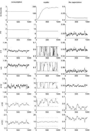
Figure 1. The Realization for Consumption, Capital, and the Expectation for a Single Stochastic Simulation (exploding capital, 1,000 periods).
where logˆtDlogˆtƒ1C…t with …t ¹N 401‘
25, the initial
condition4kƒ11 ˆ05 is given, and 240115. If the utility is logarithmic,ƒD1, and there is full depreciation of capital,
dD1, the model allows for an analytic solution: ct D41ƒ
„5ˆtk
tƒ1. In general, the closed-form solution to this model is not known.
The previous paper by den Haan and Marcet (1990) solves this model underƒD1 by using the PEA and the homotopy approach. They start from the solution to the model under
dD1 and change d from 1 to 0 in 10 steps; they calculate the solution for each step and employ it as the initial guess for the nextd.
We show how to solve the model by using the mod-ied version of the PEA. The program is written in
MATLAB and is available on both the ASA FTP data archive, ftp://www.amstat.org/, and the authors’ websites, http://merlin.fae.ua.es/maliarl and http://merlin.fae.ua.es/ marliars. Following den Haan and Marcet (1990), we approx-imate the conditional expectation by
Et6ctƒCƒ141ƒdCˆtC1k
ƒ1
t 57
ûexp4‚0C‚1logˆtC‚2logktƒ151 where ‚D4‚01 ‚11 ‚25is a vector of coefcients to be found. We can calibrate‚ as
‚0Dln
£ cƒƒ
ss 41ƒdCˆssk
ƒ1 ss 5
¤
1 ‚1D01 ‚2D00
Maliar and Maliar: Parameterized Expectations Algorithm 91
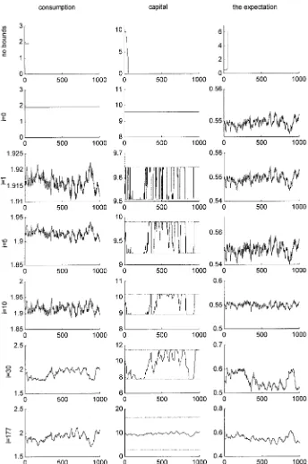
Figure 2. The Realization for Consumption, Capital, and the Expectation for a Single Stochastic Simulation (imploding capital, 1,000 periods).
However, to illustrate the convergence ability of the modied PEA, in the supplied MATLAB program, we draw‚1and‚2 from the normal distribution,N 40115. The algorithm has no difculty in converging starting from such a random initial condition.
The moving-bounds parameters are
k4i5Dkssexp4ƒai51 N
k4i5Dkss42ƒexp4ƒai551
where a >01 i is the number of iterations performed, and the variables with the subscript ss are the steady-state values.
Under this choice, on the rst iteration 4iD05, the simu-lated series coincide with the steady-state solution,kt4‚5Dkss, for all t. On the subsequent iterations, the lower and upper bounds gradually move, approaching 0 and 2kss, respectively. The parameteradetermines the pace at which the bounds are moved.
To simulate the model, we x the model’s parameters as follows:
„ ƒ d ‘ kƒ1 ˆ0
0.33 0.95 1 0.02 0.95 0.01 kss 1
We choose the updating PEA parameterŒD005. We set the moving-bounds parameter to aD00007, which corresponds approximately to having kD005zss and kN D105kss after 100 iterations. We x the length of simulation toT D11000 peri-ods. The convergence criterion used is that the L2 distance between vectors‚obtained in two subsequent iterations is less than 10ƒ5.
By construction, the moving-bounds modication may help the PEA to converge, although it may not affect the nal solution. Therefore, we will not provide any results regard-ing the properties of the solution; the discussion in den Haan and Marcet (1990, I994) applies to the modied PEA with-out changes. We shall just illustrate how the moving-bounds method works in practice.
Figures l and 2 show two examples of the stochastic simula-tions. The series plotted in each row are consumption, capital, and the value of the expression inside the conditional expec-tation, respectively. The rst row, “no bounds,” corresponds to the rst iteration of the original PEA, when no restrictions are imposed on the simulated series. The subsequent rows, “iD0,” “iD1,” and so on, are the simulated series obtained afteri iterations are performed. The last row shows the nal time series solution.
As we can see, when no restrictions are imposed, capital series become highly nonstationary. In the rst case (Fig. l), capital explodes quickly to almost 20 steady-state levels, whereas in the second case (Fig. 2), capital implodes to 0 in less than 100 periods. These graphs illustrate the problem of the initial point in the original PEA framework. To be spe-cic, our initial guess of the steady-state solution here proved to be inaccurate and led to nonstationary series that may not be used in the regression. It is not surprising, therefore, that the original PEA might have difculty in converging.
As follows from subsequent graphs, the poor initial guess does not create a problem for the modied PEA. Initially, at “iD0,” the bounds make the simulated series coincide with the steady state. On the next iteration, “iD1,” the possible range for capital increases; the capital series start uctuating and hitting the bounds. On subsequent iterations, the solu-tion renes and the range for capital continues to increase; the bounds are touched less and less frequently and, even-tually, are never in operation. At this point, the task of the moving bounds is completed, but the iterations continue until the required accuracy in the xed point is achieved.
One can easily check that our simple program is capa-ble of nding the solution under any meaningful values of
the model’s parameters. Furthermore, the property of conver-gence is not affected by a choice of the updating procedure; for example, one can assume full updating by settingŒD1. Finally, the algorithm has no difculty in converging when the simulation length increases to 10,000 or even to 100,000 periods.
4. CONCLUSION
This paper suggests a simple modication that enhances the convergence capability of the PEA. Specically, the mod-ied PEA does not suffer from the problem of the poor initial guess and can systematically converge starting from the non-stochastic steady-state solution. In the example considered, the property of convergence proved to be robust to all meaningful changes in both the model’s and the algorithm’s parameters. We discuss only one example; however, we nd the moving-bounds modication to be useful in several other applications.
ACKNOWLEDGMENTS
We thank Jeffrey Wooldridge, the associate editor, and an anonymous referee for valuable comments. We acknowledge the previous help of Albert Marcet in clarifying some issues related to the PEA. This research was partially supported by the Instituto Valenciano de Investigaciones Económicas and Ministerio de Ciencia y Technología, BEC 2001-0535. All errors are ours.
[Received March 2000. Revised May 2001.]
REFERENCES
Christiano, L., and Fisher, J. (2000), “Algorithms for Solving Dynamic Mod-els with Occasionally Binding Constraints,”Journal of Economic Dynam-ics and Control, 24, 1179–1232.
den Haan, W., and Marcet, A. (1990), “Solving the Stochastic Growth Model by Parameterizing Expectations,”Journal of Business and Economic Statis-tics, 8, 31–34.
den Haan, W., and Marcet, A. (1994), “Accuracy in Simulations,”Review of Economic Studies, 6, 3–17.
Marcet, A. (1988), “Solving Nonlinear Stochastic Models by Parameterizing Expectations,” unpublished manuscript, Carnegie Mellon University. Marcet, A., and Lorenzoni, G. (1999), “The Parameterized Expectation
Approach: Some Practical Issues,” inComputational Methods for Study of Dynamic Economies, eds. R. Marimon and A. Scott, New York: Oxford University Press, pp. 143–171.
Miranda, M., and Helmberger, P. (1988), “The Effect of Commodity Price Stabilization Programs,”American Economic Review, 78, 46–58. Wright, B., and Williams, J. (1982), “The Economic Role of Commodity
Storage,”Economic Journal, 92, 596–614.