Full Terms & Conditions of access and use can be found at
http://www.tandfonline.com/action/journalInformation?journalCode=ubes20
Download by: [Universitas Maritim Raja Ali Haji] Date: 11 January 2016, At: 23:07
Journal of Business & Economic Statistics
ISSN: 0735-0015 (Print) 1537-2707 (Online) Journal homepage: http://www.tandfonline.com/loi/ubes20
Tests for the Second Order Stochastic Dominance
Based on L-Statistics
José R. Berrendero & Javier Cárcamo
To cite this article: José R. Berrendero & Javier Cárcamo (2011) Tests for the Second Order
Stochastic Dominance Based on L-Statistics, Journal of Business & Economic Statistics, 29:2, 260-270, DOI: 10.1198/jbes.2010.07224
To link to this article: http://dx.doi.org/10.1198/jbes.2010.07224
Published online: 01 Jan 2012.
Submit your article to this journal
Article views: 110
View related articles
Tests for the Second Order Stochastic
Dominance Based on
L
-Statistics
José R. B
ERRENDEROand Javier C
ÁRCAMODepartamento de Matemáticas, Universidad Autónoma de Madrid, 28049 Madrid, Spain (joser.berrendero@uam.es;javier.carcamo@uam.es)
We use some characterizations of convex and concave-type orders to define discrepancy measures useful in two testing problems involving stochastic dominance assumptions. The results are connected with the mean value of the order statistics and have a clear economic interpretation in terms of the expected cumu-lative resources of the poorest (or richest) in random samples. Our approach mainly consists of comparing the estimated means in ordered samples of the involved populations. The test statistics we derive are func-tions ofL-statistics and are generated through estimators of the mean order statistics. We illustrate some properties of the procedures with simulation studies and an empirical example.
KEY WORDS: Convex order; Hypothesis testing; Lorenz order; Order statistics; Second order stochas-tic dominance.
1. INTRODUCTION
Stochastic orders were shown to be useful notions in several areas of economics, such as inequality analysis, risks analysis, or portfolio insurance. Since the beginning of the 1970’s, sto-chastic dominance rules have been an essential tool in the com-parison and analysis of poverty and income inequality. More recently, stochastic orders have also played an important role in the development of the theory of decision under risk and in actuarial sciences where they were used to compare and mea-sure different risks. Therefore, it is of major interest to acquire a deep understanding of the meaning and implications of the sto-chastic dominance assumptions. The construction of suitable empirical tools to make inferences about such assumptions is also clearly worthwhile.
The influential articles by Atkinson (1970) and Shorrocks (1983) are examples of theoretical works that provided a far-reaching insight into the importance of the stochastic domi-nance rules. In them, it was shown that the so called Lorenz dominancecan be interpreted in terms of social welfare for in-creasing concave, but otherwise arbitrary, income-utility func-tions. The book by Lambert (1993) also supplied a nice and general exposition on this subject and other topics related to the theory of income distributions. On the other hand, the books byGoovaerts, Kaas, and van Heerwaarden (1990),Kaas, van Heerwaarden, and Goovaerts(1994), and Denuit et al. (2005) provided different applications of stochastic orders to actuarial sciences and risk analysis.
From the empirical point of view, there are many articles in the econometric literature that propose different kinds of statis-tical tests for hypotheses involving different stochastic orders. In them, income distributions (or financial risks) are compared according to different criteria. For instance, Anderson (1996) used Pearson’s goodness-of-fit type tests whereas the approach in Barrett and Donald (2003) and inDenuit, Goderniaux, and Scaillet(2007) was inspired in the Kolmogorov–Smirnov sta-tistic. See alsoKaur, Prakasa Rao, and Singh(1994), McFad-den (1989), and Davidson and Duclos (2000) for other related procedures.
In this article we analyze convex and concave-type orderings between two integrable random variables X andY. We recall
thatXis said to beless or equal to Y in the convex orderand we writeX≤cxY, if E(f(X))≤E(f(Y)), for every convex func-tionf for which the previous expectations are well defined. The increasing convex order, to be denoted≤icx, is defined analo-gously, but imposing on the convex functions to be also nonde-creasing. By replacing “convex” by “concave” in the definitions above, we obtain theconcave order(≤cv) and the increasing concave order(≤icv).
The increasing convex and concave orders can be defined equivalently by
X≤icxY ⇐⇒
∞
t
Pr(X>u)du ≤
∞
t
Pr(Y>u)du, t∈R,
X≤icvY ⇐⇒
t
−∞
Pr(X≤u)du ≥
t
−∞
Pr(Y≤u)du, t∈R.
In this way, it is apparent that the increasing convex order com-pares the right tail of the distributions, while the increasing con-cave one focusses on the lowest part of the distributions. This difference leads to different uses of these two orders.
For instance, in actuarial sciences the risk associated to large-loss events is extremely important. Since convex functions take larger values when its argument is sufficiently large, ifX≤icxY holds, thenYis more likely to take “extreme values” thanX[see Corollary1(a) for the precise statement of this fact]. Therefore, the risk associated withX is preferable to the one withY. Ac-tually, the partial order relations≤icxand≤cx are extensively used in the theory of decision under risk, where they are called stop-loss orderandstop-loss order with equal means.
On the other hand, when comparing income distributions, it is sensible to analyze carefully the lowest part of the dis-tributions, that is, the stratus in the populations with less re-sources. This is the reason why the increasing concave order
© 2011American Statistical Association Journal of Business & Economic Statistics
April 2011, Vol. 29, No. 2 DOI:10.1198/jbes.2010.07224
260
is mainly considered in the literature of social inequality and welfare measurement under the name of thesecond order sto-chastic dominance. In this case, ifX≤icvY, the distribution of the wealth inY is considered to be more even than inX. If the populations to be compared have a different positive expecta-tion, it is very common to normalize them by dividing by their respective means and then check if they are comparable with respect to the concave order. This approach leads to theLorenz order, which is an essential tool in economics.
The convex and the concave orders are dual, and every prop-erty satisfied by one of them can be translated to the other one due to the relationships between the convex and the concave functions. Actually, it is easy to see thatX≤cxYif and only if Y≤cvX, andX≤icxYif and only if−Y≤icv−X.
In this work, we use some characterizations of the (increas-ing) convex and concave orders related to the mean order sta-tistics to define discrepancy measures useful in testing prob-lems involving stochastic dominance assumptions. The charac-terizations have a clear economic interpretation in terms of the expected cumulative resources of the poorest (or richest) in a randomly selected sample of individuals from the population. The considered discrepancy measures yield, in turn, a testing approach quite different from those quoted earlier. The estima-tors that appear are functions ofL-statistics and thus, in some situations, an asymptotic theory can be developed. However, in other cases, computational techniques such as bootstrap are also required.
The article is structured as follows: Section2includes some theoretical results linking the orderings with the mean order statistics. In Sections3and4we address two different testing problems: (a) testing whether two distributions are ordered with respect to the increasing convex or concave order versus the al-ternative that they are not, and (b) testing whether two distribu-tions are equal against the alternative that one strictly dominates the other. Sections5and6include various simulation studies. A real data example is considered in Section7. Section8 sum-marizes the main conclusions of the article. Finally, the proofs are collected in theAppendix.
2. CONVEX–TYPE ORDERS AND MEAN ORDER STATISTICS
Throughout the article,XandY are integrable random vari-ables with distribution functionsFandG, respectively, and we denote byF−1andG−1their quantile functions, i.e.,F−1(t):=
inf{x:F(x)≥t}, 0<t<1. For a real functionωon[0,1], we define
ω(X,Y):=
1 0
G−1(t)−F−1(t)ω(t)dt, (1) whenever the above integral exists. The following theorem shows that X ≤cxY is characterized by the fact that Equa-tion (1) is nonnegative for nondecreasing ω. Moreover, under a strict domination, ω(X,Y) is necessarily positive for
in-creasing weight functions. In the following, “=st” indicates the equality in distribution.
Theorem 1. Let I denote the class of nondecreasing real functions on[0,1]andI0the subset of functionsω∈Iwith the propertyω(0)≥0. Also,I∗stands for the subclass of strictly increasing functions ofIandI0∗:=I0∩I∗. We have:
(a) X≤cxY if and only ifω(X,Y)≥0, for allω∈I. The
equivalence remains true if “≤cx” and “I” are replaced by “≤icx” and “I0,” respectively.
(b) If X ≤cxY and ω(X,Y)=0 for some ω∈I∗, then
X=stY. The result still holds if “≤cx” and “I∗” are re-placed by “≤icx” and “I0∗,” respectively.
The distance in Equation (1) is closely related to the expected value of the order statistics. For k≥1, let (X1, . . . ,Xk) and
(Y1, . . . ,Yk)be random samples fromXandY, respectively.Xi:k
andYi:kdenote the associatedith order statistics,i=1, . . . ,k.
For k≥1 and 1 ≤m≤k, let us denote by Sm:k(X) [or sm:k(X)] the expectation of the sum of themgreatest (smallest)
order statistics, i.e.,
Sm:k(X):= k
i=k+1−m
EXi:k, sm:k(X):= m
i=1
EXi:k. (2)
If X measures the income level of the individuals in a popu-lation, the functionSm:k(X)[orsm:k(X)] is nothing, but the
ex-pected cumulative income of themrichest (poorest) individuals out of a random sample of sizekfrom the population. On the other hand, ifXis a risk,Sm:k(X)[orsm:k(X)] measures the
ex-pected loss of themlargest (lowest) loss events out ofkasX.
Corollary 1.
(a) WhenX≤icxY we have,Sm:k(X)≤Sm:k(Y), for allk≥
1 and 1≤m≤k. If additionallySm:k(X)=Sm:k(Y)for
somek≥2 and 1≤m<k, thenX=stY.
(b) WhenX≤icvY, we havesm:k(X)≤sm:k(Y), for allk≥
1 and 1≤m≤k. If additionally sm:k(X)=sm:k(Y)for
somek≥2 and 1≤m<k, thenX=stY.
The first statements in Corollary1(a) and (b) above are also consequences of corollary 2.1 in de la Cal and Cárcamo (2006). However, the second parts are new and required to derive the tests in Section4.
By using Theorem1 similar results can be obtained for the expected difference between the resources of the richest and the poorest. For instance,X≤icvY also implies that E(Yk:k− Y1:k)≤E(Xk:k−X1:k)for all k≥2. That is, the expected gap
between the resources of the richest and the poorest individ-ual (out ofk) is lower forY. Moreover, if this expected gap is equal for some k≥2, we necessarily haveX=stY. Some re-sults in the direction of Theorem1can also be found in Sordo and Ramos (2007).
3. TESTING STOCHASTIC DOMINANCE AGAINST NO DOMINANCE
When it is assumed that two populations are ordered, it is important to ensure that assumption is consistent with the data at hand. Accordingly, we consider the problem of testing the null hypothesisH0:X≤icxY against the alternativeH1:Xicx Y using two independent random samples X1, . . . ,Xn1 and
Y1, . . . ,Yn2 fromX andY, respectively. A test for the
second-order stochastic dominanceH0:X≤icvY versusH1:XicvY can be accomplished from the test considered in this section by just changing the sign of the data and exchanging the roles played byXandY. For relevant articles dealing with the same
testing problem we refer to Barrett and Donald (2003) and the references therein.
Our approach consists of comparing estimates of the mean order statistics of the two variables. Following the same lines as in the proof of lemma 4.4 in de la Cal and Cárcamo (2006), it is easy to give a characterization of the alternative hypothesis using the functionsSm:k(X)defined in Equation (2):
H1is true ⇐⇒ max
1≤m<k(Sm:k(X)−Sm:k(Y)) >0
for allk≥k0, (3) wherek0depends on the distribution of the variablesXandY.
As a consequence, a sensible procedure to solve the testing problem is to estimate the above quantity and rejectH0 when-ever the estimate is large enough. Suppose thatH1 holds and that the value of k is chosen so thatk→ ∞when n1,n2→ ∞. Due to Equation (3), we will eventually find a value of k for which there is at least a significant positive difference
Sm:k(X)−Sm:k(Y)(for somem), whereSm:k(X)andSm:k(Y)are
estimators of the quantities Sm:k(X)andSm:k(Y), respectively.
Hence, this procedure is expected to be asymptotically consis-tent. Indeed, the precise consistency result is established in the following.
We adopt a plug-in approach to estimateSm:k(X)andSm:k(Y)
and we replaceFandGwith the empirical distributionsFn1and
Gn2. That is,
In the end, our estimators areL-statistics since it can be readily shown that
Our proposal is to rejectH0when an appropriately normalized version ofˆk,n1,n2 is large enough, that is, we use the following is chosen so that the test has a preselected significance level,
α, in the limiting case under H0, i.e., in the case X =stY. The following result collects some properties of the test de-fined by the previous rejection region. The limits in the theo-rem are taken as n1 and n2 go to infinity in a way such that n1/(n1+n2)→λ∈(0,1). We note that the value ofk implic-itly depends onn1andn2since we have to estimate the expecta-tions of the order statistics EXi:kand EYi:kwith samples of sizes n1andn2, respectively. However, for the following asymptotic result it is only required that k→ ∞, without any additional restriction.
Theorem 2. Let X be a random variable such that
∞ earlier yields a consistent test under a condition only slightly stronger than the existence of the second moment. If one is only willing to assume E|X|γ <∞for some 1< γ <2, then the rate of convergence is slower and the consistency requires a slight modification to the test (see RemarkA.1in the Appen-dix). In such a case, the critical region in Equation (6) has to be The previous theorem does not require the variables to have finite support, neither does the continuity of the distrib-ution functions. However, it does not make any statement over the asymptotic size of the test, that is, it is not shown that lim supn1,n2→∞sup Pr(rejectH0)=α, where the supremum is
taken over allXandY under the null.
Theorem2assumes that we know the distribution of the test statistics whenX=stY so that we can determine the thresh-old valuecbeyond which we reject for each significance level
α. Unfortunately, it seems extremely difficult to derive such a distribution, which, in general, depends on the underlying un-known distribution of the data. To apply the test in practice we propose relying on a bootstrap approximation to simulate p -values, according to the following scheme:
1. Computeˆm,n1,n2 from the original samplesX1, . . . ,Xn1
2. Use these two parts to compute a bootstrap
version of the test statisticsˆ∗m,n
1,n2.
3. Repeat Step 2 a large numberBof times, yieldingB boot-strap test statisticsˆ∗m(,bn)1,n2,b=1, . . . ,B.
4. The p-value of the proposed test is given by p := Card{ ˆ∗m(,bn)1,n2 >ˆm,n1,n2}/B. We reject at a given level
αwheneverp< α.
The null hypothesis of the test is composite. By resampling from the pooled sample we approximate the distribution of our test statistics whenX=stY, which represents the least favor-able case forH0. If the probability of rejection in this case is approximatelyα, thenαis expected to be an upper bound for the probability of rejection under other less advantageous situa-tions. This idea is confirmed in the simulation study carried out in Section5. Similar bootstrap approximations were success-fully applied in a similar context in Abadie (2002) and Barrett and Donald (2003).
4. TESTING STOCHASTIC EQUALITY AGAINST STRICT DOMINANCE
In this section we want to test if two variables are equally distributed against the alternative that they are strictly ordered.
Hence, we provide a test for the null hypothesisH0:X=stY against the alternativeH1:X≤icxY andX=stY (or its dual, H1:X≤icvYandX=stY).
This kind of unidirectional test may appear naturally in eco-nomics where a certain change in the scenario, for example a change in tax policy or a technology shock, is expected to pro-duce a decrease or increase in the variability of the variables such as income or stock return, and therefore, is not unreason-able to assume that the distributions are ordered. The goal is to determine if they are different.
On other occasions we can apply a two-step procedure. First, we use the test described in Section3 to show that it is rea-sonable to assume that the variables are ordered and afterward apply this test. One possible solution to control the significance level of the final test is to use theBonferroni method. For exam-ple, to test the two hypotheses on the same data at 0.05 signif-icance level, instead of using ap-value threshold of 0.05, one would use 0.025.
It is important to remark that these tests use the additional information that the variables are ordered, and thus the cor-responding power is by far much higher than the power of the usual tests of equality of distribution, as the Kolmogorov– Smirnov test, for instance. Some illustrations regarding this question are included in Section6.3(see also Figure2).
Let us consider first the test for the increasing convex order. Theorem1and Corollary1provide a large number of potential discrepancy measures on which our test statistic can be based. Among them, we opted for a relatively simple one, namely, the difference between the expected value of the maximum ofk≥2 observations. By selectingm=1 in Corollary1(a), we obtain:
If X≤icxY, thenEXk:k≤EYk:k. Moreover, if additionally
EXk:k=EYk:kfor some k≥2, then X=stY.
Therefore, we consider the discrepancyk(X,Y):=EYk:k−
EXk:k,k≥2.k(X,Y)=0 underH0, whilek(X,Y) >0
un-derH1. A natural idea is to estimatek(X,Y)and reject H0 whenever the estimate is large enough. As before, to estimate
k(X,Y)we replaceFandGwith the empirical distributions, Fn1 andGn2. The resulting estimators are obtained by setting
j=kin Equation (4).
Theorem 3. Assume thatH0holds and that the common dis-tributionFsatisfies
∞
−∞
F(x)2k−2x2dF(x) <∞. (10)
Assume also thatn1/n tends to λ∈(0,1), as n→ ∞, where n:=n1+n2. LetUbe a random variable uniformly distributed on(0,1). Define the random variable
where the symbol−→dstands for the convergence in
distribu-tion and N(0, σW2)is a normal random variable with mean 0 and varianceσW2.
Hence, to testH0againstH1we can use the simple critical region
of the standard normal distribution that depends on a suitable significance level.
To estimateσWwe proceed as follows: givenUwith uniform
distribution on(0,1), we obtain a pseudo-value ofW,Wˆ, by re-placing in Equation (11) the unknown true distributionFby the pooled empirical distributionFn,n=n1+n2, computed from the observations of the two samples (since underH0both sam-ples come from the same distribution). LetZ1:n≤ · · · ≤Zn:nbe
the order statistics of the pooled sample. After some computa-tions,Wˆ can be expressed as
ˆ
Equation (9). Finally, we generate a large number of pseudo-values and compute its standard deviation. According to our computations, 5000 pseudo-values are enough to obtain a pre-cise estimateσˆW. The consistency of this estimator is analyzed
in PropositionA.1of theAppendix.
If we are interested in the alternative hypothesisH1:X≤icvY and X=stY, some modifications of the procedure described earlier are needed. In this case, the appropriate discrepancy measures areŴk:=EY1:k−EX1:k,k≥2. This quantity can be
where now the weights are given by
γi,k,n:=
Comparing Equation (9) with Equation (14) we see that when we are interested in the second-order dominance we use anL -statistic that places more weight on the lowest order -statistics, whereas for the increasing convex order the highest order sta-tistics receive more weight.
The proof of the following theorem is analogous to that of Theorem3so that it is omitted.
Theorem 4. Assume thatH0holds and that the common dis-tributionFsatisfies
∞
−∞
(1−F(x))2k−2x2dF(x) <∞. (15)
Assume also that n1/n tends toλ∈(0,1), as n→ ∞, where n:=n1+n2. LetUbe a random variable uniformly distributed on(0,1). Define
V:= −k(1−U)k−1F−1(U)+k(k−1)
1
U
(1−t)k−2F−1(t)dt,
and letσV2be the variance ofV. Then, asn1→ ∞,
(1/n1+1/n2)−1/2Ŵˆk,n1,n2−→dN(0, σ
2
V).
The procedure to estimate the asymptotic standard deviation
σV is also analogous to that proposed forσW. In this case the
pseudo-values are
ˆ V= −k
1−⌈nU⌉ n
k−1
Z⌈nU⌉:n+k n
⌈nU⌉+1
γi,k−1,nZi:n,
whereγi,k−1,nis defined in Equation (14). For an appropriate
normal quantilez,H0is rejected in the critical region{(1/n1+ 1/n2)−1/2Ŵˆk,n1,n2/σˆV>z}.
An appealing aspect of Theorem4is that it guarantees the as-ymptotic normality of the test statistic under remarkably mild conditions. For instance, when the variables are nonnegative (which is the case of most interesting economic variables) the condition EX<∞impliesx[1−F(x)] →0 asx→ ∞, which in turn implies Equation (15) fork≥2. Therefore, in this impor-tant case, the finiteness of the expectation is all that is needed to ensure the asymptotic normality, whereas the asymptotic be-havior of most related test statistics in the literature involves the existence of the second moment. See for instance, Aly (1990, theorem 2.1), Marzec and Marzec (1991, theorem 2.1), and Belzunce, Pinar, and Ruiz (2005, theorem 2.1).
5. MONTE CARLO RESULTS: STOCHASTIC DOMINANCE AGAINST NO DOMINANCE
To investigate the properties of the test of Section 3 for small samples, we carried out a simulation study inspired by that of Barrett and Donald (2003). We consider the test for the second-order stochastic dominance H0:X ≤icv Y versus H1:XicvY across five different models (M1–M5). The mod-els are related to lognormal distributions, which are frequently found in welfare analysis. We consider three mutually inde-pendent standard normal variablesZ,Z′, andZ′′. In all mod-els X=exp(0.85+0.6Z) is fixed. In the first three models, Y =exp(μ+σZ′)is also lognormal. The models only differ in the values of the parametersμandσ:
• M1:μ=0.85 andσ=0.6. Hence,H0is true andX=stY. • M2:μ=0.6 andσ=0.8. In this case,H0is false. • M3: μ=1.2 andσ =0.2. In this model,H0 is true but
X=stY.
In the last two models,Yis a mixture of two lognormal dis-tributions:
Y=1{U≥0.1}exp(μ1+σ1Z′)+1{U<0.1}exp(μ2+σ2Z′′), where 1Astands for the indicator function of the setA,U is a
uniform[0,1]random variable also independent of the normal variablesZ,Z′, andZ′′.
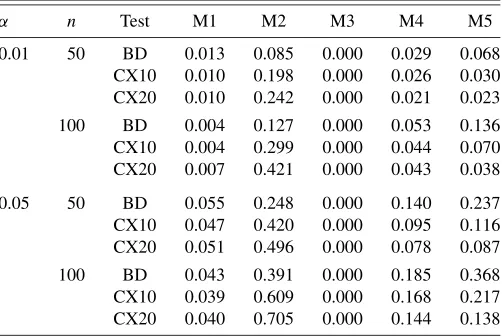
Table 1. Rejection rates for BD, CX10, and CX20 tests with bootstrapp-value under models M1–M5
α n Test M1 M2 M3 M4 M5
0.01 50 BD 0.013 0.085 0.000 0.029 0.068 CX10 0.010 0.198 0.000 0.026 0.030 CX20 0.010 0.242 0.000 0.021 0.023
100 BD 0.004 0.127 0.000 0.053 0.136 CX10 0.004 0.299 0.000 0.044 0.070 CX20 0.007 0.421 0.000 0.043 0.038
0.05 50 BD 0.055 0.248 0.000 0.140 0.237 CX10 0.047 0.420 0.000 0.095 0.116 CX20 0.051 0.496 0.000 0.078 0.087
100 BD 0.043 0.391 0.000 0.185 0.368 CX10 0.039 0.609 0.000 0.168 0.217 CX20 0.040 0.705 0.000 0.144 0.138
• M4:μ1=0.8, σ1=0.5,μ2=0.9, andσ2=0.9. In this case,H0is false.
• M5:μ1=0.85,σ1=0.4, μ2=0.4, andσ2=0.9. Here H0is again false.
We simulated samples with sizes n1=n2=50 and n1= n2=100, and then we applied the test based on Equation (6) withk= ⌈n1/10⌉(denoted by CX10), withk= ⌈n1/20⌉ (de-noted by CX20), and a test proposed by Barrett and Donald (2003) for the same testing problem (denoted by BD). We used the bootstrap scheme described in Section 3 with B=1000 to approximate thep-value. Accordingly, we have selected the Barrett–Donald test using the same bootstrap scheme, namely, the one called KSB2 in that article.
For each model, we performed 1000 Monte Carlo replica-tions of the experiment and recorded the rejection rates at the significance levelsα=0.01 andα=0.05 for both tests. The results can be found in Table1.
Both tests behave similarly underH0: under M1 we obtain rejection rates not far from the nominal significance levels. This suggests that the bootstrap approximation works well for the three tests. Under M3,H0is true butX=stY so that we expect a rejection rate below the nominal significance level. Observe that the tests never rejectH0in this case. Regarding models for whichH1 is true, neither of the tests is uniformly better than the others: CX10 and CX20 are more powerful than BD under M2, but BD is more powerful than CX10 and CX20 under the mixtured models M4 and M5.
6. MONTE CARLO RESULTS: STOCHASTIC EQUALITY AGAINST STRICT DOMINANCE We carried out a simulation study to assess the performance of the tests proposed in Section4for finite sample sizes. Also, we want to illustrate some ideas about the choice of the para-meterk.
6.1 General Description and Results for Fixedk
We considered a situation in whichX has a Weibull distri-bution with shape parameter 10 and scale parameter 1/ Ŵ(1+ 1/10). On the other hand, Y has a Weibull distribution with shape parameter θ and scale parameter 1/ Ŵ(1 +1/θ ), for
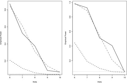
Figure 1. Empirical power curves for the test in Equation (13) under different Weibull alternatives, sample sizes 50 and 100, and several values ofk.
θ=6,8,10. The scale parameters were chosen so that EX= EY=1, which is the most unfavorable situation to detect de-viations fromH0. The null hypothesis corresponds toθ=10. All the considered pairs of variables are ordered since they have the same mean and the difference between their density func-tions has two crossing points (see Shaked and Shanthikumar 2006, theorem 3.A.44, p. 133). For all the described combina-tions, we simulate couples of independent samples with sizes n1=n2=50,100 and apply the test based on the critical re-gion in Equation (13) fork=2,4,6,10 at the significance level
α=0.05. After replicating this experiment 1000 times, we reg-istered the proportion of times for whichH0was rejected, that is, the empirical power of the tests.
In Figure1the resulting empirical power curves (n1=n2= 50 andn1=n2=100) are represented. The horizontal dotted line corresponds to the nominal significance level of the test. From the results of the experiment it is apparent that the largest values ofkperform clearly better than the smallest ones. How-ever, askincreases the improvement seems to be less signif-icant. These results point out that the power of the test may strongly depend on the value ofk. In the following section we address the problem of choosing an appropriate value of this parameter.
We also performed similar simulation studies with both gamma and Student’strandom variables. The results were re-markably similar and are omitted for the sake of brevity.
6.2 Data-Driven Selection ofk
There are two factors that should be taken into account in the selection ofk. The first one is the ability of the discrepancy
measurek(X,Y)to detect deviations from the null hypothesis.
From this point of view we should choose the valuekthat max-imizesk(X,Y). In some important situations it can be shown
thatk(X,Y)increases withkand then we should choosekas
large as possible in these cases. However, since X andY are unknown, in practice, we use the estimateˆk,n1,n2 instead of
k(X,Y). Therefore, another important factor to be considered
is the variability ofˆk,n1,n2. It is intuitively clear that ask
in-creases (for fixed n1 and n2), it is more difficult to estimate
k(X,Y)so that an increase in the variance ofˆk,n1,n2 should
be expected. As a consequence, a large value ofkmight not be a good choice regarding this second aspect. The results displayed in Figure1collect the overall effect of the two factors under the Weibull model.
A simple measure to quantify which of the two factors is more influential is the inverse of the coefficient of variation. IfXis a random variable with finite second moment, we denote by CV−1:=EX/σX the inverse of the coefficient of variation
(σX being the standard deviation ofX). Let us denote by CV−k1
the inverse of the coefficient of variation of the test statistics ˆ
k,n1,n2 given in Equation (8). Overall, a high value of CV−
1
k
can generate a test with a good power. A reasonable data-driven choice ofkwill then be the value ofkthat provides the high-est high-estimated value of CV−k1. In practice, a standard bootstrap procedure can be used to estimate CV−k1.
A hindrance of this approach is that the asymptotic result for fixedkderived in Section4is no longer applicable. The proce-dure described above automatically selects a value ofk“against the null” so that the critical value prescribed by Equation (13)
Table 2. Rejection rates for the test of equality against strict dominance whenkis automatically selected
Weibull θ=6 θ=8 θ=10
n1=n2=50 0.845 0.309 0.067
n1=n2=100 0.988 0.542 0.052
NOTE: The nominal significance level isα=0.05. The last column corresponds to the null hypothesis.
is too liberal. Again, bootstrap techniques may help to approxi-mate the appropriate critical value for a given significance level. The method is fairly similar to the one described in Section3 and the details are omitted.
Since we use bootstrap both for estimating the coefficient of variation and for approximating the critical level, our procedure is computationally expensive. Fortunately, using a small num-ber of bootstrap samples yields acceptable results. In Table2, we report the empirical significance level and power of the test, withkautomatically selected as described above using only 10 bootstrap samples to estimate the coefficient of variation and 200 bootstrap samples to approximate the critical value. The experiment was replicated 1000 times andα=0.05 is the nom-inal significance level. We see that the data-driven selection of kyields good power and at the same time allows us to control the significance level.
6.3 Comparison With the Kolmogorov–Smirnov Test As it was mentioned at the beginning of Section4, the tests generated by this approach take into account the important in-formation of the ordering between the two variables. Therefore,
the power of these tests is expected to be higher than the power of the usual omnibus tests for equality of the distributions in the literature (which work against all and not just ordered al-ternatives). To illustrate this point, we compared the empiri-cal power of our test (both with fixedk=10 and data-driven selected k) with that of the Kolmogorov–Smirnov test under the Weibull model described in Section6.1with sample sizes n1=n2=50,100. The results are summarized in Figure2. We see that the tests proposed in this section have (uniformly) by far a much higher power than the Kolmogorov–Smirnov test. Note also that the automatic procedure to selectkyields similar results to the casek=10 (which is the best one across all the considered values, see Figure1).
7. AN EMPIRICAL EXAMPLE
To illustrate the tests of Sections 3 and 4, we discuss a dataset previously considered in Barrett and Donald (2003). The dataset is drawn from theCanadian Family Expenditure Surveyfrom the years 1978 and 1986. We are interested in the comparison of the income distributions in these years.
We normalize incomes by dividing the data in each sample by its average and analyze whether the resulting distributions are ordered with respect to the concave order. This is equivalent to comparing the distributions according to the Lorenz order.
Some descriptive graphics of the normalized incomes can be found in Figure3. In the panels on the left we plotted the em-pirical distribution functions for the pre-tax and post-tax nor-malized income data. The corresponding kernel density esti-mates are plotted in the right panels. Notice that the empiri-cal distribution functions for 1978 and 1986 are rather similar.
Figure 2. Empirical power curves for the test in Equation (13) with fixedk=10 (solid line), automatic selection ofk(dotted–dashed line), and the Kolmogorov–Smirnov test (dashed line) under the Weibull model. The sample sizes aren1=n2=50 (left) and 100 (right). The horizontal dotted line corresponds to significance levelα=0.05.
Figure 3. Empirical distribution functions and kernel density estimates for pre-tax and post-tax income data in 1978 and 1986.
From the estimated densities we notice that qualitative aspects of both distributions (positive skewness, slight bimodality) are also comparable.
Figure4displays the difference between the integrated em-pirical quantile functions of the normalized samples. This dif-ference is exactly the empirical counterpart of the function given in Lemma A.1 in the Appendix. This function is, for
the most part, positive and this fact suggests that both distrib-utions can be ordered according to the Lorenz order. A more formal evaluation of this ordering property can be achieved by applying the test developed in Section3. The null hypoth-esis is that the income distribution of 1978 dominates in the Lorenz order that of 1986. To be more precise, if X1978 and X1986 denote the variables in the years 1978 and 1986, we
Figure 4. Difference between the integrated quantile functions (1986 minus 1978).
Table 3. p-values for testing the null hypothesis that the income distribution of 1978 dominates in the Lorenz order that of 1986
versus the alternative that both distributions are not ordered
k ⌈min{n1,n2}/100⌉ ⌈min{n1,n2}/500⌉ ⌈min{n1,n2}/1000⌉
Before tax 0.666 0.628 0.636 After tax 0.590 0.592 0.598
testH0:X1986/EX1986≤cvX1978/EX1978againstH1: notH0(or equivalently, H0:X1978/EX1978≤cxX1986/EX1986 against the same alternative). Therefore, we applied the test based on the critical region in Equation (6), where the critical valuecwas approximated usingB=500 bootstrap samples. Also, several values of kwere considered. The corresponding p-values are displayed in Table3.
Since thep-values are quite large, the conclusion is that the null hypothesis cannot be rejected. This also means that the neg-ative parts of the functions depicted in Figure4are not signifi-cant. Thep-values are almost the same for the considered values ofk. Moreover,p-values are also similar when considering the after tax or before tax incomes.
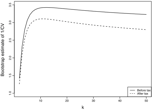
Since the assumption that both distributions are ordered is acceptable, a natural question is if the distributions are equal (according to this order), or if onestrictlydominates the other. We note that the equality for the Lorenz order is the equality in distribution up to dilations of the variables. To answer this question we use the test introduced in Section4. We used boot-strap estimates (based onB=500 resamples) of the inverse of the coefficient of variation of the discrepancies, as described in Section6.2, to explore which values ofkare more suitable. A graphical representation of these estimates can be found in Figure5. It turns out that the maximum is attained atkˆ=14 (be-fore tax) andˆk=11 (after tax). Accordingly, we carry out the tests corresponding to these values where thep-values are ap-proximated using, again, bootstrap. The resultingp-values are 0.006 (before tax) and 0.002 (after tax). Therefore, our conclu-sion is that the income distribution in 1978 strictly dominates that of 1986, according to Lorenz order. In this sense, we con-clude that the income distribution in 1978 was more even than in 1986. The conclusion does not depend upon the mean in-come level since we used normalized inin-comes and neither upon
Figure 5. Bootstrap estimates of the inverse of the coefficient of variation ofˆk,n1,n2as a function ofk.
the consideration of incomes before tax nor after tax. Moreover, we can assert thatX1986=staX1978, for alla>0, that is, the sit-uation in 1986 was not a dilation of that in 1978.
8. CONCLUSION
We propose a new approach to solve two different testing problems related to the second-order stochastic dominance. First, we discuss a test for stochastic dominance versus no dominance. The technique consists of comparing the estimated expected cumulative resources of them-poorest in random sam-ples of sizekof the populations. We derive the asymptotic con-sistency of the method and approximate thep-values via boot-strap. The simulation studies show that the methodology works well. However, in this work the asymptotic consistency of the considered bootstrap scheme is not proved. The selection of the tuning parameterkaffects the power of the resulting test and further research will be needed to understand better the influ-ence of this parameter. Also, we consider a test of stochastic equality against strict domination. In this case, we compare the estimated expected maxima or minima of random samples of sizekof the populations. The estimators of the discrepancies areL-statistics and we show that their distributions are asymp-totically normal (for allk). Again, the choice ofkhas an impact on the power of the tests. For this reason, we derive a data-driven selection ofkto obtain a value of this parameter gener-ating a powerful test. One important advantage of this last test is that it is much more powerful than the usual tests of equality in distribution since we include the additional information that the variables are stochastically ordered.
APPENDIX: PROOFS
Without loss of generality we assume the functionsω∈I are right continuous. Forω∈I,μω is the Lebesgue–Stieltjes
measure defined byμω((a,b])=ω(b)−ω(a),(a,b] ⊂ [0,1].
The following lemma is a consequence of the results in Rüschendorf (1981), where 1Astands for the indicator function
of the setA.
Lemma A.1. X≤cxYif and only if1(t,1](X,Y)≥0, for 0≤
t<1, with equality for t=0. The equivalence remains true if “≤cx” is replaced by “≤icx” and the restriction for t=0 is dropped.
Lemma A.2. Letf be a continuous and nonnegative function on[0,1]. If[0,1]fdμω=0,for some ω∈I∗, thenf ≡0 on
[0,1].
Proof. If for somet0∈ [0,1],f(t0) >0, by the continuity of f there exists a nonempty interval(a,b] ⊂ [0,1]such thatf>0 on (a,b]. Since ω∈I∗, we have μω((a,b]) >0. Therefore,
f >0 on an interval with positive measure, which contradicts the assumption on the value of the integral.
Proof of Theorem1
We restrict to the case X≤icxY. The proof for the convex order is analogous taking into accountX≤cxY if and only if X≤icxY and EX=EY. From LemmaA.1,ω(X,Y)≥0 for
allω∈I0impliesX≤icxY. For the reverse implication, let us
this completes the proof of Corollary1(a).
To show Corollary 1(b), let us assume that X≤icx Y and there exists a function ω∈I0∗ such that ω(X,Y)=0. By
Equation (A.1), we have [0,1]1(s,1](X,Y)dμω(s)=0. By
LemmaA.1, the function1(·,1](X,Y)is nonnegative on[0,1]
and it is trivially continuous. We apply Lemma A.2 to con-clude1(·,1](X,Y)≡0 on[0,1]. This impliesF− Cal and Cárcamo (2006, lemma 4.3), we obtain
Sm:k(Y)−Sm:k(X)=ω(X,Y)
withω(t)=kPr(βk−m:k−1≤t), (A.2) whereβk−m:k−1 (m<k) is a Beta(k−m,m) random variable andβ0,k−1is degenerate at 0. This implies thatω∈I0and for k≥2 and 1≤m<k, ω∈I0∗. Hence, Corollary1(a) follows from Theorem1. Corollary1(b) is analogous.
Proof of Theorem2
We only give a proof for Theorem2(a) since Theorem2(b) is analogous. Given a random sampleX1, . . . ,Xn1(orY1, . . . ,Yn1)
empirical distribution and quantile functions of the sample. By Equations (A.2) and (1), for allmandk, we obtain orem 2.1(b) in delBarrio, Giné, and Matrán (1999) ensured
that fori=1,2 the sequences{√ni
∞
−∞|F(t)−Fni(t)|dt}ni≥1 are bounded in probability. This directly implies that{(1/n1+ 1/n2)−1/2| ˆk,n1,n2|}n1,n2≥1 is bounded in probability. Hence
the valuecthat appears in Equation (6) is bounded.
On the other hand, ifH1is true, a similar argument as in the proof of lemma 4.4 in de la Cal and Cárcamo (2006) shows that there exist anǫ0>0 and a positive integerk0such that for all k≥k0
1
k1max≤m<k{Sm:k(X)−Sm:k(Y)}> ǫ0. (A.4)
A similar reasoning as in Equation (A.3), the integrability ofX and Glivenko–Cantelli yield
Forn1andn2large enough, Equation (A.5) ensures that for all mandk
region is determined by a bounded quantityc, we conclude that Theorem2(a) holds and the proof is complete.
Remark A.1. Under the condition E|X|γ <∞for some 1< γ <2 instead of0∞√Pr(|X|>x)dx<∞, the same proof, but using theorem 2.2 in delBarrio, Giné, and Matrán(1999) yields the consistency of the test given by the critical region in Equa-tion (7).
Proof of Theorem3
First, we shall show that the L-statistic n1
i=1ωi,k,n1Xi:n1,
Next, we apply Li, Rao, and Tomkins(2001, theorem 2.1)
withW defined in Equation (11). For the last equality, take into account that and the second term is not random. The condition in Equation (10) is needed to ensure that conditions (i)–(iii) inLi, Rao, and Tomkins(2001, theorem 2.1) hold. By the asymptotic equiva-lence established earlier and the assumptionn1/n→λwe also have
Following the same lines, we can also show
√
Finally, since both samples are independent, we deduce √
nˆk,n1,n2 −→dN
0, σW2/[λ(1−λ)], n→ ∞,
which in turn implies Equation (12).
The next proposition shows the consistency of the estimators of the asymptotic standard deviationsσW andσV described in
Section4. Although we ask for a finite second moment we be-lieve the conditions in Equations (10) and (15) are enough.
Proposition A.1. If the variableXhas finite second moment, the estimatorsσˆW andσˆV described in Section4are consistent. Proof. We only give a proof for σˆW since the one for σˆV
is analogous. If EX2<∞, it is easy to check that EW2<∞, whereW is defined in Equation (11). Therefore, recalling that
ˆ
Wis the empirical counterpart ofW, we only need to show that E(Wˆ −W)2→0, as the sample sizen→ ∞. Some computa-tions show
E(Wˆ −W)2≤k2F−n1−F−122+k2(k2−1)F−n1−F−11, whereF−n1is the empirical quantile function and · 1, · 2 stand for theL1andL2norms, respectively. The existence of the second moment ofX guarantees that F−n1−F−12,F−n1− F−11→0, asn→ ∞and the proof is complete.
ACKNOWLEDGMENTS
The authors thank the referees and the associated editor of the journal for their valuable comments and suggestions, which have led to an improved version of the article. Furthermore, they pointed out to us the importance of the testing problem discussed in Section3.
This research was supported by the Spanish MEC grants MTM2007-66632 and MTM2008-06281-C02-02 and Comu-nidad de Madrid grant S-0505/ESP/0158.
[Received September 2007. Revised September 2009.]
REFERENCES
Abadie, A. (2002), “Bootstrap Tests for Distributional Treatment Effects in In-strumental Variable Models,”Journal of the American Statistical Associa-tion, 97, 284–292. [262]
Aly, E.-E. A. A. (1990), “A Simple Test for Dispersive Ordering,”Statistics & Probability Letters, 9, 323–325. [264]
Anderson, G. (1996), “Nonparametric Tests of Stochastic Dominance in In-come Distributions,”Econometrica, 64, 1183–1193. [260]
Atkinson, A. B. (1970), “On the Measurement of Inequality,”Journal of Eco-nomic Theory, 2, 244–263. [260]
Barrett, G. F., and Donald, S. G. (2003), “Consistent Tests for Stochastic Dom-inance,”Econometrica, 71, 71–104. [260,262,264,266]
Belzunce, F., Pinar, J. F., and Ruiz, J. M. (2005), “On Testing the Dilation Order and HNBUE Alternatives,”Annals of the Institute of Statistical Mathemat-ics, 57, 803–815. [264]
Davidson, R., and Duclos, J. Y. (2000), “Statistical Inference for Stochastic Dominance and for the Measurement of Poverty and Inequality,” Econo-metrica, 68, 1435–1464. [260]
de la Cal, J., and Cárcamo, J. (2006), “Stochastic Orders and Majorization of Mean Order Statistics,”Journal of Applied Probability, 43, 704–712. [261, 262,269]
del Barrio, E., Giné, E., and Matrán, C. (1999), “Central Limit Theorems for the Wassertein Distance Between the Empirical and the True Distribution,”
The Annals of Probability, 27, 1009–1071. [269]
Denuit, M., Dhaene, J., Goovaerts, M., and Kass, R. (2005),Actuarial Theory for Dependent Risks, New York: Wiley. [260]
Denuit, M., Goderniaux, A. C., and Scaillet, O. (2007), “A Kolmogorov– Smirnov-Type Test for Shortfall Dominance Against Parametric Alterna-tives,”Technometrics, 49, 88–99. [260]
Goovaerts, M. J., Kaas, R., and van Heerwaarden, A. E. (1990),Effective Actu-arial Methods, Amsterdam: North-Holland. [260]
Kaas, R., van Heerwaarden, A. E., and Goovaerts, M. J. (1994),Ordering of Actuarial Risks. Cairo Education Series, Amsterdam: University of Ams-terdam. [260]
Kaur, A., Prakasa Rao, B. L. S., and Singh, H. (1994), “Testing for Second-Order Stochastic Dominance of Two Distributions,”Econometric Theory, 10, 849–866. [260]
Lambert, P. J. (1993),The Distribution and Redistribution of Income, a Math-ematical Analysis (2nd ed.), Manchester: Manchester University Press. [260]
Li, D., Rao, M. B., and Tomkins, R. J. (2001), “The Law of the Iterated Loga-rithm and Central Limit Theorem forL-Statistics,”Journal of Multivariate Analysis, 78, 191–217. [270]
Marzec, L., and Marzec, P. (1991), “On Testing Equality in Dispersion of Two Probability Distributions,”Biometrika, 78, 923–925. [264]
McFadden, D. (1989), “Testing for Stochastic Dominance,” inStudies in the Economics of Uncertainty: In Honor of Josef Hadar, eds. T. B. Fomby and T. K. Seo, New York–Berlin–London–Tokyo: Springer. [260]
Rüschendorf, L. (1981), “Ordering of Distributions and Rearrangement of Functions,”The Annals of Probability, 9, 276–283. [268]
Shaked, M., and Shanthikumar, J. G. (2006),Stochastic Orders. Springer Series in Statistics, New York: Springer. [265]
Shorrocks, A. F. (1983), “Ranking Income Distributions,”Economica, 50, 3– 17. [260]
Sordo, M. A., and Ramos, H. M. (2007), “Characterization of Stochastic Orders byL-Functionals,”Statistical Papers, 48, 249–263. [261]