Full Terms & Conditions of access and use can be found at
http://www.tandfonline.com/action/journalInformation?journalCode=ubes20
Download by: [Universitas Maritim Raja Ali Haji] Date: 11 January 2016, At: 22:04
Journal of Business & Economic Statistics
ISSN: 0735-0015 (Print) 1537-2707 (Online) Journal homepage: http://www.tandfonline.com/loi/ubes20
Structural Dynamic Factor Analysis Using Prior
Information From Macroeconomic Theory
Gregor Bäurle
To cite this article: Gregor Bäurle (2013) Structural Dynamic Factor Analysis Using Prior Information From Macroeconomic Theory, Journal of Business & Economic Statistics, 31:2, 136-150, DOI: 10.1080/07350015.2012.747839
To link to this article: http://dx.doi.org/10.1080/07350015.2012.747839
View supplementary material
Accepted author version posted online: 28 Nov 2012.
Submit your article to this journal
Article views: 408
Supplementary materials for this article are available online. Please go tohttp://tandfonline.com/r/JBES
Structural Dynamic Factor Analysis Using Prior
Information From Macroeconomic Theory
Gregor B ¨
AURLESwiss National Bank, Z ¨urich, Switzerland ([email protected])
Dynamic factor models are becoming increasingly popular in empirical macroeconomics due to their ability to cope with large datasets. Dynamic stochastic general equilibrium (DSGE) models, on the other hand, are suitable for the analysis of policy interventions from a methodical point of view. In this article, we provide a Bayesian method to combine the statistically rich specification of the former with the conceptual advantages of the latter by using information from a DSGE model to form a prior belief about parameters in the dynamic factor model. Because the method establishes a connection between observed data and economic theory and at the same time incorporates information from a large dataset, our setting is useful to study the effects of policy interventions on a large number of observed variables. An application of the method to U.S. data shows that a moderate weight of the DSGE prior is optimal and that the model performs well in terms of forecasting. We then analyze the impact of monetary shocks on both the factors and selected series using a DSGE-based identification of these shocks. Supplementary materials for this article are available online.
KEY WORDS: Bayesian analysis; DSGE model; Dynamic factor model; Forecasting; Transmission of shocks.
1. INTRODUCTION
Dynamic factor models are becoming increasingly popular in empirical macroeconomics due to their ability to cope with large datasets. The idea, introduced into economic literature by Sargent and Sims (1977) and Geweke (1977), is to gather the informational content of many data series in a small dimen-sional vector of common factors. Each series is decomposed into a combination of these common factors and an idiosyncratic term. Compared with a small dimensional vector autoregression (VAR), the analysis is more robust with respect to noise in the idiosyncratic components such as measurement errors. Due to these properties, dynamic factor models are successfully used for forecasting. However, these factor models are usually imple-mented as purely statistical models without a direct economic interpretation. As such, they are not immediately useful to ana-lyze the effect of policy interventions.
For policy analysis, a second product of macroeconometric research has recently become popular among policy makers: dy-namic stochastic general equilibrium (DSGE) models are solely based on microfoundations, and therefore, conceptually coher-ent tools for the analysis of policy intervcoher-entions. However, to keep this type of model tractable, a number of simplifying as-sumptions about the behavior of economic agents have to be incorporated. As a consequence, it is challenging to provide sensible statistical implications for the large set of variables that is usually considered as relevant by policy makers with these models—at least without augmenting them with rather ad hoc frictions and shocks.
In this article, we provide a possibility to combine the sta-tistically rich specification of dynamic factor analysis with the conceptual advantages of DSGE models. The idea is the fol-lowing: we assume that the data-generating process is a general dynamic factor model. Hence, a small number of unobserved factors is responsible for the comovement in a large number of data series. At the same time, we formulate a limited number of
economic concepts that are, from an economist’s point of view, the main driving forces in the economy. We then interpret the unobserved factors as empirical counterparts of these economic concepts. A prior belief about the relationship between observed series and unobserved factors establishes this interpretation of the factors as economic concepts. Finally, we use economic theory to inform ourselves about the parameters governing the dynamics of the factors. This is done by formulating a DSGE model for the economic concepts corresponding to the factors.
Taken together, we have at our disposal fully specified prior beliefs on the stochastic properties of the observed variables. This prior belief is then used in a Bayesian estimation of the factor model. By estimating the model with a version of a Gibbs sampler, we are able to embed well-known methods for linear regressions and VARs into the estimation. In particular, a method developed by DelNegro and Schorfheide (2004) can be invoked to incorporate information from DSGE models into the dynamic equation for the factors.
Importantly, by varying the tightness of the prior distribution, the researcher can decide how close the empirical model should be related to the prior belief. In this article, the tightness of the prior with regard to the coefficients relating observed data to the factors is chosen in such a way that the factors are closely tied to standard measures of these economic concepts. For series with a more ambiguous interpretation, the connection is assumed to be rather loose, a priori. For the coefficient related to the factor dynamics, we suggest using pseudo out-of-sample forecasts and posterior marginal data densities to measure for in-sample fit to determine the tightness of the prior.
Because the setting establishes a connection between ob-served data and economic theory and at the same time
© 2013American Statistical Association Journal of Business & Economic Statistics April 2013, Vol. 31, No. 2 DOI:10.1080/07350015.2012.747839
136
incorporates empirical evidence contained in a large dataset, it is useful to study the empirical effects of policy changes on a large set of variables. As an example, the transmission of mon-etary policy shocks to many economic variables can be studied by identifying the shocks based on the underlying DSGE model. Moreover, the setting potentially improves the forecasting per-formance as it shrinks the parameter space in a way that is compatible with beliefs derived from economic theory.
We implement our method by estimating a model for quarterly U.S. data. The underlying DSGE model is of the standard New-Keynesian model type. The model relates output, inflation, and interest rates. We, therefore, compile a dataset with variables that are related to the said variables.
The main empirical results are two-fold: first, we establish that our implemented model performs well in terms of fore-casting and in-sample fit: compared with a factor model esti-mated with a nonstructural but informative prior, the DSGE-prior-based forecast performance is clearly better for interest rate series and roughly equal for inflation and output growth. However, for large weights of the DSGE prior the performance gets worse in most cases. Thus, along certain dimensions, the data are not fully compatible with prior expectations. This find-ing is supported by the posterior marginal data density estimates, pointing to a moderately positive optimal prior weight.
Second, we make use of the structural interpretation to ana-lyze the impact of an identified monetary shock on the factors and the observed series. We find that the response of the factors is largely in line with the predictions of the New-Keynesian DSGE model: a contractionary monetary shock decreases in-flation, increases interest rates, and has a negative impact on output growth. Hence, we do not observe a “price puzzle” as prices decrease after a contractionary money shock. For com-parison purposes, we also identify shocks based on a recursive ordering and a sign-restriction approach (Uhlig2005). The re-sults indicate that the recursive ordering, with the interest rates ordered last, provokes the result of rising prices as a response to a contractionary monetary policy shock. Results derived with a sign-restriction approach are largely consistent with the theory-based identification. However, it turns out that the posterior distribution of the response of output is rather uninformative using standard sign restrictions. We conclude that, first, the specification of the identification scheme influences the eco-nomic conclusions. And second, a theory-based scheme allows more precise answers to the question at hand. Regarding the heterogeneity of the reaction among observed series to a con-tractionary monetary policy shock, we find that the reaction of the output-related series shows some variation across the series: gross domestic product (GDP) and industrial production react negatively to a surprise tightening in monetary policy, while some other series related to income, for example, disposable income and expenditures, react positively. This suggests that channels that are not taken into account in the DSGE model are important for explaining the reaction of these latter variables to monetary shocks. In line with economic theory, we find that the response of interest rates to a monetary policy shock mainly de-pends on the maturity of the contract. The response of different measures of inflation is rather uniform.
The article is structured as follows: first, we relate our ap-proach to the existing literature. Section3describes the
empiri-cal model and its estimation in detail. In Section4, the empirical application of the method is specified. We describe the data and the DSGE model from which we infer the prior distribution for the coefficients governing the dynamics of the factors. Then, we provide measures of in-sample fit and discuss the forecast performance. Finally, we analyze the impact of identified mon-etary shocks on the factors and the observed variables. Section 5provides conclusions.
2. RELATION TO LITERATURE
To our knowledge, there is no contribution in economic lit-erature that builds prior knowledge from DSGE models into dynamic factor analysis. However, our method is related to a number of contributions in the factor model and VAR litera-ture. The closest precursor to this article is Boivin and Giannoni (2006). Extending the ideas of Sargent (1989) and Altug (1989), they estimate a DSGE model with a large dataset, interpreting variables in the DSGE model as factors and their observed data as their (imperfect) measures. Our model continuously bridges the gap between a nonstructural factor model and the model of Boivin and Giannoni (2006) in the following sense: by strictly imposing the restriction of the DSGE model and identifying the factors using degenerate priors for a subset of factor load-ings, one estimates a DSGE model akin to Boivin and Giannoni (2006). By relaxing restrictions implied by the DSGE model, it is possible to move toward a nonstructural factor model. A more recent contribution, related to Boivin and Giannoni (2006), is Schorfheide, Sill, and Kryshko (2010). These authors used a DSGE model to estimate unobserved states of the economy in a first step and then embed these estimates in the information set to forecast a large set of economic time series. This stepwise estimation method is less demanding computationally than our approach, providing an advantage in environments where mod-els have to be estimated very frequently. A disadvantage is that only a limited set of variables—the “core” variables in the DSGE model—can be informative about the unobserved state of the economy. A further difference is that Schorfheide, Sill, and Kryshko (2010) focused on improving forecasts. In con-trast, both our approach and that of Boivin and Giannoni (2006) explicitly aim at providing a full-information structural analysis of many economic data series.
Our approach is also related to the analysis in Giannone, Reichlin, and Sala (2006). They showed that the state variables of a DSGE model can be interpreted as common factors driving the observed variables. However, their focus was different: Giannone, Reichlin, and Sala (2006) modeled the dynamics of one observed series per variable in the DSGE model, in which the number of variables can be larger than the number of shocks. In contrast, we assume that we have the same number of shocks as variables that will be regarded observables in an estimation of the DSGE model and interpret these variables as common factors driving a large number of observed variables.
In addition, our method builds on many important contribu-tions related to different substeps of the estimation. Most im-portantly, DelNegro and Schorfheide (2004) showed how to use a prior based on a DSGE model to estimate vector autoregres-sive models. Because our estimation method relies on a Gibbs sampler, we are able to embed their method in our setting to
induce prior information from the DSGE model into the estima-tion of the factor dynamics. Regarding the interpretaestima-tion of the factors as economic concepts, we build on the literature on ro-tating factors toward an interpretable structure, which has a long tradition in classical factor analysis, see Lawley and Maxwell (1971). These methods have rarely been used in dynamic mod-els of economic time series. An exception is Eickmeier (2005), who estimated a factor model for the euro area in a classical framework.
Our article is also related to the literature studying the trans-mission of structural shocks to economic variables in factor models. In this context, Forni, Lippi, and Reichlin (2003) and Giannone and Reichlin (2006) argued that factor models are more suitable than VARs, as the large information set poten-tially helps to overcome nonfundamentalness problems. In pre-vious studies, however, identification has been achieved using merely ad hoc contemporaneous and long-run restrictions (see, e.g., Bernanke, Boivin, and Eliasz2005). In contrast, our method incorporates restrictions derived from a DSGE model. The iden-tification scheme based on a DSGE model—even though widely used in the context of VARs—is novel in the factor model liter-ature. The idea to use sign restrictions to identify shocks, which we use for comparison purpose, goes back to Faust (1998) and has been elaborated by Uhlig (2005) and Canova (2002) in the context of structural VARs (SVARs). For dynamic factor mod-els, this approach has already been recognized as a potential strategy in Stock and Watson (2005). However, they have not yet applied the method so far.
3. EMPIRICAL MODEL, ESTIMATION, AND IDENTIFICATION
The estimation methodology is described in three steps. First, we describe the empirical model determining the likelihood of the model parameters. We then present the prior distribution, reflecting information from economic theory, and show how the posterior distribution is calculated. Finally, we propose different methods to identify the structural shocks, building on the relation of the empirical model to economic theory.
3.1 The Empirical Model
We assume that the data evolve according to the following dynamic factor model:
Observation equation:
Xt =Ft+vt (1)
State equation:
(L)Ft=et (2)
where Xt is a potentially high-dimensional vector of n=
1, . . . , Ndata series observed overt =1, . . . , T time periods. The idiosyncratic component is allowed to be serially correlated:
vt =vt−1+ut (3)
Ft is a vector of unobserved dynamic factors, the states, whose
dimensionM is typically much smaller thanN. Each variable inXt loads at least on one factor.is theN×M matrix of
factor loadings. The factorsFt are related to their lagged
val-ues by(L)=I−1L− · · · −pLp. The error processes are
assumed to be Gaussian white noise:
While we do not restrict the structure of, we assume that
Randare diagonal. Hence, the idiosyncratic components are cross-sectionally uncorrelated. These assumptions fully deter-mine the likelihoodϕ(X|), that is, the distribution of the data given a set of parameters=(,R,,,). Here and in what follows,ϕ(·) denotes a generic density function.
3.2 Specifying a Prior Distribution Motivated by Economic Theory
The specification of the prior distribution is the key element of this article. As described in the introduction, we build up a belief on which common factors drive the economy in a first step. We implement this belief by forming a prior on how the observed variables are related to these common factors. This prior identifies the factors in a economically meaningful way. In a second step, we induce prior information from economic theory shaping the dynamics of the factors. We implement these ideas by assuming that the parameters in the observation equa-tion are a priori independent from the parameters in the state equation. This allows us to proceed in two steps, described in turn in the following sections.
3.2.1 Prior for Observation Equation: Identification of the Factors. A major difference between our setting and standard factor models (e.g., Stock and Watson2002) is that the loading matrixis identified using a prior centered at an economically interpretable structure, instead of using an arbitrary statistical normalization. This exploits the fact that the factors are only identified up to an invertible transformation. To see this, plug an invertible matrixQinto Equation (1):
Xt =QQ−1Ft+vt (5)
=˜F˜t+vt (6)
withF˜t =Q−1Ft and ˜=Q. Adapting Equation (2)
accord-ingly, the representation (5) is observationally equivalent to (6). The fact that we can rotate the factors with any invertible trans-formationQcan be used to make the factors interpretable. More specifically, we can rotate the factors so that ˜=Qcomes as close as possible to the desired factor structure. In our Bayesian setting, a natural way to rotate the factors is to use an informa-tive prior distribution for. This “identifies” the factors in the sense that it puts curvature into the posterior density function for regions in which the likelihood function is flat. Generally, Bayesian analysis is always possible in the context of noniden-tified models as long as proper prior on all coefficients are specified (see, e.g., Poirier1998; Aldrich2001for a discussion of identification in Bayesian context). In our implementation, the prior is centered in such a way that we have an economi-cally sensible and interpretable relationship between the factors and the observed series a priori. In particular, the prior mean
0 is chosen so that the a priori interpretation of the factors
corresponds to the economic concepts contained in the DSGE
model. However, the posterior distribution ofdoes not neces-sarily satisfy strictly the restrictions contained in0as it is not
always possible to find a transformationQsuch that0 =Q.
The deviation of the posterior distribution offrom 0
de-pends on the tightness of the prior. Note that the DSGE prior for the factors (see Section3.2.2) also puts “curvature” into the likelihood function throughand, and therefore, possibly identifies the factors without having to use an informative prior on the factor loadings. The success of this mechanism depends on specifics of the DSGE model and the prior distribution of the deep parameters. In our application, we find that the identifica-tion through this channel plays a minor role.
Concretely, the prior for the parameters in the observation equation is
IG2denotes an inverse gamma distribution as defined in the
ap-pendix of Bauwens, Lubrano, and Richard (2000).Rnandn
are then, nth element ofRand, respectively.nis thenth row
of, that is, the marginal effect ofFtonXt,n.0,nis the prior
mean of this vector chosen according to the economic interpre-tation ofXt,n. Thus, the factors are rotated so that they have a
clear economic interpretation a priori.M0,nis aM×M-matrix
of parameters that influences the tightness of the priors in the ob-servation equation. The subscriptnreflects the fact that the prior tightness for the factor loadings can vary for different observed series. Our empirical implementation in Section4exemplifies that the tightness depends on the researchers’ knowledge about the relation of observed data to the economic concepts driving the factors.
3.2.2 Prior for State Equation: Inducing Information From Economic Theory. The prior distribution of the parameters in the state equationϕ(,) reflects information from economic theory. Following DelNegro and Schorfheide (2004), we intro-duce an additional parameter vector θ that collects the deep structural parameters from a linearized DSGE model and define a hierarchical prior
(θ) can be interpreted as the coefficients of a VAR estimated on an infinite sample of observations simulated with a DSGE model. ŴDSGE
XX (θ)=E(X
by the DSGE model. These matrices are calculated as follows. Givenθ, a solution to a DSGE model is derived using standard
methods (see, e.g., Sims2002):
St =G(θ)St−1+H(θ)εt (14)
Stare the fundamental states andεtgathers the structural shocks
in the DSGE model.G(θ) andH(θ) determine the dynamics of the states in relation to the shocks. The DSGE-model-implied VAR coefficients are defined analogously toŴDSGEXX (θ). We define a selection matrix
Z mapping St to the counterpart of the empirical factors Ft
implied by the DSGE model:
FDSGEt =ZSt. (17)
If the states in the DSGE model directly correspond to the factors, this matrix is an identity matrix. In many cases, however, the factors are a linear combination of a subset of states as exemplified in Section 4. With this definition, the moment matrices in (15) and (16) can be calculated using E(FtF′t−h)=ZG(θ)
hE(S tS′t|θ)Z
′, where E(S
tS′t|θ) is a
solu-tion to the Lyapunov equasolu-tion
E(StS′t|θ)=G(θ)E(StS′t|θ)G(θ)
′+H
(θ)E(εtε′t)H(θ)
′.
(18)
The hyperparameterλin (12) and (13) determines the tight-ness of the DSGE prior in the state equation. Following DelNe-gro and Schorfheide (2004), we selectλby estimating the model over a grid ofλand compare the resulting models by means of marginal data densities and out-of-sample forecast performance, see Section4. The specification of the prior is completed with a distribution of the DSGE model parameters,ϕ(θ). This distri-bution is specific to the DSGE model, and therefore, discussed in Section4.
The interpretation of the DSGE model prior is best described for the extreme cases ofλclose to zero andλ→ ∞. In the case of a very smallλ, the posterior distribution of the factor model parameters will be mostly a function of the empirical moments of the data. That is, the posterior mode of the parameters govern-ing the factor dynamics converges to the maximum likelihood estimate given the factors. Note, however, that also in this case, the DSGE model parameters θ are updated. Specifically, the posterior estimate of and can be interpreted as a mini-mum distance estimate (see, e.g., Chamberlain1984; Moon and Schorfheide2002) that is obtained by minimizing the weighted discrepancy between the unrestricted VAR estimates and the restriction function implied by the DSGE model. On the other hand, in the case ofλ→ ∞, the estimation strictly incorporates the DSGE model restrictions in the factor dynamics. The differ-ence to a maximum likelihood estimation of the DSGE model arises if, according to the DSGE model, the stochastic process of the factors is a VAR of infinite order. In this case, the like-lihood function of the finite order VAR is only approximately equal to the likelihood function under the assumption that the DSGE model is the true data-generating process.
3.3 Deriving the Posterior Distribution
As an analytical derivation of joint posterior distribution of parameters is not tractable, we use a Gibbs sampling approach to simulate from the posterior distribution. For a recent treat-ment of Markov chain Monte Carlo (MCMC) methods and a general discussion of Gibbs sampling, see Geweke (2005). In our implementation, we exploit the fact that given the factors
F=(F1, . . . ,FT), the parameters in the state equation are
in-dependent fromX=(X1, . . . ,XT) and from the parameters in
the observation equation. Furthermore, conditional on and
, F is independent of θ. Thus, starting with initial draws for0,R0,0,
0,0andθ0, a Gibbs sampler can be imple-mented by iteratingj =1. . . J times over the following steps:
Step 1. Draw Fj from ϕ(F|j−1,Rj−1, j−1, j−1
, j−1,X). It has become standard to use a multimove sampler (Fr¨uhwirth-Schnatter 1994and Carter and Kohn 1994). In our setting, the algorithm has to be adapted for autoregressive errors and potentially colinear states, see, for example, Anderson and Moore (1979) and Kim and Nelson (1999).
Step 2. Drawj,Rj, andj fromϕ(,R, |Fj−1,X)
. The derivation of the posterior distribution of the param-eters in the observation equation is standard, see, for ex-ample, Chib (1993) and Bauwens, Lubrano, and Richard (2000). Omitting the superscriptj −1 for notational con-venience, this results in
tor of estimated residuals in this regression. ˆnis the OLS
estimate of a regression ofvnt =Xnt−nFton its lagged
value andvnis a vector collectingvntfort =2, . . . , T.
Step 3. Drawj,j, andθjfromϕ(, , θ|Fj−1,X)
. We invoke the method of DelNegro and Schorfheide (2004) in this step. First, we drawθjfromϕ(θ|F) using the Metropo-lis algorithm in Schorfheide (2000). Specifically, we select a candidateθ∗from a proposal distributionθ∗ =θj−1+ξj
withξj drawn from a scaled Student’st-distribution, see
Section4.4for the detailed specification of the scale in our
application. The proposal draw is accepted with probability
r=min ϕ(Fj |θ ated. As shown by DelNegro and Schorfheide (2004), this is the case here with
ϕ(F|θ)
ŴXX, for instance, is defined in analogy toŴDSGEXX with the model implied factors replaced by the factorsFj. Finally,
we drawj andj fromϕ(,|θj,Fj−1) using the fact
that their distribution is of the Inverted-Wishart-Normal form:
|F,θ ∼IW((λ+1)T˜(θ),(1+λ)T −Mp)
|,F,θ ∼N( ˜(θ),(⊗(λTŴ(θ)+TŴXX)−1)).
Standard methods can be used to draw from the inverted gamma, Inverted-Wishart, and Normal distributions in Steps 1– 3. To initialize the algorithm, any value for0withϕ(0)>0
is valid in principle. In practice, however, it is recommended to run the algorithm for different initial values and to assure that the results do not differ. See Section4.4for details regarding our implementation of convergence diagnostics.
3.4 Identification of Shocks
So far, we have described how the posterior distribution of the parameters in Equations (1) and (2) is derived. We now need to describe how structural, economically interpretable shocks can be identified. Generally, the residuals in the state equation relate to structural shocksεt as
et =HVARεt (19)
withE(εtε′t)=IM. We assume thatHVARis invertible, hence,
that there are as many shocks as factors. The problem of iden-tification of structural shocks arises because HVAR cannot be
uniquely determined using only information from the reduced form estimation of the factor model.HVARis only restricted by
its relationship to the covariance matrix of the reduced form residuals:
=HVARE(εtε′t)H
′
VAR=HVARH′VAR. (20)
However, any transformationH˜ =HVARwith an orthonormal
matrixalso satisfies these restrictions, but implies potentially very different reactions ofFtto the shocks. In other words, each
identification scheme corresponds to a specific choice of. We now present the three different schemes that are implemented in the application.
3.4.1 DSGE Model Rotation. DelNegro and Schorfheide (2004) proposed an approach that relies on the fact that in the DSGE model, the shocks are exactly identified. Hence,
∂F∗ t
∂ε′
t =H(θ) is uniquely determined. Recall thatH(θ) can be calculated using standard methods to solve linear(ized) DSGE models. Furthermore, there is a unique decomposition of this matrix into the product of a triangular matrixHtr,DSGE(θ) and an
orthonormal matrix(θ):
H(θ)=Htr,DSGE(θ)(θ). (21)
The idea is to setH˜ toHtr,VAR, the Cholesky decomposition
of, and then to use(θ) as a rotation:
HVAR(θ)=Htr,VAR(θ). (22)
On impact, the response differs to the extent thatHtr,DSGE(θ)
andHtr,VARdiffer. Thus, if the covariance matrix of the residuals
is similar to its counterpart in the DSGE model, the responses on impact will be close. For horizons bigger than zero, there is the influence of, which allows for further deviations of the factor model responses to the DSGE model implications.
3.4.2 Sign Restrictions. The idea of the second approach is to be “agnostic”: one tries to find restrictions on the sign of the response, which are consistent with commonly accepted theo-ries. Depending on the nature of these restrictions, it is possible to reduce the range of possible rotations. This idea goes back to Faust (1998) and has been elaborated by Uhlig (2005) and Canova (2002). We implement the “pure” sign-restriction ap-proach, as opposed to the “penalty-function” approach. Hence, we do use an additional criterion to select the “best” of all impulse response vectors. All impulse responses satisfying the sign restrictions are considered to be equally likely. In the “pure” sign-restriction approach, one estimates the impulse responses and the reduced form coefficients jointly. The impulse responses are parameterized as follows:Hsign=Hchol(α), where(α)
is the orthonormal rotation matrix with one column given by a vector of unit lengthα.Hcholis the Cholesky decomposition
of the covariance matrix=HcholH′chol. Uhlig (2005) showed
that the set of impulse response functions can be characterized by a suitable choice ofα. The prior for the coefficients in the state equation is formulated as
ϕ(,,α)∝ϕ(,)I(α), (23)
whereI(α) is one if the sign restrictions are satisfied and zero otherwise. Note that the posterior distribution of the reduced form coefficients is different from the pure reduced form esti-mation. Draws for which it is more likely that the sign restric-tions are satisfied receive more weight. For details regarding the implementation, see Uhlig (2005). Note that in our setting, it is possible to restrict the response of the factors or the response of a set of observed series (or both).
3.4.3 Recursive Identification. A prominent assumption in the SVAR literature is that inflation and output react to monetary policy shocks only with a lag. Hence, based on this assumption, one can exactly identify monetary policy shocks, technically using a Cholesky decomposition (see, e.g., Christiano, Eichenbaum, and Evans 1999 for a discussion). We attempt to compare the previous two approaches with this
scheme based on timing restrictions, as it is a method that has been widely applied to identify monetary policy shocks.
4. EMPIRICAL ANALYSIS OF U.S. DATA
By implementing our method, we show that it performs well in terms of forecasting, and most importantly, that the structural interpretation allows us to deduce economic insights from the estimated model. The model is estimated on quarterly U.S. data as described in Section4.1. The DSGE prior and the prior for the observation equation are presented in4.2and4.3, respectively. Section4.4addresses some issues concerning the implementa-tion of the MCMC algorithm. Secimplementa-tion4.5evaluates the forecast performance. In Section4.6, we provide the discussion of the optimal weights based on measures of in-sample fit. Finally, we investigate how identified monetary shocks influence the common factors and the observed series in Section4.7.
4.1 Data
The variables that are of primary interest for the analysis of monetary policy are inflation, interest rates, and output. We, therefore, compile a dataset with measures related to these vari-ables. We use quarterly data from 1985:1 to 2007:3, discarding observations from periods earlier than 1985 because there is ev-idence for structural break at around 1984 (see, e.g., Stock and Watson2003). The output series include data on real personal income, consumption expenditures, domestic product, industrial production, and capacity utilization. Price indicators are defla-tors of GDP and consumption expenditures, and consumer price indexes for several subgroups of goods. Interest rates include bonds with different ratings, treasury bonds, and the federal (FED) funds rate. If there was only monthly data available, we took averages to obtain a quarterly series. A complete list of the 63 series including references to the data sources is contained in the online supplementary material. We demean the data and standardize the variance of the series to the standard deviation of one specific series in the sample: in particular, we standardize all “output series” to have the same standard deviation as GDP. For the “price series,” we use the GDP deflator and for the “interest rate series,” we use the FED funds rate as normalizing series. This makes the estimation more robust against the influence of data series with large variance.
One further issue is that, in particular in classical analysis of factor models, there is a large and still developing literature of statistical tests to determine the number of factors. In a Bayesian framework, posterior data densities can be used to determine the optimal model among several models even if they are not nested. Hence, in principle, a set of models for a grid of numbers of factors could be specified and evaluated accordingly. However, these alternative models have to be well specified, including prior distribution for its coefficients. Our DSGE prior cannot immediately be adapted to a number of factors other than three. Alternatively, we test for the number of factors using generic information criteria. We report the results based on the dataset with the series scaled to unit variance. The IP1and IP2criteria proposed by Bai and Ng (2002) always
select the maximum number of factors allowed for. However, these criteria are rather sensitive to the choice of the penalty
function, see, for example, Alessi, Barigozzi, and Capasso (2009) and Forni, Lippi, and Reichlin (2003). In our case, applying the log version of the criteria BIC3 from Bai and Ng
(2002), which incorporates a moderately stronger penalty for an increasing number of factors, points to three factors. Moreover, when multiplying the penalty term of IP1and IP2 by two, the
adjusted criteria also point to three factors. A multiplication of the penalty term by a constant factor does not affect the asymptotic results in Bai and Ng (2002), but influences the finite sample properties as shown in Alessi, Barigozzi, and Capasso (2009). Multiplying the penalty term by two can be rationalized based on the proposal in Alessi, Barigozzi, and Capasso (2009) to select the constant in such a way that the result is robust across sub samples. A further method, proposed by Ahn and Horenstein (2009), is to set the number of factors so that the ratio of the eigenvalues to the respective adjoining eigenvalues is maximized. This method also points toM=3. Detailed results for these tests are documented in the online supplementary material. Overall, we conclude that information criteria based evidence supports our assumption of three factors.
4.2 Prior for Factor Dynamics: A New-Keynesian DSGE Model
A central building block in our prior distribution is the DSGE model, providing a prior belief on the common factor dynamics. Presumably the most popular model in contemporary monetary macroeconomics is the standard “New-Keynesian” model (see, e.g., Clarida, Gali, and Gertler 2000 for an overview). It de-scribes the joint dynamics of output, inflation, and the interest rate based on optimizing behavior of a representative consumer and firms subject to sticky prices. In this article, we closely fol-low the specification of DelNegro and Schorfheide (2004). A detailed description of the model is given in the online supple-mentary material. The resulting log-linearized equations are
yt =Etyt+1−
All the variables in the model are written in deviations from trend. The first equation is a standard Euler equation in a model without capital, linking outputyt to the expected real interest
rate rt−Etπt+1, expected outputEtyt+1, exogenous
technol-ogyztandgt, which can be interpreted as government spending
shock. The Philips curve can be derived by assuming price ad-justment costs, perfectly competitive labor markets, and a linear production function. It relates current inflation πt to expected
inflationEtπt+1, the output gapyt, andgt. The third equation is
a Taylor rule that attempts to describe the behavior of the Cen-tral Bank. The nominal interest ratert depends on the lagged
nominal interest rate, a monetary shockεrt, and the reaction of the Central Bank to current inflation and to the output gap. The exogenous componentsgt andztevolve according to
zt =ρzzt−1+εzt
gt =ρggt−1+ε
g t.
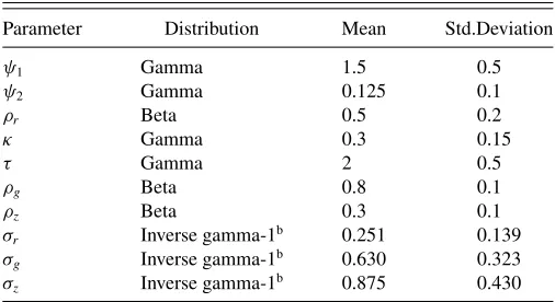
Table 1. Prior distributiona
Parameter Distribution Mean Std.Deviation
σr Inverse gamma-1b 0.251 0.139 σg Inverse gamma-1b 0.630 0.323 σz Inverse gamma-1b 0.875 0.430
NOTES:aThe inverse gamma-1 density is parameterized as in Bauwens, Lubrano, and
Richard (2000):ϕ(σ|ν,˜ s˜)= 2
Ŵ( ˜ν2)
s˜ 2
−2ν˜ σ−ν−˜ 1e−s/˜2σ2, where ˜ν=4 and ˜sequals 0.16,
1, and 1.96, respectively.
bFollowing DelNegro and Schorfheide (2004), we truncate the prior density such that the
parameter space is restricted to the determinacy region (corresponding to approximately 98.5% of the prior mass as defined above).
The shocksεz t,ε
g
t, and the monetary policy shock εtr are
as-sumed to be uncorrelated with each other and across time. Their standard deviation isσz,σg, andσr, respectively. The rational
expectations solution to the model can be calculated using var-ious methods, for example, Sims (2002). The model provides a complete description of comovement between output, inflation, and interest rates as a function of its deep parameters (denoted byθ, in what follows).
The prior distribution for θ is taken from DelNegro and Schorfheide (2004). Parameters are assumed to be indepen-dently distributed according toTable 1. We do not attempt to estimate the steady state values for the interest rate, and there-fore, calibraterγ∗ =β=0.99.
A central issue is to define the mappingZ, that is, to deter-mine how the economic concepts contained in the factors relate to the variables in the DSGE model. In our dataset, we include the measures of inflation, the growth rate of the output series, and the (nonannualized) interest rate series for our estimation. Therefore, we defineFDSGE
t =(y˜t,π˜t,r˜t)′, wherey˜t, ˜πt, and
˜
rtare the model implied equivalents of output growth, inflation,
and interest rates. WithSt =(yt, yt−1, πt, rt, zt, gt), the
map-ping from the DSGE model variables to the factors is
Z=
see DelNegro and Schorfheide (2004). The DSGE model equa-tions paired with the mappingZand the prior distribution forθ
allow the derivation of a prior distribution for the parameters in the state Equation (2) as described in Section3.2.
4.3 Prior for Observation Equation: Identification of Factors
The prior distribution on the coefficients in the observation equation induces the economic interpretation of the factors. The DSGE model contains the economic concepts “output growth,” “inflation,” and “short-term interest rates.” In the dataset, we have measures of these concepts as well as long-term interest
rates. Hence, we assume that a priori the output measures load exclusively on the first factor and the inflation series only on the second one. The short-term interest rates (with a maturity of at most one quarter) load solely on the third factor a priori, while the long-term interest rates load on all the factors. We set the corresponding element of0to one if a series loads on the
factor a priori, otherwise to zero. As for most of the series, we do not have a clear prior on the size of the loading, we impose only a rather flat prior by settingM0,n= 14IM in
n∼N0,n, RnM−0,n1
.
However, for three series, we do have a stronger prior: the GDP and its deflator are standard measures for output and prices and the FED funds rate is the most prominent measure for the short-term interest rate (see, e.g., Uhlig2005). For these series, we let the elements ofM0,nconverge to infinity, strictly
impos-ing that they exclusively load on their respective concept with the corresponding element of0,n equal to one and the other
elements of0,nequal to zero. In this case, Step 2 in Section3.3
reduces to settingn=0,nand drawingRnandnaccording
to the standard formulas with ¯Rn=s+u′nun. This identifies
the factors in the desired way, making it possible to interpret them as economic concepts. Note that these restrictions can be interpreted as exactly identifying restrictions for the factors in a classical framework. Hence, we rotate the factors in such a way that the standard measures for the variables in the DSGE model are directly and exclusively driven by the corresponding fac-tor. With respect to the remaining hyperparameters in the prior distribution, we sets=3 andν=4.001 to get a rather diffuse prior distribution with a finite variance (see Bauwens, Lubrano, and Richard2000, p. 303).
4.4 Implementation of the MCMC Algorithm
We iterateJ =500,000 times over Steps 1–3 described be-fore forλ∈(0.25,0.5,1,2,5,100). The lowest value forλis chosen such that the DSGE prior remains proper (see DelNegro and Schorfheide2004for a condition defining a threshold). The largest value,λ=100, corresponds to an almost strict imple-mentation of the DSGE model restrictions. To mitigate the effect of the initial values, set to values close to the prior mean, we discard the first 20% of the draws. For computational reasons, we evaluate only every 40th draw such that we have 10,000 draws to calculate the posterior distribution of the parameters.
We assess the convergence properties of the algorithm by running 10 distinct chains using different initial values, drawn from the prior distribution. Specifically, we drawθj fromϕ(θ)
allowing us to calculate(θj) and(θj), and then drawR,,
andfrom their prior distributions. Based on these chains, we compare between and within moments as proposed by Gelman and Rubin (1992) with the so-called scale reduction factor cal-culated as suggested by Brooks and Gelman (1998). Addition-ally, we rely on a number of graphical considerations including plots of recursively calculated moments and cusum path plots (see Yu and Mykland 1998). Gelman and Rubin (1992) sug-gested running the sampler until the squared scale reduction factor is below 1.2 or 1.1. For the structural hyperparameters
θ, the squared scale factor turned out to be below 1.1 after
ap-proximately 300,000. This somewhat slow convergence is due to chains with rather extreme initial draws. For the parameters that are relevant for forecasting, convergence is achieved much earlier, after approximately 50,000 draws. Therefore, we keep J =500,000 for the structural analysis, but setJ =250,000 in the forecasting exercise to reduce computational burden.
On a standard 1.2 GHz PC, around 160 min are needed to produce 100,000 draws. The exact time depends on the sample size and is also slightly influenced by the prior weightλ. The DSGE-based identification is calculated in less than a minute for 10,000 draws. For the sign-restriction approach, we draw 10 rotations for each draw of the posterior distribution, resulting in approximately 15,000 accepted draws. This procedure takes approximately 2 min on our 1.2 GHz PC.
The covariance matrix of the proposal draw is chosen propor-tionally to the dispersion of the prior distribution of each element ofθ, appropriately scaled to obtain an acceptance rate between 0.2 and 0.3. The degrees of freedom in thet-distribution of the proposal innovation is set to 40. The number of lagspin the state equation is 4. In the benchmark model, we replace the DSGE prior with a Minnesota-style prior. This is a natural benchmark, as it has been used by DelNegro and Schorfheide (2004) in the context of a Bayesian vector autoregression (BVAR), and has also been applied in the factor model literature (see, e.g., Kryshko2011). Further, by loosening the tightness of the prior, it approaches a classical likelihood-based model.
The Minnesota prior is implemented with dummy observa-tions as described in the appendix of Lubik and Schorfheide (2006). However, we adjust the parameters governing the first autoregressive coefficient to zero. The overall tightnessτ of the Minnesota-style prior is chosen by maximizing the marginal data density, resulting inτ =0.5, seeTable 3.
4.5 Forecast Performance
The analysis of the forecast performance suggests, first, that a positive but moderate weight of the DSGE prior is optimal and, second, that the DSGE-factor model improves the forecast as compared with a factor model with a nonstructural, Minnesota-style prior in some dimensions. These results are derived by comparing the forecasting performance during the last 10 years of the sample for different prior weightsλas follows. For each λand forecast horizonh, we calculate the covariance matrix of the forecast errors as
where Xt+h contains the standardized observed series and
PtXt+h is the corresponding forecast. Note thatPtXt+h is cal-culated based on newly estimated models using only data from 1985:1 totto mimic a real-time forecasting exercise. To mitigate the effect of occasional explosive roots, we calculatePtXt+has the median of the posterior distribution of forecasts. In addition to the models for different weightsλ, we estimate, for eacht, a benchmark model with a Minnesota-style prior as described in Section 4.4. Following DelNegro and Schorfheide (2004,
Table 2. Percentage gain in multivariate statistic (relative to forecast with Minnesota prior, bold values: maximum gain among
differentλ’s)
h/λ 0.25 0.5 1 2 3 5 100
Output
1 9 −0 0 0 1 −32 −36
4 5 0 0 0 −0 −35 −39
8 −2 −1 −1 −1 −1 −33 −36
12 1 1 1 1 2 −26 −36
Inflation
1 4 −2 −4 −4 −5 −66 −69
4 2 1 −0 −0 −1 −55 −60
8 −0 4 2 1 −0 −49 −50
12 −1 1 −0 −1 −3 −42 −47 Interest rate
1 35 22 26 30 29 −126 −131
4 32 17 22 29 27 −163 −166
8 29 18 21 22 20 −189 −184
12 30 19 20 24 21 −208 −207
see footnote 15 in their article), we calculate a multivariate statistic for the forecast performance as the converse of the log-determinant offorecastdivided by two times the dimension of
Xt. The percentage improvement of one model compared with
a benchmark model is calculated as the difference in the respec-tive statistic multiplied by 100. InTable 2, the percentage gain in the forecast precision of the factor model compared with the Minnesota-prior-based forecasts for the inflation, output, and interest rate series is documented. The results indicate that for horizons up to 1 year, the optimalλis small for all the series. However, for output and inflation, the optimal weight increases for longer horizons. Relative to the Minnesota-style prior, the performance is comparable for output and the inflation series. For interest rates, the performance of the DSGE-prior-based model is even better. We conclude that, overall, the DSGE-factor model performs well in terms of forecasting. While the optimal weight at short horizons is small, we find some evidence that more prior information helps at larger horizons. This finding is in line with the results obtained by DelNegro and Schorfheide (2004) with a DSGE-VAR for GDP, consumer price index (CPI) inflation, and the FED funds rate. The fact that the forecasting performance is improved in particular for interest rates under-lines a strength of our approach. The prior distribution includes a description of monetary policy that is widely regarded as a meaningful and fairly accurate. Hence, the results suggest that taking into account this prior information pays out in terms of forecasting performance.
4.6 In-Sample Fit
The analysis of the out-of-sample fit in the previous section narrowed the range of optimal weights to positive, but moderate values. This finding is confirmed and rendered more precisely by formally assessing the influence of the prior weight λ on the in-sample fit. Based on the posterior probabilities calcu-lated for λ∈(0.25,0.5,1,2,5,100), we are able to identify an optimal prior weight atλ=1. Thereby, we put equal prior
Table 3. Log-posterior marginal data density with Minnesota prior for varyingτ
q/τ 0.1 0.3 0.5 0.7 0.9
0.75 672 718 737 735 631
0.9 672 718 738 735 613
0.95 672 718 738 735 613
NOTE: Highest values printed in bold face.
weight on each model so that, in relative terms, only the pos-terior marginal data density pλ(X) is relevant. We calculate
this value by means of the modified harmonic mean estimator first proposed by Gelfand and Dey (1994) and implement this estimator following Geweke (1999). This method is readily im-plementable in our setting and the simulation exercise in Lopes and West (2004) suggests that the performance of this estimator in a factor model framework is not outperformed by other meth-ods investigated in that article. The prior distribution ϕ(j),
which needs to be evaluated to derive this estimator, can be cal-culated using the formulas in DelNegro and Schorfheide (2004) and Bauwens, Lubrano, and Richard (2000). The likelihood ϕ(X|j) is evaluated in closed form (see, e.g., Lopes and West
2004) by integrating out the factors with the Kalman filter. In Table 4, we see the log marginal data density for different weights of the DSGE priorλ. Two results emerge. First, we are able to identify an optimal prior weight atλ=1. Second, while the impact of marginal changes inλis moderate for small weights, the fit deteriorates for large values ofλ. Note that mag-nitude of the estimatedpλ(X) is to some extent influenced by
the choice of the “cut-off” valueq, determining which quan-tile of the draws is discarded for the harmonic mean estimator (see Geweke1999for a discussion). This is because the har-monic mean estimator ofpλ(X) can be sensitive to incidental
draws with an exceptionally low likelihood, introducing some numerical imprecision. However, the ranking of the models is invariant among different choices ofq. This supports that our conclusion is not affected by numerical imprecision. Some prior information from theory is useful, while strictly imposing the DSGE restrictions is clearly at odds with the data. The posterior marginal data density for the Minnesota prior is slightly higher, see Tables3and4. The fact that the Minnesota prior performs well in this respect is not surprising given that this prior is known to produce accurate forecasts and that posterior marginal data density equals the product of predictive likelihoods over the whole sample (see, e.g., Geweke2005, Corollary 2.6.1). Yet, given that the gain is only modest, we conclude that the advan-tages of our approach in other aspects, such as the structural interpretation, outweigh the slightly worse performance with regard to the posterior marginal data densities.
Table 4. Log-posterior marginal data density with DSGE prior for varyingλ
q/λ 0.25 0.5 1 2 3 5 100
0.75 536 609 733 727 713 −2251 −8547 0.9 371 609 734 728 713 −2251 −8547 0.95 372 609 734 728 713 −2251 −8547
NOTE: Highest values printed in bold face.
Table 5. Eighty percent HPD interval of DSGE model parameterθfor different weightsλ
λ 0.25 0.5 1 2 3 5 100
ψ1 [1.07 1.62] [1.05 1.58] [1.04 1.50] [1.06 1.54] [1.03 1.61] [1.30 1.98] [1.58 2.13] ψ2 [0.12 0.41] [0.14 0.47] [0.17 0.45] [0.19 0.55] [0.16 0.54] [0.09 0.53] [0.10 0.30] ρr [0.46 0.76] [0.53 0.77] [0.61 0.80] [0.63 0.81] [0.64 0.81] [0.65 0.81] [0.67 0.80]
κ [0.14 0.51] [0.14 0.45] [0.10 0.38] [0.09 0.34] [0.06 0.35] [0.03 0.17] [0.02 0.11]
τ−1 [1.49 2.70] [1.51 2.76] [1.80 3.17] [1.90 3.29] [2.02 3.45] [1.71 2.95] [1.54 2.89] ρg [0.84 0.95] [0.87 0.96] [0.91 0.97] [0.91 0.97] [0.93 0.98] [0.94 0.99] [0.95 0.99]
ρz [0.03 0.44] [0.07 0.49] [0.21 0.61] [0.33 0.71] [0.27 0.77] [0.72 0.99] [0.94 0.99]
σR [0.05 0.09] [0.05 0.10] [0.06 0.11] [0.06 0.11] [0.06 0.12] [0.03 0.10] [0.03 0.06]
σg [0.09 0.18] [0.08 0.16] [0.07 0.15] [0.06 0.15] [0.05 0.17] [0.09 0.33] [0.24 0.38]
σz [0.12 0.22] [0.14 0.23] [0.15 0.25] [0.15 0.25] [0.13 0.27] [0.07 0.18] [0.08 0.12]
4.7 Structural Analysis: The Impact of Monetary Policy Shocks
Measuring the impact of structural shocks hinges on different assumptions that disentangle causal relationships from correla-tions in the covariance matrix of the shocks. This is reflected
in the fact that we have to determine the rotation matrix(see Section3.4). The DSGE-based approach pins downrelying on the posterior distribution of the DSGE model, parameterized byθ. The highest posterior density (HPD) interval ofθfor dif-ferent weightsλis shown inTable 5. The coefficients forλ=1 are mostly similar to estimates in DelNegro and Schorfheide
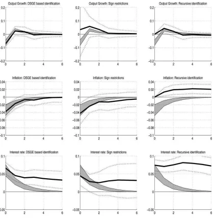
Figure 1. Response of output, inflation, and interest rate factor (first, second, third row, respectively) to a contractionary monetary shock: median and 80% HPD intervals (first column: DSGE-based identification, second column: sign-restriction-based identification, third column: recursive identification, gray shaded area: 80% HPD intervals of DSGE model implied responses).
Table 6. Eighty percent HPD intervals of factor loadings forλ=1
Output factor Inflation factor Interest rate factor
Disposable income [0.11 0.45] [−1.17−0.31] [0.05 0.40]
Final sales [0.23 0.64] [−1.68−0.70] [0.19 0.63]
GDP [1.00 1.00] [0.00 0.00] [0.00 0.00]
Gross national product (GNP) [0.61 0.99] [−1.29−0.40] [0.05 0.43]
National income [0.60 1.00] [−0.05 0.88] [−0.23 0.15]
Expenditures durables [−0.15 0.21] [−1.95−1.09] [0.10 0.52]
Expenditures total [0.08 0.49] [−2.16−1.20] [0.19 0.67]
Expenditures services [0.20 0.68] [−1.13 0.00] [0.12 0.59]
Expenditures nondurables [0.09 0.49] [−1.61−0.60] [−0.05 0.38] Industrial production index [1.20 1.58] [−0.31 0.34] [−0.19 0.16] Industrial production business equipment [0.84 1.27] [−0.28 0.60] [−0.14 0.31] Industrial production consumer goods [0.85 1.27] [−0.62 0.27] [−0.18 0.20] Industrial production durable consumer goods [0.85 1.36] [−0.93 0.08] [−0.24 0.23] Industrial production durable manufacturing [1.13 1.51] [−0.64 0.05] [−0.17 0.18] Industrial production durable materials [1.03 1.42] [−0.63 0.12] [−0.20 0.18] Industrial production final products [1.14 1.54] [−0.32 0.41] [−0.19 0.17] Industrial production manufacturing [1.22 1.60] [−0.44 0.18] [−0.16 0.17] Industrial production materials [1.07 1.47] [−0.39 0.32] [−0.23 0.15] Industrial production mining [0.25 0.73] [0.17 1.39] [−0.50 0.05] Industrial production nondurables goods [0.36 0.75] [−0.10 0.86] [−0.24 0.14] Industrial production nondurables manufacturing [0.85 1.28] [−0.11 0.88] [−0.32 0.13] Industrial production nondurable materials [0.82 1.27] [−0.32 0.71] [−0.27 0.23] Industrial production electric and gas utilities [0.03 0.38] [−0.32 0.61] [−0.17 0.18] Capacity utilization manufacturing [1.14 1.52] [−0.37 0.38] [−0.46 0.10] Capacity utilization [1.15 1.53] [−0.26 0.48] [−0.48 0.06] GDP chain-type price index [−0.14 0.12] [1.03 1.64] [−0.41−0.08]
GNP deflator [0.00 0.00] [1.00 1.00] [0.00 0.00]
GNP chain-type price index [−0.14 0.12] [1.03 1.64] [−0.40−0.07]
GDP deflator [−0.13 0.13] [1.05 1.65] [−0.40−0.07]
Private domestic investment chain-type price index [−0.14 0.11] [0.28 0.98] [−0.38 0.05] Consumer expenditure [−0.13 0.10] [0.31 0.95] [−0.12 0.27] Consumer expenditure less food [0.02 0.28] [1.15 1.70] [−0.37−0.05]
CPI [0.05 0.31] [1.12 1.67] [−0.38−0.06]
CPI apparel [0.05 0.30] [0.44 1.06] [−0.11 0.17]
CPI food and beverages [−0.16 0.10] [0.45 1.10] [−0.15 0.15] CPI other goods and beverages [−0.10 0.16] [−0.02 0.64] [0.05 0.35]
CPI housing [−0.15 0.10] [0.74 1.33] [−0.26 0.04]
CPI medical care [−0.13 0.08] [0.10 0.70] [−0.15 0.30]
CPI transportation [0.12 0.39] [0.83 1.45] [−0.49−0.18]
CPI urban consumers energy [0.08 0.36] [0.83 1.51] [−0.57−0.22] CPI urban consumers less energy [−0.10 0.13] [0.57 1.14] [−0.04 0.28] CPI urban consumers food [−0.13 0.13] [0.38 1.04] [−0.14 0.16] CPI urban consumers less food [0.06 0.33] [1.09 1.68] [−0.42−0.08] Moody’s Aaa corporate bond [0.05 0.27] [0.22 0.84] [0.25 0.78] Moody’s Baa corporate bond [0.04 0.25] [0.20 0.79] [0.22 0.74] 1 month certificate of deposit [−0.04 0.17] [0.01 0.60] [0.67 1.14] 3 month certificate of deposit [−0.02 0.20] [0.01 0.58] [0.69 1.14] 6 month certificate of deposit [0.03 0.27] [0.26 0.86] [0.69 1.12]
Federal funds rate [0.00 0.00] [0.00 0.00] [1.00 1.00]
1 year treasury constant maturity rate [0.07 0.30] [0.28 0.89] [0.70 1.11] 10 year treasury constant maturity rate [0.11 0.34] [0.24 0.86] [0.36 0.88] 2 year treasury constant maturity rate [0.11 0.34] [0.31 0.92] [0.66 1.07] 3 year treasury constant maturity rate [0.12 0.36] [0.28 0.91] [0.60 1.04] 3 month treasury constant maturity rate [−0.03 0.18] [0.05 0.63] [0.67 1.13] 5 year treasury constant maturity rate [0.12 0.36] [0.24 0.87] [0.49 0.98] 6 year treasury constant maturity rate [0.02 0.25] [0.28 0.88] [0.67 1.09] 7 year treasury constant maturity rate [0.12 0.35] [0.26 0.88] [0.44 0.96]
M2 own rate [−0.09 0.10] [−0.08 0.46] [0.35 0.86]
30 year mortgage rate [0.09 0.31] [0.14 0.76] [0.34 0.86]
Bank prime loan rate [−0.08 0.13] [0.02 0.62] [0.61 1.12]
Money Zero Maturity (MZM) own rate [−0.09 0.10] [−0.04 0.52] [0.38 0.90]
3 month treasury bill [−0.04 0.17] [0.04 0.62] [0.67 1.13]
6 month treasury bill [0.03 0.26] [0.29 0.89] [0.69 1.11]
Figure 2. Response of observed interest rates to a contractionary monetary shock: median and 80% HPD intervalsλ=1, FED funds rate (response identical toFigure 1) and Moodie’s Baa Bond (almost identical to Aaa Bond) omitted. Gray shaded area: response of interest rate factor, DSGE-based identification.
(2004). An exception is the reaction of the interest rate to ex-pected inflation in the Taylor rule (26), which is closer to one in our estimates. Note that this coefficient increases considerably with larger weightλ.
When implementing the alternative identification schemes, we follow standard procedures in the literature, but replace the observed variables with their corresponding factor. This results in a more robust identification with respect to idiosyncratic noise in observed variables. The recursive ordering is such that the output factor and inflation factor do not respond to monetary policy shocks contemporaneously following Boivin, Giannoni, and Mihov (2009). This assumption has been criticized on
var-ious grounds, for example, by Uhlig (2005). It may be reason-able to impose the timing restrictions in the setting of Boivin, Giannoni, and Mihov (2009) as they use monthly data. Clearly, the lower the data frequency, the less plausible is the assumption of no reaction within a period. In any case, our results show that this assumption is not innocuous.
In the sign-restriction approach, we impose that a contrac-tionary monetary policy shock does not lead to
• an increase in the price factor, • a decrease in the interest rate factor.
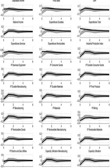
Figure 3. Response of observed output series to a contractionary monetary shock: median and 80% HPD intervalsλ=1, GDP omitted (response identical toFigure 1). Gray shaded area: response of interest rate factor, DSGE-based identification.
The restrictions are required to hold for the first two quar-ters, following Uhlig (2005) who restricted the responses in the first 5 months. We describe the results for the responses of the factors and the response of the observed series in the following paragraphs. In addition to the response ofFt-based
results based on the three different identification schemes, we report impulse responses ofFDSGE
t according to Equation (17).
We document all the results for our preferred prior weight λ=1.
4.7.1 Response of Common Factors. Generally, we find that the response of the factors based on the DSGE-based ap-proach resembles those implied by the standard New-Keynesian DSGE model (seeFigure 1): a contractionary monetary shock increases interest rates and has a negative impact on output
growth. The responses on impact in the factor model are close to the responses in the DSGE model. Hence, we do not ob-serve a “price puzzle”: a price increase following an unexpected monetary policy tightening. In some dimensions, there are also pronounced differences between the implications of the DSGE model and the factor model: one striking observation is that the reaction of interest rates to a monetary shock is far more persistent in the factor model than in the DSGE model.
Comparing the DSGE-based identification and the sign-restriction approach, we find that they do not lead to conflicting results: the 80% HPD based on the sign-restriction approach encompasses the intervals from the DGSE-based approach to a large extent. However, the intervals of the response on im-pact implied by the DSGE model rotation are more narrow than the intervals implied by the sign restriction. This is especially true for the reaction of the output factor. The sign-restriction approach produces an ambiguous sign of the response of out-put growth to a monetary policy shock on impact, in line with the results in Uhlig (2005). The DSGE-based approach, on the other hand, leads to a distinctively negative response. Hence, narrowing down the set of impulse responses based on restric-tions derived from theory removes much of the ambiguity of the response of output to monetary policy shocks.
While the responses derived with the DSGE-based iden-tification scheme confirms the predictions from theory to a large extent, this is not the case for a traditional Cholesky-decomposition-based identification scheme. The recursive or-dering provokes the so-called “price-puzzle,” rising prices as a response to a contractionary monetary policy shock.
4.7.2 Response of Observed Series. The factor model ap-proach allows for heterogenous responses of observed variables to shocks. Indeed, the observed variables do not move one to one with the factors, as documented by the 80% HPD intervals of the factor loadings inTable 6. Only the responses of GDP, the FED funds rate, and the GDP deflator are directly tied to the corresponding factor due to our identification restrictions for the factors.
The heterogeneity in the factor loadings directly translates into diverse effects of common shocks on observed variables. For the price variables, the loadings are mostly concentrated on the price factor. As a result, the response of observed prices is similar to the response of the price factor: prices decrease on impact, continue to fall modestly for up to another three quar-ters, and remain stable afterward. For short-term interest rates other than the FED funds rate, the reaction is slightly delayed as compared with the FED funds rate, but almost identical after one quarter (seeFigure 2). Hence, monetary policy shocks induce a broad-based change in short-term interest rates. As expected, the long-term interest rates react less on impact than the short-term interest rates, mainly due to their positive dependence on infla-tion. These results show that macroeconomic variables, such as output, have an additional impact on the long rates in addition to their impact through the “interest rate factor.” Hence, in our setup, the macroeconomic variables have an effect on the shape of the yield curve. This is consistent with results obtained by, for example, Diebold, Rudebusch, and Boragan Aruoba (2006). However, these authors found that changes in manufacturing capacity utilization—as a measure for output—are important determinants of the shape of the yield curve, but changes in
inflation are less important. We find that the term structure is in-fluenced by both current inflation and output. For output-related series, the responses are more heterogenous. While the response of industrial production in different sectors is similar to the re-sponse of the output factor, there are considerable deviations for other measures of output (Figure 3): disposable income and the consumption expenditures series increase moderately in re-sponse to a contractionary monetary policy shock. The size of the impact on consumption expenditure varies for different cate-gories. This finding is broadly in line with Boivin, Giannoni, and Mihov (2009), who found that there is a lot of variation in the response of personal consumption expenditures across different sectors but less variation in the corresponding price indicators.
5. CONCLUSION
Dynamic factor models are powerful tools for coping with large datasets. So far, theory and also applications focused mainly on finding statistically meaningful representations of the data. Inspired by the work of Boivin and Giannoni (2006) and DelNegro and Schorfheide (2004), we proposed a method to relate the statistical model to economic theory, without fully imposing the theoretical restrictions. Most importantly, the ex-plicit relationship to economic theory allows us to analyze the effect of policy interventions. We illustrated our method with an application on U.S. data and showed that a very simple New-Keynesian model proved to be useful for both forecasting and structural analysis.
Thus, with regard to a future research agenda, it seems to be worthwhile to apply the approach in other settings and with potentially less stylized models as theoretical background. A promising avenue for future research from a computational point of view is the application of a new generation of posterior simu-lators based on sequential Monte Carlo that are currently under development. On the one hand, as pointed out by Durham and Geweke (2012), sequential Monte Carlo allows to considerably reduce numerical errors in the estimation of the marginal data densities. On the other hand, these methods may open the door for the estimation of more complicated models, for example, models that are able to deal with nonlinear aspects of recent macroeconomic developments such as the conduct of monetary policy at the zero lower bound for nominal interest rates.
SUPPLEMENTARY MATERIAL
The supplementary material contains the definitions and sources of variables used in the empirical analysis, a detailed documentation of the test results regarding the number of factors in Section 4.1, and a description of the DSGE model leading to the log-linearized equations in Section 4.2.
ACKNOWLEDGMENTS
I thank two anonymous referees, Fabio Canova, Domenico Giannone, Marc Giannoni, Silvia Kaufmann, Klaus Neusser, Frank Schorfheide, Mark Watson, and Jonathan Wright for help-ful discussions and valuable comments. I also thank seminar participants at the Institute for Advanced Studies Vienna, the