Hybrid Genetic Algorithm and Simulated Annealing for Function Optimization

(1)

Journal Homepage: www.jitecs.ub.ac.id

Hybrid Genetic Algorithm and Simulated Annealing for

Function Optimization

Gusti Ahmad Fanshuri Alfarisy1_{, Andreas Nugroho Sihananto}2_{, Tirana Noor}

Fatyanosa3_{, M. Shochibul Burhan}4_{,Wayan Firdaus Mahmudy}5

Universitas Brawijaya, Faculty of Computer Science, Veteran Road. 8, 65145 Malang, Indonesia

1_{gusti.alfarisy@gmail.com,}2_{andreas.nugroho90@gmail.com,}3_{fatyanosa@gmail.com,} 4_{burhan.aan@gmail.com,}5_{wayanfm@ub.ac.id}

Received 9 Desember 2016; accepted 8 February 2017

Abstract. The optimization problems on real-world usually have non-linear characteristics. Solving non-non-linear problems is time-consuming. Thus heuristic approaches usually are being used to speed up the

solution’s searching. Among of the heuristic-based algorithms, Genetic

Algorithm (GA) and Simulated Annealing (SA) are two among most popular. The GA is powerful to get a nearly optimal solution on the broad searching area while SA is useful to looking for a solution in the narrow searching area. This study is comparing performance between GA, SA, and three types of Hybrid GA-SA to solve some non-linear optimization cases. The study shows that Hybrid GA-SA can enhance GA and SA to provide a better result.

1 Introduction

In recent years, Evolutionary Algorithm (EA) has already become an important tool to solve optimization problem such as multi-objective problems. This kind of problem sought to look for an optimal solution or nearest optimal solution to be achieved. However, sometimes that solution is hard to obtain if we use a common mathematical approach which may lead into local optimum only. To solve this kind of problems, we can use a heuristic algorithm such as Genetic Algorithm (GA) [1].

The genetic algorithm (GA) is a search algorithm that emulates the heredity and advancement of biology in a common habitat with the attributes of solid parallels, randomness, and self-adaption likelihood. The hypothetical establishments of the GA are the Darwinian biological evolution standard and Mendel's heredity hypothesis. The GA controls the search procedure utilizing existing data, merging to ideal or acceptable solutions by evaluating the fitness of chromosomes and also performing the selection, crossover, mutation and other genetic operations [2, 3].

(2)

adjustments. The solid is then gradually cooled in a controlled procedure until the solid crystallizes [5]. It is easy for SA to be modified, one of them is using functions or operators that are produced particularly according to the problem which used to generate the neighbor solution [6].

The SA can adequately escape local optima and meet to the global optima by joining a probabilistic hopping property with changing time qualities and an inclination to converge to zero in the inquiry procedure. The benefit of the GA and SA is that they are not restricted by the coherence or differentiability of the optimization issues. Thus, they are reasonable for complicated and nonlinear issues that conventional search strategies cannot solve. Nevertheless, the GA has poor nearby pursuit capacity, and the SA has low proficiency [7].

To overcome the both shortcomings of GA and SA, there are several studies proposed the hybrid between GA and SA. Junghans & Darde [5] compare between GA and hybrid GA with modified SA (MSA). The SA used in their experiment has been modified which control the reduction of the temperature. They found that hybrid GA-MSA provides higher reliability than GA.

Another research conducted by Chen & Shahandashti [8] which also compare the GA, SA, a hybrid of GA-SA, and MSA. They found that hybrid GA-SA is outperformed the GA, SA, and MSA. However, they ensure the fairness through the same total number of iterations, which is set to 10,000. This setting will lead to the unfairness as the GA is a population-based heuristics algorithm and SA is a non-population-based meta-heuristics algorithm.

In this paper, we hybrid the GA-SA with three scenarios, namely hybrid GA-SA, hybrid SA-GA, and cyclic GA-SA. The hybrid GA-SA process is to get the best solution in GA and use it as the initial population in SA. Otherwise, the hybrid SA-GA process is using the result from SA as the initial population for GA. While the cyclic GA-SA process is to randomly select the individual for interval 1000 iteration and improved by the SA, then processed again using GA.

2 Heuristic Algorithm

2.1 Genetic Algorithm (GA)

(3)

Start

Generate Initial Population

Calculate Fitness of Individuals

Satisfy stop criterion

Random Selection of parent

Extended Intermediate Crossover to produce children

Random Mutation of children

Calculate fitness of children

Elitism Selection to produce new

generation

End

No

Yes

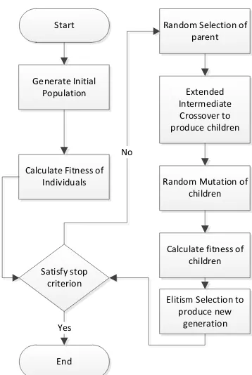
Fig. 1. The GA process

The GA will be processed some individuals, and they do crossover among individuals then mutate every child, result of the previous crossover. By calculating fitness among the children and the parents, the most ‘elite’ individual will be selected as new population, replace the old. This new population will be through crossover, mutation, and selection again until the stopping criteria met.

2.2 Simulated Annealing

Simulated Annealing is a local search algorithm that simulates the melting and cooling in metal processing. It has a variable initial temperature that set very high and gradually cooling by time to time[11]. Simulated Annealing usually implemented to search optimal solution on short range area even it sometimes also performs equally or even better than GA in some cases like research conducted by [12] to solve 8-Queens Problem or research by [13] that is looking for optimal reservoir operation by using GA and SA.

(4)

issue, the adjustment of the low vitality bonds at the warming stages is the fitness function of the optimization issue [5].

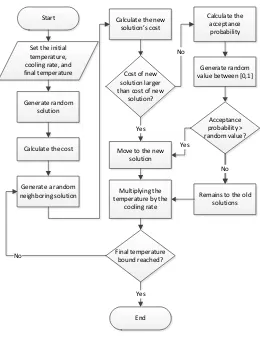
The controlled cooling procedure is the improvement procedure itself. In every emphasis step, the temperature is expected to diminish so that a low vitality obligation of the molecules is accepted. Inside the emphasis step, the algorithm seeks the neighbors of the present solution for a preferred arrangement. The iterative process is rehashed until a more proper arrangement is found [5]. The process of SA can be seen in Figure 2.

Start

Generate random solution Set the initial temperature, cooling rate, and final temperature

Calculate the cost

Generate a random neighboring solution

Calculate the new solution’s cost

Cost of new solution larger than cost of new

solution?

Move to the new solution

Calculate the acceptance probability

Generate random value between [0,1]

Acceptance probability > random value?

Remains to the old solutions Multiplying the

temperature by the cooling rate

Final temperature bound reached?

Yes

No

End Yes No

No

Yes

Fig. 2. The SA process

The SA is different from GA. SA have only one solution’s candidate and will be

(5)

2.3 Hybrid GA-SA

A hybrid between GA and SA may reach balanced the power of algorithms to let GA explore huge search of space and let SA exploit local search areas. While the standard SA typically begins with random initial parameter configuration of parameter settings, in the proposed solution, the best solution of the GA is utilized as the initial

configuration in SA.

This combination already studied by [14] which proved that Hybrid GA-SA outperforms common GA and SA. Another study by [15] shows that GA-SA hybrid can solve Permutation Flowshop Scheduling Problem.

Another research which utilizes local search-based algorithm conducted by [16]. The researchers implements hybridization between GA to explore huge search space and Variable Neighborhood Search (VNS) to exploit local search areas. They found that the hybridization delivers better outcomes comparable with the sequential approach.

For the sake of simplicity, we called this kind of hybridization as GASA1. The process of this hybrid method is starting by processing population on GA then processing the output of GA in SA to check whether the most optimal solution can be found. The process is being shown in Figure 3.

Start

Processed Through GA

Timeout for GA?

Select 50% best among last population

as SAs initial solution

Processed through SA

Timeout?

Output

Stop No

Yes

No

Yes

Fig. 3. Hybrid GA-SA process

(6)

2.4 Hybrid SA-GA

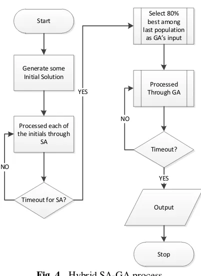
Almost same with hybrid GA-SA, hybrid SA-GA processing the input on SA first before continuing to GA. For the sake of simplicity, we called this kind of hybridization as GASA2. The process can be shown in Figure 4.

Start

Generate some Initial Solution

Processed each of the initials through

SA

Timeout for SA? NO

Processed Through GA

Timeout? Select 80% best among last population

as GA’s input

YES

Output

Stop YES NO

Fig. 4. Hybrid SA-GA process

To implement this hybrid, firstly we generate some initial population for SA. Then each of them will be handled by SA, and when they have been done, they will be GA’s initial population and addressed through GA until time allocation expiry.

2.5 Cyclic GA-SA

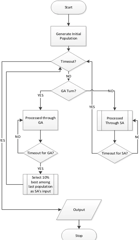
Another type of hybrid GA and SA is Cyclic GA-SA. For the sake of simplicity, we called this kind of hybridization as GASA3. This model will consist of some GA-SA iteration. On the first iteration, the input will be processed through GA first then some

of best GA’s output– 10% to be exact – will be processed in SA process. After that

(7)

Start

Processed through GA

Timeout for GA? NO

Processed Through SA

Timeout for SA?

Select 10% best among last population

as SA’s input YES

Output

Stop YES

NO Timeout?

NO

YES

GA Turn? YES

NO

Fig. 5. The Proses of Cyclic GA-SA

3 Experimental Result and Discussion

Besides using real-world problems, some papers also use test function. Test functions are artificial issues. It can be utilized to assess the conduct of an algorithm in some of the time various and troublesome circumstances [17]. Numerical experiments carried out by [18] shows that the evolved EA has better performance than the GA. They use unimodal and highly multimodal test function.

(8)

3.1 Experimental Scenario

We experiment with GA, SA, and hybridization of both algorithms which are GASA1, GASA2, and GASA3. All experimental algorithms were tested using five different test function which is described in Table 1.

Table 1. Test functions used in this study [19, 20]

Name Formula Range

Sphere (F1) 𝑓₀(𝑥⃗) = ∑ 𝑥_𝑖2

𝑛

𝑖=1

[−100,100]𝑛

Rosenbrock (F2)

𝑓1(𝑥⃗) = ∑(100(𝑥𝑖+1− 𝑥𝑖2)2

𝑛−1

𝑖=1

+ (𝑥𝑖− 1)2)

[−30,30]𝑛

Rastrigin (F3) 𝑓₂(𝑥⃗) = ∑(𝑥_𝑖2− 10 cos(2𝜋𝑥_𝑖) + 10)

𝑛

𝑖=1

[−5.12,5.12]𝑛

Cosine Mixture

(F4) 𝑓5(𝑥⃗) = ∑ 𝑥𝑖2− 0.1 ∑ cos⁡(5𝜋𝑥𝑖)

𝑛

𝑖=1 𝑛

𝑖=1

[−1,1]𝑛

Schwefel (F5) 𝑓₆(𝑥⃗) = 418.9829𝑛 − ∑ 𝑥_𝑖sin⁡(√|𝑥_𝑖|)

𝑛

𝑖=1

[−500,500]𝑛

In each testing scenario, we tune the different number of the random rate which is ranged between 0.1 and 1 to obtain the minimum value. We use random rate parameter to select the number of individual randomly that will be processed in GASA1, GASA2, and GASA3. The random rate of 0,1 in GASA1 means that the 10% of the population in GA will be addressed through SA while the random rate of 0,2 on GASA2 means that 20% of the number of individual SA will be dealt with through GA. While on the GASA3 random rate of 0,1 means only 10 % of the population that selected randomly will be put on GA then processed through SA and returned to GA.

For a fair comparison, we test all algorithm in the same environment. GA, SA, GASA1, GASA2, and GASA3 were coded in Scala programming language which provides both functional and object-oriented paradigm. This experiment uses multithreading concept. The first thread is working as a timer to stop the second thread that working as optimization process of each algorithm.

(9)

3.2 Result and Discussion

We conducted a test for 5 seconds and 60 seconds for all of the algorithms in ten attempts. The 5 seconds test is to analyze the best random rate for each algorithm in each function which will be used to analyze the 60 seconds computation time. The best random rate parameter for all hybrid algorithms in 5 seconds is described in detail in Table 2 – 4. It shows that on each test function, all hybrid algorithms have a different best parameter which is shown in bold type value.

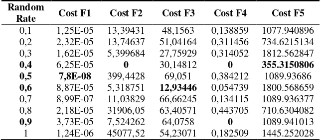
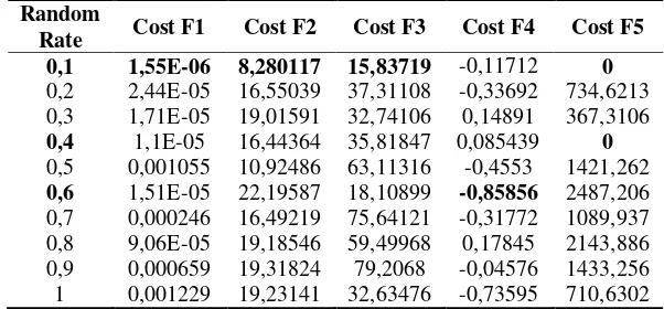
In GASA1, the best random rate for F2 and F5 is found on 0.4. While for F1 and F3, the best random rate is found on 0.5 and 0.6 respectively. For F4, the best random rates are 0.4 and 0.9. In GASA2, 0.8 is considered as the best random rate for F1 and F2. The best random rate for F4 is 0.1. The best random rates for F3 are 0.1 and 1.0. While for F5, the best random rates are 0.2, 0.8, and 0.9. In GASA3, test function of F1, F2, and F3 use 0.1 as the best random rate. For F4, 0.6 is found as the best random rate. For F5, the best random rates are 0.1 and 0.4. Furthermore, the summary of all best random rate is described in Table 5.

Even though each hybridization algorithm needs different random rate, they share the same behavior. In GASA1, about a half random rate is necessary to provide a better result. While in GASA2, the high number of random rate produce a better result. In GASA3, almost all of test function only need a low number of random rate.

Table 2. The GASA1’s random rate result

Random

Rate Cost F1 Cost F2 Cost F3 Cost F4 Cost F5

0,1 1,25E-05 13,39431 48,1563 0,138859 1077.940896

0,2 2,32E-05 13,74637 51,04164 0,311456 734.6215134

0,3 1,62E-05 5,399684 27,75929 0,314052 1812.562847

0,4 6,25E-05 0 30,14812 0 355.3150806

0,5 7,8E-08 399,4428 69,051 0,384212 1089.93686

0,6 8,87E-05 5,318751 12,93446 0,054739 1800.568659

0,7 8,99E-07 11,03829 66,66245 0,134115 1089.936377

0,8 2,18E-05 31906,05 63,40571 0,443705 710.6304082

0,9 3,73E-05 7,524262 64,0758 0 1089.941013

1 1,24E-06 45077,52 54,23071 0,182509 1445.252028

Random

0,1 1,78E-05 10,76142 0 -0,00437309 710,6302

0,2 6,72E-05 10,90107 26,76438 0,157753974 0

0,3 5,2E-05 6,184537 13,631 0 710,6306

0,4 0,000104 8,421549 15,72088 0 367,3107

(10)

0,6 7,75E-06 16,36613 15,02388 0,134492714 355,3151

Random

0,7 4,96E-05 13,90743 24,47611 0,069461259 355,3151

0,8 5,94E-06 5,559561 14,72731 0 0

0,9 8,43E-05 11,17417 15,22288 0,128197068 0

1 1,26E-05 11,04685 0 0,212436539 367,3106

Random

Rate Cost F1 Cost F2 Cost F3 Cost F4 Cost F5 0,1 1,55E-06 8,280117 15,83719 -0,11712 0

0,2 2,44E-05 16,55039 37,31108 -0,33692 734,6213

0,3 1,71E-05 19,01591 32,74106 0,14891 367,3106

0,4 1,1E-05 16,44364 35,81847 0,085439 0

0,5 0,001055 10,92486 63,11316 -0,4553 1421,262

0,6 1,51E-05 22,19587 18,10899 -0,85856 2487,206

0,7 0,000246 16,49219 75,64121 -0,31772 1089,937

0,8 9,06E-05 19,18546 59,49968 0,17845 2143,886

0,9 0,000659 19,31824 79,2068 -0,04576 1433,256

1 0,001229 19,23141 32,63476 -0,73595 710,6302

Table 5. Best random rate for GASA1, GASA2, and GASA3

Algorithm Best Random Rate

F1 F2 F3 F4 F5

GASA1 0.5 0.4 0.6 0.4/0.9 0.4

GASA2 0.8 0.8 0.1/1.0 0.1 0.2/0.8/0.9

GASA3 0.1 0.1 0.1 0.6 0.1/0.4

The best random rate for each algorithm in 5 seconds is used to test the best algorithm for each function in 60 seconds. The best algorithms for each benchmark functions in 60 seconds computation time described in detail in Table 6 – 11. It shows that on each test function has a different best algorithm with the different best random rate. The bold type value denotes the best value and the suffix “_0.1R” denotes random rate.

(11)

Table 6. The Comparison of Algorithms on the Sphere Function

Algorithm Average Min Max STD

SA 3.305274217 2.653319125 3.874782956 0.341572122

GA 1.13414E-06 0 1.12891E-05 3.56812E-06

GASA1_0.5R 1.97836E-06 0 1.50E-05 4.6456E-06

GASA2_0.8R 3.53527E-07 0 2.07157E-06 7.40544E-07

GASA3_0.1R 6.30704E-06 0 4.09383E-05 1.26652E-05

Min 3.53527E-07 0 2.07157E-06 7.40544E-07

Table 7. The Comparison of Algorithms on the Rosenbrock Function

SA 286.6908975 244.2679184 365.0979707 34.98299215

GA 19.61130637 0 35.69561389 13.81433565

GASA1_0.5R 10.64713993 0 27.23886208 13.74909805

GASA2_0.8R 10.89054876 0 27.74453831 14.06232146

GASA3_0.1R 10.90110841 0 27.59731668 14.07468841

Min 10.64713993 0 27.23886208 13.74909805

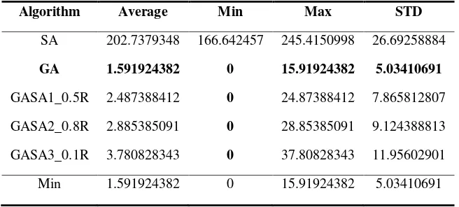
Table 8. The Comparison of Algorithms on the Rastrigin Function

SA 202.7379348 166.642457 245.4150998 26.69258884

GA 1.591924382 0 15.91924382 5.03410691

GASA1_0.5R 2.487388412 0 24.87388412 7.865812807

GASA2_0.8R 2.885385091 0 28.85385091 9.124388813

GASA3_0.1R 3.780828343 0 37.80828343 11.95602901

(12)

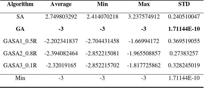
Table 9. The Comparison of Algorithms on the Cosine Mixture Function

SA 2.749803292 2.414070218 3.237574912 0.240510047

GA -3 -3 -3 1.71144E-10

GASA1_0.5R -2.202341837 -2.704431458 -1.66994172 0.369519055

GASA2_0.8R -2.394082464 -2.852215081 -1.965508857 0.27383257

GASA3_0.1R -2.32019165 -2.852215702 -1.817725862 0.328245019

Min -3 -3 -3 1.71144E-10

Table 10. The Comparison of Algorithms on the Schwefel Function

SA 6731.687029 5709.94333 8360.507287 771.8286095

GA 355.3150422 0 3553.150422 1123.60482

GASA1_0.5R 0 0 0 0

GASA2_0.8R 710.6300844 0 3553.150422 1498.13976

GASA3_0.1R 379.3061221 0 3793.061221 1199.471276

Min 0 0 0 0

From all tables, it can be concluded that generally, GA, GASA1 with a random rate of 0.5 and GASA2 with a random rate of 0.8 returned the best random rate for those functions. While SA produces the worst result for all function. The standard deviation for SA for each function consists of higher value than another algorithm. It shows that the result is widely spread which caused the obtained result is bad. The standard deviation for the best algorithm for each function consists of lower value which caused the obtained result is good.

4 Conclusion

(13)

rate which is sensitive with provided result. In the different case, random rate parameter needs to be tuned to obtain the best result.

References

1. Liu X, Jiao X, Li C, Huang M (2013) Research of Job-Shop Scheduling Problem Based on Improved Crossover Strategy Genetic Algorithm. In: Proc. 2013 3rd Int. Conf. Comput. Sci. Netw. Technol. pp 1–4

2. Mitchell M (1996) An introduction to genetic algorithms. MIT Press, Cambridge

3. Goldberg D (1989) Genetic algorithms in search, optimization and machine learning. Addison Wesley, New York

4. Kirkpatrick S, Gelatt CD, Vecchi MP (2007) Optimization by Simulated Annealing. Science (80- ) 220:671–680. doi: 10.1126/science.220.4598.671

5. Junghans L, Darde N (2015) Hybrid single objective genetic algorithm coupled with the simulated annealing optimization method for building optimization. Energy Build 86:651–662. doi: 10.1016/j.enbuild.2014.10.039

6. Mahmudy WF (2014) Improved simulated annealing for optimization of vehicle routing problem with time windows ( VRPTW ). Kursor 7:109–116.

7. Liu W, Ye J (2014) Collapse optimization for domes under earthquake using a genetic simulated annealing algorithm. J Constr Steel Res 97:59–68. doi: 10.1016/j.jcsr.2014.01.015

8. Chen PH, Shahandashti SM (2009) Hybrid of genetic algorithm and simulated annealing for multiple project scheduling with multiple resource constraints. Autom Constr 18:434–443. doi: 10.1016/j.autcon.2008.10.007

9. Deb K (2001) Multi-objective Optimization using Evolutionary Algorithms. Wiley, Chichester, United Kingdom

10. Vasan A (2005) Studies on advanced modeling techniques for optimal reservoir operation and performance evaluation of an irrigation system. Birla Institute of Technology and Science, Pilani, India

11. Brownlee J (2011) Clever Algorithms: Nature-Inspired Programming Recipes, 2nd ed.

12. Al-Khateeb B, Tareq WZ (2013) Solving 8-Queens Problem by Using Genetic Algorithms, Simulated Annealing, and Randomization Method. In: Int. Conf. Dev. eSystems Eng. pp 187–191

(14)

14. Crossland AF, Jones D, Wade NS (2014) Electrical Power and Energy Systems Planning the location and rating of distributed energy storage in LV networks using a genetic algorithm with simulated annealing. Int J Electr Power Energy Syst 59:103–110. doi: 10.1016/j.ijepes.2014.02.001

15. Czapinski M (2010) Parallel Simulated Annealing with Genetic Enhancement for flowshop problem. Comput Ind Eng 59:778–785. doi: 10.1016/j.cie.2010.08.003

16. Mahmudy W, Marian R, Luong L (2013) Hybrid Genetic Algorithms for Multi-Period Part Type Selection and Machine Loading Problems in Flexible

Manufacturing System. In: IEEE Int. Conf. Comput. Intell. Cybern. pp 126–130

17. Jamil M, Yang X-S (2013) A Literature Survey of Benchmark Functions For Global Optimization Problems Citation details: Momin Jamil and Xin-She Yang, A literature survey of benchmark functions for global optimization problems. Int

J Math Model Numer Optim 4:150–194. doi: 10.1504/IJMMNO.2013.055204

18. Oltean M (2003) Evolving Evolutionary Algorithms for Function Optimization. 7th Jt Conf Inf Sci 1:295–298.

19. Pehlivanoglu YV (2013) A New Particle Swarm Optimization Method Enhanced With a Periodic Mutation Strategy. 17:436–452.

20. Pant M, Thangaraj R, Abraham A (2009) Particle Swarm Optimization : Performance Tuning and Empirical Analysis. Foundations 3:101–128. doi: 10.1007/978-3-642-01085-9

Appendix: The experimental results details

Sphere Function

(15)

Ave-GASA3 0

Rosenbrock Function

Algorithm 1 2 3 4 5 6 7 8 9 10