CHAPTER 8
T Tests
A number of t tests are available, including: The One-Sample T Test
The Paired-Samples Test
The Independent-Samples T Test
8.1. One-Sample T Test
The One-Sample T Test procedure:
Tests the difference between a sample mean and a known or hypothesized value
Allows you to specify the level of confidence for the difference Produces a table of descriptive statistics for each test variable
8.1.1. A Production-Line Problem
A manufacturer of high-performance automobiles produces disc brakes that must measure 322 millimeters in diameter. Quality control randomly draws 16 discs made by each of eight production machines and measures their diameters.
This example uses the file brakes.sav. See the topic Sample Files for more information. Use One Sample T Test to determine whether or not the mean diameters of the brakes in each sample significantly differ from 322 millimeters.
8.1.1.1. Treating Each Machine as a Separate Sample
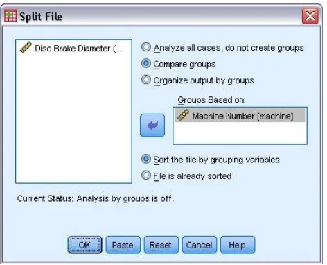
To split the file, from the Data Editor menus choose: Data > Split File...
Figure 101 Split File dialog box
1. Select Compare groups. 2. Select Machine Number. 3. Click OK.
8.1.1.2. Testing Sample Means against a Known Value
To begin the one-sample t test, from the menus choose: Analyze > Compare Means > One-Sample T Test...
Figure 102 One-Sample T Test dialog box
1. Select Disc Brake Diameter (mm) as the test variable. 2. Type 322 as the test value.
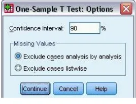
Figure 103 One-Sample T Test Options dialog box
4. Type 90 as the confidence interval percentage.
5. Click Continue.
6. Click OK in the One-Sample T Test dialog box.
8.1.1.3. Descriptive Statistics
Figure 104 Descriptive statistics, by Machine Number
8.1.1.4. Test Results
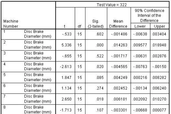
Figure 105 Test statistics, by Machine Number
The test statistic table shows the results of the one-sample t test.
The t column displays the observed t statistic for each sample, calculated as the ratio of the mean difference divided by the standard error of the sample mean.
The df column displays degrees of freedom. In this case, this equals the number of cases in each group minus 1.
The column labeled Sig. (2-tailed) displays a probability from the t distribution with 15 degrees of freedom. The value listed is the probability of obtaining an absolute value greater than or equal to the observed t statistic, if the difference between the sample mean and the test value is purely random.
The Mean Difference is obtained by subtracting the test value (322 in this example) from each sample mean.
Since their confidence intervals lie entirely above 0.0, you can safely say that machines 2, 5 and 7 are producing discs that are significantly wider than 322mm on the average. Similarly, because its confidence interval lies entirely below 0.0, machine 4 is producing discs that are not wide enough.
8.1.2. Summary
The one-sample t test can be used whenever sample means must be compared to a known test value. As with all t tests, the one-sample t test assumes that the data be reasonably normally distributed, especially with respect to skewness. Extreme or outlying values should be carefully checked; boxplots are very handy for this.
8.2. Paired-Samples T Test
One of the most common experimental designs is the "pre-post" design. A study of this type often consists of two measurements taken on the same subject, one before and one after the introduction of a treatment or a stimulus. The basic idea is simple. If the treatment had no effect, the average difference between the measurements is equal to 0 and the null hypothesis holds. On the other hand, if the treatment did have an effect (intended or unintended!), the average difference is not 0 and the null hypothesis is rejected.
The Paired-Samples T Test procedure is used to test the hypothesis of no difference between two variables. The data may consist of two measurements taken on the same subject or one measurement taken on a matched pair of subjects.
Additionally, the procedure produces:
Descriptive statistics for each test variable
A confidence interval for the average difference (95% or a value you specify)
8.2.1. Does Diet Make a Difference?
A physician is evaluating a new diet for her patients with a family history of heart disease. To test the effectiveness of this diet, 16 patients are placed on the diet for 6 months. Their weights and triglyceride levels are measured before and after the study, and the physician wants to know if either set of measurements has changed.
This example uses the file dietstudy.sav. See the topic Sample Files for more information. Use Paired-Samples T Test to determine whether there is a statistically significant difference between the pre- and post-diet weights and triglyceride levels of these patients.
8.2.1.1. Running the Analysis
To begin the analysis, from the menus choose:
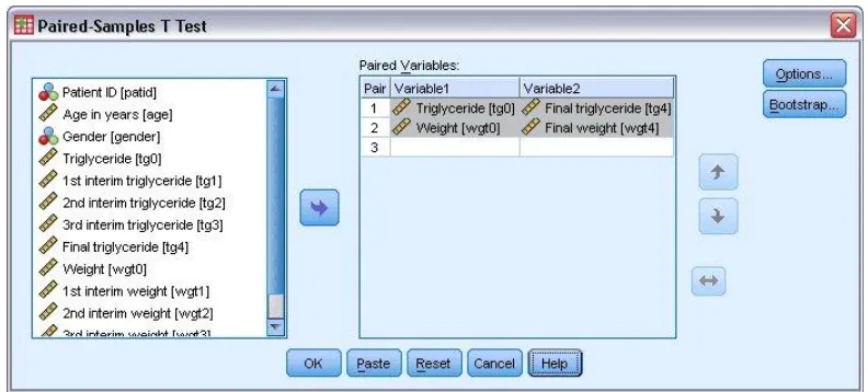
Analyze > Compare Means > Paired-Samples T Test... Figure 106 Paired-Samples T Test dialog box
1. Select Triglyceride and Final Triglyceride as the first set of paired variables.
8.2.1.2. Descriptive Statistics
The Descriptives table displays the mean, sample size, standard deviation, and standard error for both groups.
Across all 16 subjects, triglyceride levels dropped between 14 and 15 points on average after 6 months of the new diet.
The subjects clearly lost weight over the course of the study; on average, about 8 pounds.
The standard deviations for pre- and post-diet measurements reveal that subjects were more variable with respect to weight than to triglyceride levels.
8.2.1.3. Pearson Correlations
At -0.286, the correlation between the baseline and six-month triglyceride levels is not statistically significant. Levels were lower overall, but the change was inconsistent across subjects. Several lowered their levels, but several others either did not change or increased their levels.
On the other hand, the Pearson correlation between the baseline and six-month weight measurements is 0.996, almost a perfect correlation. Unlike the triglyceride levels, all subjects lost weight and did so quite consistently.
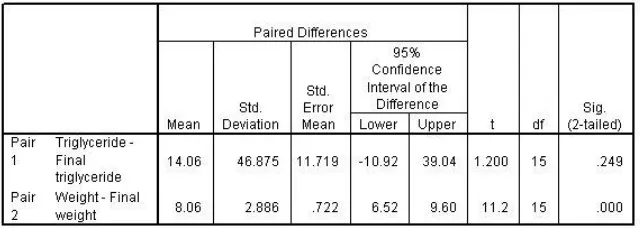
8.2.1.4. Paired Test Table
The Mean column in the paired-samples t test table displays the average difference between triglyceride and weight measurements before the diet and six months into the diet.
The Std. Deviation column displays the standard deviation of the average difference score.
The Std. Error Mean column provides an index of the variability one can expect in repeated random samples of 16 patients similar to the ones in this study.
The 95% Confidence Interval of the Difference provides an estimate of the boundaries between which the true mean difference lies in 95% of all possible random samples of 16 patients similar to the ones can conclude that the average loss of 8.06 pounds per patient is not due to chance variation, and can be attributed to the diet. However, the significance value greater than 0.10 for change in triglyceride level shows the diet did not significantly reduce their triglyceride levels.
8.2.2. Summary
Test variables with extreme or outlying values should be carefully checked; boxplots can be used for this.
If you compute the difference between the paired variables, you can alternatively use the One-Sample T Test procedure.
8.3. Independent-Samples T Test
The Independent-Samples T Test procedure tests the significance of the difference between two sample means. Also displayed are:
Descriptive statistics for each test variable A test of variance equality
A confidence interval for the difference between the two variables (95% or a value you specify)
8.3.1. Determining the Groups in an Independent-Samples T Test
Usually, the groups in a two-sample t test are fixed by design, and the grouping variable has one value for each group. However, there are times when assignment to one of two groups can be made on the basis of an existing scale variable. For example, consider math and verbal test scores. You would like to perform a t test on verbal scores, using the students above and below a given cutoff score on the math as the independent groups. With the Independent-Samples T Test procedure, all you need to provide is the cut point. The program divides the sample in two at the cut point and performs the t test. The virtue of this method is that the cut point can easily be changed without the need to re-create the grouping variable by hand every time.
8.3.2. Testing Two Independent Sample Means
received an ad promoting a reduced interest rate on purchases made over the next three months, and half received a standard seasonal ad. This example uses the file creditpromo.sav. See the topic Sample Files for more information. Use Independent-Samples T Test to compare the spending of the two groups.
8.3.2.1. Running the Analysis
To begin the analysis, from the menus choose:
Analyze > Compare Means > Independent-Samples T Test... Figure 108 Independent-Samples T Test dialog box
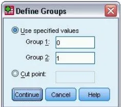
1. Select $ spent during promotional period as the test variable. 2. Select Type of mail insert received as the grouping variable. 3. Click Define Groups.
Figure 109 Define Groups dialog box
4. Type 0 as the Group 1 value and 1 as the Group 2 value.
5. Click Continue.
8.3.2.2. Group Statistics Table
Figure 110 Descriptive statistics
The Descriptives table displays the sample size, mean, standard deviation, and standard error for both groups. On average, customers who received the interest-rate promotion charged about $70 more than the comparison group, and they vary a little more around their average.
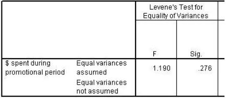
8.3.2.3. Independent Samples Test Table
Figure 111 Test for equality of group variances
The procedure produces two tests of the difference between the two groups. One test assumes that the variances of the two groups are equal. The Levene statistic tests this assumption. In this example, the significance value of the statistic is 0.276. Because this value is greater than 0.10, you can assume that the groups have equal variances and ignore the second test. Using the pivoting trays, you can change the default layout of the table so that only the "equal variances" test is displayed.
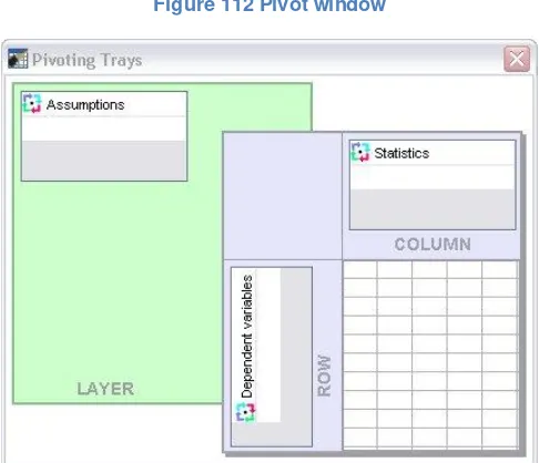
8.3.2.3.1. Pivoting the Test Table
1. Double-click the test table to activate it. 2. From the Viewer menus choose:
Figure 112 Pivot window
3. Move Assumptions from the row to the layer. 4. Close the pivoting trays window.
8.3.2.4. The Pivoted Test Table
Figure 113 t Test statistics, equal variances assumed
With the test table pivoted so that assumptions are in the layer, the Equal variances assumed panel is displayed.
The t column displays the observed t statistic for each sample, calculated as the ratio of the difference between sample means divided by the standard error of the difference.
The df column displays degrees of freedom. For the independent samples t test, this equals the total number of cases in both samples minus 2.
the probability of obtaining an absolute value greater than or equal
The 95% Confidence Interval of the Difference provides an estimate of the boundaries between which the true mean difference lies in 95% of all possible random samples of 500 cardholders.
Since the significance value of the test is less than 0.05, you can safely conclude that the average of 71.11 dollars more spent by cardholders receiving the reduced interest rate is not due to chance alone. The store will now consider extending the offer to all credit customers.
8.3.3. Using a Cut Point to Define the Samples
Churn propensity scores are applied to accounts at a cellular phone company. Ranging from 0 to 100, an account scoring 50 or above may be looking to change providers. A manager with 50 customers above the threshold randomly samples 200 below it, wanting to compare them on average minutes used per month.
This example uses the file cellular.sav. See the topic Sample Files for more information. Use Independent-Samples T Test to determine whether these groups have different levels of cell-phone usage.
8.3.3.1. Running the Analysis
To begin the analysis, from the menus choose:
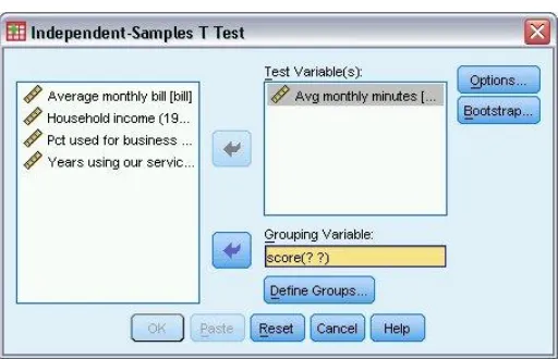
Figure 114 Independent-Samples T Test dialog box
1. Select Avg monthly minutes as the test variable. 2. Select Propensity to leave as the grouping variable. 3. Click Define Groups.
Figure 115 Define Groups dialog box
4. Select Cut point.
5. Type 50 as the cut point value.
6. Click Continue.
7. Click OK in the Independent-Samples T Test dialog box.
8.3.3.2. Group Statistics by Cut Point
Figure 116 Descriptive statistics, cellular-phone example
8.3.3.3. Test Table by Cut Point
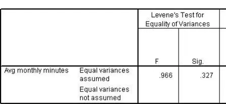
Figure 117 Test for equality of group variances
The significance value of the Levene statistic is greater than 0.10, so you can assume that the groups have equal variances and ignore the second test. Using the pivoting trays, change the default layout of the table so that only the "equal variances" test is displayed.
8.3.3.3.1. Pivoting the Test Table
1. Double-click the test table to activate it. 2. From the Viewer menus choose:
Pivot > Pivoting Trays
Figure 118 Pivot window
3. Move Assumptions from the row to the layer. 4. Close the pivoting trays window.
The t statistic provides strong evidence of a difference in monthly minutes between accounts more and less likely to change cellular providers.
The confidence interval suggests that in repeated samplings, the difference is unlikely to be much lower than 67 minutes. The company will look into ways to retain these accounts.
8.3.4. Summary
The independent-samples t test is appropriate whenever two means drawn from independent samples are to be compared. The variable used to form the groups may already exist; however, a cut point on a continuous variable can be provided to dynamically create the groups during the analysis. As with all t tests, the independent-samples t test assumes that each sample mean comes from a population that is reasonably normally distributed, especially with respect to skewness. Test variables with extreme or outlying values should be carefully checked; boxplots can be used for this.
CHAPTER 9
One-Way analysis of variance
You can use the One-Way ANOVA procedure to test the hypothesis that the means of two or more groups are not significantly different.
One-Way ANOVA also offers:
Group-level statistics for the dependent variable A test of variance equality
A plot of group means
Range tests, pairwise multiple comparisons, and contrasts, to describe the nature of the group differences
9.1. Testing the equality of group variances
An important first step in the analysis of variance is establishing the validity of assumptions. One assumption of ANOVA is that the variances of the groups are equivalent. This example illustrates how that test is performed.
A sales manager wishes to determine the optimal number of product training days needed for new employees. He has performance scores for three groups: employees with one, two, or three days of training. The data are in the filesalesperformance.sav. See the topic Sample Files for more information.
9.1.1. An error bar chart
Before running the analysis of variance, you graph the means and standard errors.
1. To create an error bar chart, from the menus choose: Graphs > Chart Builder...
4. Drag and drop Score on training exam onto the y axis.
5. Right-click Sales training group and select Nominal for the measurement level.
6. Drag and drop Sales training group onto the x axis. Figure 119 Simple error bar in Chart Builder
7. Click Element Properties.
Figure 120 Chart Builder, Element Properties
9. Click Apply and then click OK in the Chart Builder to create the error bar chart.
Average performance clearly increases with added training days, but variation in performance decreases at the same time. ANOVA assumes equality of variance across groups; that assumption may not hold for these data.
9.1.2. Running the analysis
To test the equality of variance assumption, from the menus choose: Analyze > Compare Means > One-Way ANOVA...
Figure 122 One-Way ANOVA dialog box
1. Select Score on training exam as the dependent variable. 2. Select Sales training group as the factor variable.
3. Click Options.
Figure 123 Options dialog box
6. Click OK in the One-Way ANOVA dialog box.
9.1.3. Descriptive statistics table
Figure 124 One-way ANOVA descriptive statistics table
The standard deviation and standard error statistics confirm that as training days increase, variation in performance decreases.
9.1.4. Levene test table
Figure 125 Homogeneity of variance table
The Levene statistic rejects the null hypothesis that the group variances are equal. ANOVA is robust to this violation when the groups are of equal or near equal size; however, you may choose to transform the data or perform a nonparametric test that does not require this assumption.
9.2. Performing a One-Way ANOVA
In response to customer requests, an electronics firm is developing a new DVD player. Using a prototype, the marketing team has collected focus group data. ANOVA is being used to discover if consumers of various ages rated the design differently.
This example uses the file dvdplayer.sav. See the topic Sample Files for more information.
9.2.1. Running the analysis
Figure 126 One-Way ANOVA dialog box
1. Select Total DVD assessment as the dependent variable. 2. Select Age Group as the factor variable.
3. Click Options.
Figure 127 Options dialog box
The means plot is a useful way to visualize the group differences. 4. Select Means plot.
5. Click Continue.
6. Click OK in the One-Way ANOVA dialog box.
9.2.2. ANOVA table
The significance value of the F test in the ANOVA table is less than 0.001. Thus, you must reject the hypothesis that average assessment scores are equal across age groups. Now that you know the groups differ in some way, you need to learn more about the structure of the differences.
9.2.3. A Plot of Group Means
Figure 129 One-Way ANOVA means plot
The means plot helps you to "see" this structure. Participants between the ages of 35 and 54 rated the DVD player more highly than their counterparts. If more detailed analyses are desired, then the team can use the range tests, pairwise comparisons, or contrast features in One-Way ANOVA.
9.3. Contrasts between means
Looking at the DVD data, market researchers ask:
Are the two groups between the ages of 35 and 54 really different from each other?
Can participants under 35 and over 54 be considered statistically equivalent?
This example uses the file dvdplayer.sav. See the topic Sample Files for more information.
9.3.1. Running the analysis
To begin the analysis, from the menus choose: Analyze > Compare Means > One-Way ANOVA...
Figure 130 One-Way ANOVA dialog box
1. Select Total DVD assessment as the dependent variable. 2. Select Age Group as the factor variable.
Figure 131 Contrasts dialog box, second contrast
The first contrast compares only groups 3 and 4; the others are eliminated by giving them weights of 0.
4. Enter the following contrast coefficients: 0, 0, -1, 1, 0, 0. Make sure to click Add after entering each value.
5. Click Next to move to the second contrast.
Figure 132 Contrasts dialog box, second contrast
6. Enter the following contrast coefficients: .5, .5, 0, 0, -.5, -.5. Make sure to click Add after entering each value.
7. Click Continue.
8. Click OK in the One-Way ANOVA dialog box.
9.3.2. Contrast coefficients table
Figure 133 One-Way ANOVA contrast-coefficient table
The contrast-coefficient table is a convenient way to check that the proper weights were given to the groups.
If the mean assessments of the DVD player for the 35-44 and 45-54 age groups are equal, then you would expect the observed difference in the mean assessment for these groups to be near 0. By specifying -1 and -1 as the contrast coefficients for these groups, the first contrast tests whether the observed difference is statistically significant.
Similarly, if the mean assessments of the under-35 age groups and over-54 age groups are equal, you would expect the sum of the first two groups to be equal to the sum of the last two groups, and the difference of these sums to be near 0.
9.3.3. Contrast test table
Figure 134 One-Way ANOVA contrast-test table
are unequal. In this case, the variances of the groups are assumed equal, so we focus on the first panel.
The significance values for the tests of the first contrast are both
9.4. All possible comparisons between means
Contrasts are an efficient, powerful method for comparing exactly the groups that you want to compare, using whatever contrast weights that you require. However, there are times when you do not have, or do not need, such specific comparisons. The One-Way ANOVA procedure allows you to compare every group mean against every other, a method known as pairwise multiple comparisons.
A sales manager has analyzed training data using One-Way ANOVA. While significant group differences were found, there are no prior hypotheses about how the three groups should differ. Therefore, he has decided to simply compare every group to every other group.
This example uses the file salesperformance.sav. See the topic Sample Files for more information.
9.4.1. Running the analysis
Figure 135 One-Way ANOVA dialog box
1. Select Score on training exam as the dependent variable. 2. Select Sales training group as the factor variable.
3. Click Post Hoc.
The Post Hoc tests are divided into two sets:
The first set assumes groups with equal variances.
The second set does not assume that the variances are equal. Because the Levene test has already established that the variances across training groups are significantly different, we select from this list.
4. Select Tamhane's T2. 5. Click Continue.
6. Click OK in the One-Way ANOVA dialog box.
9.4.2. Post hoc test table
The group with one training day performed significantly lower than the other groups.
Trainees with two and three days do not statistically differ in average performance. Despite this equality, the manager may still consider the added benefit of the third training day, given the large decrease in variability.
9.5. Summary
Validate the assumption of variance equality Obtain the ANOVA table and results
Visually inspect the group means
Perform custom contrasts, tailored to your specific hypotheses
Compare each mean to every other mean, assuming variance equality or not
Perform two types of robust analysis of variance
9.6. Related procedures
The One-Way ANOVA procedure is used to test the hypothesis that several sample means are equal.
You can alternately use the Means procedure to obtain a one-way analysis of variance with a test for linearity procedure.