Least Square Support Vector Machine: An Emerging Tool for Data Analysis
Palash Panja, Manas Pathak, Raul Velasco, and Milind Deo, University of Utah
Copyright 2016, Society of Petroleum Engineers
This paper was prepared for presentation at the SPE Low Perm Symposium held in Denver, Colorado, USA, 5– 6 May 2016.
This paper was selected for presentation by an SPE program committee following review of information contained in an abstract submitted by the author(s). Contents of the paper have not been reviewed by the Society of Petroleum Engineers and are subject to correction by the author(s). The material does not necessarily reflect any position of the Society of Petroleum Engineers, its officers, or members. Electronic reproduction, distribution, or storage of any part of this paper without the written consent of the Society of Petroleum Engineers is prohibited. Permission to reproduce in print is restricted to an abstract of not more than 300 words; illustrations may not be copied. The abstract must contain conspicuous acknowledgment of SPE copyright.
Abstract
Introduction
In the next five years the United States is expected to become the largest producer of oil in large part due to the production of liquids from tight oil reservoirs such as the Bakken or shales like the Eagle Ford. It is well recognized that ultra-low permeability reservoirs behave differently even when compared to low permeability reservoirs. Importance of the petrophysical parameters can be assessed using parameter sensitivity studies. Clear insight into the geologic and operational factors controlling production of oil/condensate and gas from these reservoirs was developed in this study using surrogate models.
The application of response surface method was started in the early nineties to find the optimal production and uncertainty associated with it (Damsleth et al., 1992,Egeland et al., 1992,Aanonsen et al., 1995). Effectiveness of RSM is thoroughly investigated by comparing various design of experiments (DOE) methods and different RSM (Yetenet al.,2005) and it is proved that response surface built through appropriate DOE is an efficient and fast proxy model for forecasting production performance and analyzing uncertainties (Amorim and Schiozer,2012). Amplitude factor and phase factors are adopted to separate out the highly non-linear effects from the remaining effects to forecast the oil rate and water cut (Li and Firedmann,2005). Among the artificial intelligence (AI) models, Artificial Neuron Networks (ANN) and Least Square Support Vector Machine (LSSVM) have become the most effective methods used in oil and gas industry. The RSM has been used for various purposes, these include estimating initial hydrocarbon uncertainty (Peng and Gupta,2003), finding an optimal scheme for well placements ( Guy-aguler and Horne,2001,Manceauet al.,2001,Manceau et al.,2002,Landa and Güyagüler,2003,Carreras
et al.,2006), uncertainty in production and recovery performance (Dejean and Blanc,1999,
Chewaroun-groajet al.,2000,Correet al.,2000,Venkataraman,2000,Manceauet al.,2001,Mohaghegh,2006), history matching (Landa and Güyagüler,2003, Yang et al.,2007, Slotte and Smorgrav,2008), and optimizing production to flow through nano-pores (Sarmaet al.,2005,Xieet al.,2013). The pressure and production are studied using field cases applying surrogate reservoir models which are based on pattern recognition techniques (Mohaghegh et al.,2012). AI was applied in unconventional fractured shale reservoirs ( Da-haghi et al.,2012, Xie et al.,2013) and tight reservoirs (Khosravi et al.,2011, Khosravi et al.,2012). Previous studies have shown that aquifer strength, fracture permeability and block height have a great impact on oil recovery (Khosravi et al.,2011) for low permeable fractured reservoirs. LSSVM approach is adopted more frequently over ANN for various purposes such as porosity and permeability determi-nation(Ammal F. Al-anazi,2010, Fatai Adesina Anifowose,2010, Fatai Adesina Anifowose,2011, Mo-hammad-Ali Ahmadi,2014), well placement(Mohammad-Ali Ahmadi,2015), water conning (Mohammad Ali Ahmadi,2014, Mohammad-Ali Ahmadi,2015) in horizontal wells, oil flow rate(Reza Gholgheysari Gorjaei,2015) and gas oil relative permeability(Ahmadi,2015). Support vector machines were also used to determine PVT properties such as bubble point pressure and formation volume factors of oil(E. El-Sebakhy,2007, Shahin Rafiee-Taghanaki,2013), constant volume depletion (CVD) behavior (Milad Arabloo,2014), dew point pressure(Mohammad Ali Ahmadi,2014,Arash Rabiei,2015), condensate to gas ratio (CGR) (Mohammad Ali Ahmadi,2014)of gas condensate system.
Methodology
Reservoir Model
A reservoir model with one horizontal well and a single vertical hydraulic fracture, located in the middle of the reservoir, was constructed for this study. The shape of the reservoir is taken as box shoe. The fracture height is considered the same as reservoir height. The reservoir dimensions in Y and Z directions are kept constant, and boundaries in the X-direction are varied. The matrix permeability, initial reservoir pressure and formation compressibility are varied. Fracture permeability, fracture width, fracture orientation, matrix porosity, initial hydrocarbon saturation and the reservoir temperature are kept constant. Parameters used in simulations are given in Table 1.
Input parameters
Selecting the important input parameters requires prior knowledge and experience of simulations for low permeability reservoirs. A mechanistic study(Palash Panja,2015) was conducted to choose the most significant petrophysical inputs and operating parameters. Eight factors, namely matrix permeability, gas relative permeability exponent, rock compressibility, initial gas oil ratio, slope of gas oil ratio in PVT, initial pressure, flowing bottom hole pressure and fracture spacing, are selected in this study. Depending on the type of DOE, each parameter may have different levels of values. The range of each variable is chosen based on observed data variability in specific fields, on completion data and on how each well operated as shown in Table 2.
Table 1—Simulation parameters used in the study.
Reservoir Top (ft.) 12000 Reservoir Thickness (ft.) 200 Reservoir Width (ft.) 750 Fracture Width (ft.) 0.05
Fracture Height (ft.) Reservoir Height Fracture Half length (ft.) Reservoir half width Fracture Orientation Parallel to YZ plane Reservoir Porosity (%) 5
Initial Water Saturation (%) 16
Number of grids Variable depending on Fracture spacing Minimum Size of grid (ft.) 0.05 (X-direction),3(Y-direction),3(Z-direction), Maximum size of grid(ft.) 6.5(X-direction), 110 (Y-direction), 20 (Z-direction),
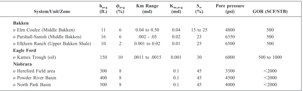
Table 2—Field data from various Shale plays (Chipman et. al, 2011)
System/Unit/Zone
o Elm Coulee (Middle Bakken) 11 6 0.04 to 0.50 0.04 15 to 25 4800 500 o Parshall-Sanish (Middle Bakken) 16 6 .002 - .05 0.02 23 6350 500 o Elkhorn Ranch (Upper Bakken Shale) 10 2 0.001 to 0.02 0.01 25 6500 500
Eagle Ford
o Karnes Trough (oil) 150 10 .0011 to .0015 0.001 30 6000 500 to 1000
Niobrara
o Hereford Field area 300 8 0.1 45 3500 ⬍2000
o Powder River Basin 400 8 0.1 45 4500 ⬍2000
In this study, only gas relative permeability exponent (ng) is varied, hence water-oil relative perme-abilities are fixed in all simulations.
Experimental Design
Many different designs of experiment techniques such as full factorial designs, fractional factorial designs, central composite design. The Box-Behnken (Box and Behnken,1960) DOE was determined to be best suited for this study to minimize the number of simulations for second order response surface model (RSM). According to the Box-Behnken technique, 114 simulations are designed for eight input parameters. The three absolute values of each input parameter except matrix permeability are scaled to
⫺1, 0 and⫹1 using a linear relationship. Logarithmic values of matrix permeability are also scaled using the same linear relationship. Ranges of all input parameters are summarized in Table 3.
In addition to 114 simulations, 30 simulations are designed from randomly chosen values of each input parameters. All input files are created for simulation using the combinations of independent variables prescribed by the Box-Behnken method and randomized procedure. Different combinations of input factors make each input file unique. The total number of input files is determined by the number of independent variables and by the design of the experiment method.
Surrogate Model
RSM and LSSVM are developed using total 144 simulation results after dividing the data randomly into training (80%) and test data (20%). We used the minimum number of grid blocks necessary to obtain converged results as we observed the sensitivity (Panja et al.,2013) of other parameters. All simulations were conducted using IMEX, a Computer Modeling Group Black-oil simulator. Two types of outcomes are investigated in this study, a time based model and a rate based model.
● In the time based model, outcomes (oil recovery, gas recovery and GOR) are recorded after certain
times such as 90 days, 1 year, 5 years, 10 years, 15 years and 20 years.
● In the rate based model, outcomes are obtained when the oil rate falls to 5 STB per day. Response Surface Model: 2nd order Polynomial
A second order model with first order variable interactions was chosen. The functional relationship of output with input variables are defined as:
(1)
Where,
Xi’s : the independent inputs
n : Total numbers of the independent inputs, n⫽8 for this study
Table 3—Ranges of input parameters chosen for the study Variable Symbol Minimum Maximum
1 Matrix Permeability, (nD) X1 10 5000 2 Gas Rel. Permeability Exponent, ng X2 1 3 3 Rock Compressibility, 1/psi X3 4⫻10-6 4
⫻10-5
4 dRs/dp, (SCF/STB)/psi X4 0.50 0.80 5 Initial Gas Oil Ratio, Rsi, SCF/STB X5 800 3000 6 Initial Pressure, Pi, psi X6 4000 6500
7 BHP, psi X7 500 1500
a0 : the intercept
ak’s and aij’s : the coefficients
僐 : Error term, Target variable (absolute value) in the multivariate method to minimize.
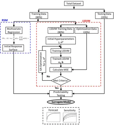
To avoid non-negative values of outcomes, regression was performed using logarithms of outcomes. The entire procedure of generating surrogate models (RSM and LSSVM) and its applications are shown in Figure 1.
Coefficients for all models of each outcome are produced using multivariate regressions by fitting the data in the second order model as displayed in Eq. 1 using Matlab (MathWorks® Inc.) programs where the residual term was minimized. Forty-five coefficients are obtained from each model. The model is then validated with the test data set to verify the robustness of the model. The surrogate models are then used for further study like forecasting and sensitivity analysis.
Least Square Support Vector Machines
The support vector machine (SVM), a part of machine learning field is a supervised learning technique. SVM is widely applied in classification and regression analysis. Many advantages of LSSVM over SVM
have encouraged researchers to apply this method to various fields. A brief description of theory of LSSVM is provided in Appendix B. Similar toequation 1, the following relationship is used in LSSVM (B.1)
The final form of LSSVM in linear relationship is given by equation B.8 as
(B.8)
K(x,xi) is called kernel function. Various kernel functions are given in theAppendix B. Selection of kernel function needs prior knowledge. Function can also be selected based on trial-error method. Radial Basis Function kernel is a good default kernel which demonstrates satisfactory results. Radial Kernel function is used in this study.
(B.9.3)
Regularization parameter,␥ and kernel parameter,␣2 in the LSSVM method are determined through optimization technique such as Genetic Algorithm (GA), Particle Swarm Optimization (PSO), and Simulated Annealing (SA) by minimizing the objective function. In this study, mean square error (MSE) (Equation A.2) between experimental (simulated) values and modeled values from LSSVM is considered as objective function with genetic algorithm (GA) optimization routine.
(A.2)
yexp and ymodel are the experimental and modeled values respectively.
The workflow for LSSVM is shown inFigure 1. LSSVM models are trained using Matlab toolbox (K. De Brabanter,2011) with 80% of training data, while 20% training data is used for optimization. The training data is split into two sets unlike RSM (where all training data are used for regression) because the predictability of the models is improved by avoiding overfitting of the models. The separate data set (20%) is utilized to seek the optimum values of ␥and ␣2
. To check this hypothesis, initially all training data were used to model LSSVM and to optimize ␥and ␣2
. The LSSVM models were almost perfectly fitted with experimental data (R2⬎1) but the predictability with the test data was adversely affected (R2⬎
0.7). Splitting the training data into 80%-20% gave optimum predictability performance. Trained LSSVM models (support values, iand bias term b) with optimized ␥ and ␣
2
are used for forecast and sensitivity analysis.
Results and Discussion
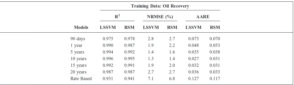
Oil recoveries, gas recoveries and gas oil ratio after 5 years, 10 years, 15 years, 20 years and when oil rate reaches minimum economic rate of 5 STB/day are generated by simulations. These data are used to create respective surrogate models, finally simulation and surrogate models (RSM and LSSVM) are cross plotted for compared to see the fitness. Goodness of model fit is quantitatively measured by calculating coefficient of determination, R2, Normalized Root Mean Square Error (NRMSE) and Average absolute relative error (AARE) (see Appendix A).
Acceptance of surrogate models is self-explanatory as shown in Figures 2a and b; both RSM and LSSVM models agree well with the simulation results. All recoveries fall well over the diagonal line. There are few variations between the simulations and the model. The measurement of fitness in terms of R2, NRMSE and AARE is provided in Table 4.
The coefficient of determination, R2, values indicate a good correlation between surrogate models and simulations. The coefficient of determination, R2, values are close to unity for time based models, and the data for the rate based model is slight scatter around the diagonal line with reasonably good value of R2. The predicted recoveries by model and the recoveries from simulation are in considerable agreement.
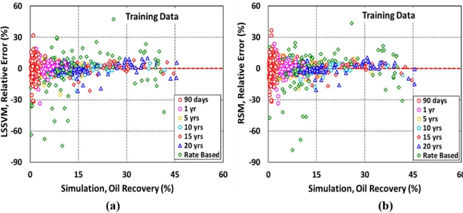
Deviation of models’ predictions are shown in Figure 3a & bin terms of relative error (seeAppendix A).
Figure 2—Fitness of models of oil recovery from training data for (a) LSSVM and (b) RSM
Table 4 —Fitness evaluation using statistical analysis of oil recovery models
Models
Training Data: Oil Recovery
R2 NRMSE (%) AARE
LSSVM RSM LSSVM RSM LSSVM RSM
Larger deviations are observed at the lower recovery values i.e., recovery obtained at initial time such as 90 days and 1 year. The economic rate of 5 STB/fracture/day also reaches very quickly even before first year of production. Rate based models predicts results with maximum errors (approximately ⫹50% to
⫺80%). The errors in time based models are in the range of a30%. R2and NRMSE for RSM and LSSVM models of oil recovery are compared in Figure 4a and b respectively.
It is evident that both RSM and LSSVM displayed a good fit with simulation results. The rate based models have poor performance as shown in lower R2 values (~0.935) and higher NRMSE (~7%).
Testing of the Surrogate Model
Validation of model through predictability using blind data set (test set) is an important part of model development. Surrogate models are generated based on the set of values of input factors as referred as training data. Models should be tested with the other values of input factors within the range of study.
Figure 3—Relative error distribution of oil recovery models using training data by (a) LSSVM (b) RSM
Unsatisfactory fit of models will prescribe the modifications in original models. In this study, the test (20% of all data) is kept aside to check model predictability. The modeled values are compared with simulations results using test data to demonstrate the robustness of the surrogate models. Oil recovery, gas recovery and gas oil ratio for time based models and rate based model are compared in Figures 5aand
b.
The overall fit of the models is satisfactory as indicated by R2 and NRMSE values (Table 5). Models of long term recoveries (after 5 years) are more accurate (R2⬎0.97 and NRMSE⬍7%) than the short term recovery models and rate based models. The relative error in oil recoveries are shown in Figure 6a and b.
Figure 5—Predictability of models of oil recovery from test data for (a) LSSVM and (b) RSM
Table 5—Predictability evaluation using statistical analysis of gas oil ratio models
Models
Test Data: Oil Recovery
R2 NRMSE (%) AARE
LSSVM RSM LSSVM RSM LSSVM RSM
Predictability of the surrogate model is satisfactory except the rate based models where ⫺125 % to
⫹50 aberrations are observed in low oil recoveries. The quantitatively errors are given in Table 5.
Forecast and Sensitivity Analysis
Forecast and sensitivity analysis are two of many applications of surrogate models. These applications are very rapid and easy to change the parameters. Any parameter or combination of parameters in the models can be varied deterministically or probabilistically for sensitivity analysis. Forecast of recovery at any time can be estimated from continuous recovery curves prepared by interpolating the available model data (90 days to 20 years) for intermediate time periods.
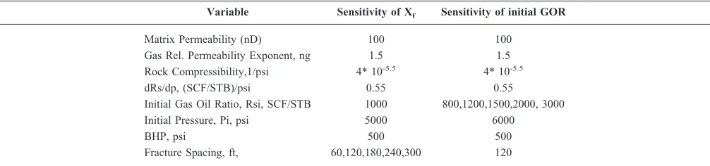
Sensitivities of fracture spacing and initial gas oil ratio on recovery are studied here. All other parameters except the parameter of interest are kept fixed as shown in Table 6.
The values of input parameters are chosen within the range of study. The results of sensitivity analysis are shown in Figure 8a and b.
Figure 6 —Relative error distribution of oil recovery models using training data by (a) LSSVM (b) RSM
Table 6 —Values of input parameters used in sensitivity studies Variable Sensitivity of Xf Sensitivity of initial GOR Matrix Permeability (nD) 100 100
Gas Rel. Permeability Exponent, ng 1.5 1.5 Rock Compressibility,1/psi 4* 10-5.5 4* 10-5.5
dRs/dp, (SCF/STB)/psi 0.55 0.55
Initial Gas Oil Ratio, Rsi, SCF/STB 1000 800,1200,1500,2000, 3000 Initial Pressure, Pi, psi 5000 6000
BHP, psi 500 500
No significant differences in oil recoveries predicted by LSSVM and RSM are observed. Only marginal difference in oil recoveries from LSSVM and RSM is noticed for initial gas oil ratio of 3000 SCF/STB as shown in Figure 8b. Low fracture spacing improves oil recovery as shown in Figure 8a. Major increase in recovery (approximately 8% at 20 years) is observed when fracture spacing is reduced from 120 feet to 60 feet. In case of low fracture spacing, most of oil in the reservoir portion is exploited and fracture interferes with the adjacent fractures. The stimulated volume is also reduced for low fracture spacing reservoir hence smaller reservoir volume is used in recovery factor calculation. The change in oil recovery is not significant (1-2% in 20 years) when fracture spacing increases beyond 180 feet. For ultra-low permeable reservoirs, fracture spacing of 180 feet seems to be very high. Transient state flow may persist for entire well life. Increasing fracture spacing increases the reservoir volume in calculation of recovery factor thus, for same amount of oil recovered during moving boundary transient state flow; recovery factor is less for higher fracture spacing. In Figure 6b, higher amount of oil is recovered with higher initial gas oil ratio. Higher initial gas oil ratio provides energy in reservoir to sustain pressure for long time. On the other hand, gas production is increased for higher initial gas oil ratio. Higher gas oil ratio helps production of oil by improving the oil mobility with dissolved gas
Conclusion
Surrogate reservoir models can be used for a quick assessment of production performance from ultra-low permeability reservoir like shales. Very few simulations are needed to generate the surrogate reservoir models. The methodologies to create various surrogate models (RSM and LSSVM) are demonstrated. Models are developed for different times (after 90 days, 1 year, 5 years, 10 years, 15 years and 20 years) and for a minimum economic rate (5 STB/ day). Eight factors, namely, matrix permeability, gas relative permeability exponent, rock compressibility, initial gas oil ratio, slope of gas oil ratio in PVT, initial pressure, flowing bottom hole pressure and fracture spacing, are selected to study the impacts on oil production from ultra-low permeable reservoirs. Both RSM and LSSVM exhibit good predictability to forecast the production such as oil recovery, gas recovery as surrogate models. The accuracy of the models is in the acceptance range. Thus the models for recoveries can be used confidently to predict the production for any input parameters value within the given ranges of study. The surrogate models of recoveries from ultra-low permeability reservoirs can be used confidently for any values of input factors within the range of study. These models are also useful to study the risk associated with the production
that will guide the development of a field. The support vector machine (SVM), a part of machine learning field is a supervised learning technique. Many advantages of LSSVM over SVM have encouraged researchers to apply this method to various fields. Least Square Support Vector Machine (LSSVM) is the most effective method for predictability over other AI methods such as Artificial Neuron Networks (ANN) because of its wide applicability to various aspects of reservoir engineering study.
References
1. Aanonsen, S.I., A.L. Eide, L. Holden and J.O. Aasen (1995). Optimizing Reservoir Performance Under Uncertainty with Application to Well Location. SPE Annual Technical Conference and Exhibition. Dallas, Texas, 1995 Copyright 1995, Society of Petroleum Engineers, Inc. SPE 30710.
2. Ahmadi, Mohammad Ali (2015).⬙Connectionist approach estimates gas– oil relative Connectionist approach estimates gas– oil relative simulation.⬙Fuel 140: 429 –439.
3. Amir Fayazi, Milad Arabloo, Amin Shokrollahi, Mohammad Hadi Zargari, Mohammad Hossein Ghazanfari (2014). ⬙State-of-the-Art Least Square Support Vector Machine Application for Accurate Determination of Natural Gas Viscosity.⬙Industrial & Engineering Chemistry Research 53: 945–958.
4. Ammal, F. Al-anazi, Gates, Ian D (2010).⬙Support-Vector Regression for Permeability Prediction in a Heterogeneous Reservoir: A Comparative Study.⬙SPE Reservoir Evaluation & Engineering13(03).
5. Amorim, Tiago C A De and Denis Jose Schiozer (2012). Risk Analysis Speed-Up With Surrogate Models. SPE Latin America and Caribbean Petroleum Engineering Conference. Mexico City, Mexico, Society of Petroleum Engineers. SPE153477s.
6. Arash Rabiei, Hossein Sayyad, Masoud Riazi, Abdolnabi Hashemi (2015).⬙Determination of dew point pressure in gas condensate reservoirs based on a hybrid neural genetic algorithm.⬙Fluid Phase Equilibria387: 38 –49.
Nomenclature
Symbol Description Units
a0 The intercept of the surrogate model
-ak Coefficient of independent input
-aij Coefficient of 2ndOrder Interaction of inputs
-BHP Bottom Hole Pressure psi
CGR Condensate to Gas Ratio STB/MMSCF dRs/dp Slope of gas/oil ratio in PVT (SCF/STB)/psi
GOR Gas/Oil Ratio SCF/STB
km Matrix Permeability nD
n Total numbers of independent inputs -ng Exponent of Relative Permeability Curve for Gas -NRMSE Normalized Root Mean Square Error -PDF Probability Density Function -Pi Initial Reservoir Pressure psi
PVT Pressure-Volume-Temperature
-qo Oil Rate STB/day
Rsi Initial Gas/Oil Ratio SCF/STB RMSE Root Mean Square Error Unit of Output R2 Coefficient of Determination
-SSres Residual Sum of Squares Unit of Output
SStot Total Sum of Squares Unit of Output
Xi Normalized Independent inputs
-Ymodel,i Modeled Value Unit of Output
Yobs,i Observed data Unit of Output
Yobs,max The Maximum value of Observed data Unit of Output
Yobs,min The Minimum value of Observed data Unit of Output
7. Box, G. E. P. and D. W. Behnken (1960).⬙Some New Three Level Designs for the Study of Quantitative Variables.⬙ Technometrics2(4): 455–475.
8. Carreras, Patricia Elva, Scott Edward Turner and Gwendolyn Tharp Wilkinson (2006). Tahiti: Development Strategy Assessment Using Design of Experiments and Response Surface Methods. SPE Western Regional/AAPG Pacific Section/GSA Cordilleran Section Joint Meeting. Anchorage, Alaska, USA, Society of Petroleum Engineers. 9. Chewaroungroaj, Jirawat, Omar, J. Varela and Larry, W. Lake (2000). An Evaluation of Procedures to Estimate
Uncertainty in Hydrocarbon Recovery Predictions. SPE Asia Pacific Conference on Integrated Modelling for Asset Management. Yokohama, Japan, Copyright 2000, Society of Petroleum Engineers Inc. SPE 59449.
10. Corinna Cortes, Vladimir Vapnik (1995).⬙Support-Vector Networks.⬙Machine Learning 20: 273–297.
11. Corre, B., P. Thore, V. de Feraudy and G. Vincent (2000). Integrated Uncertainty Assessment For Project Evaluation and Risk Analysis. SPE European Petroleum Conference. Paris, France, 2000,. Society of Petroleum Engineers Inc. SPE 65205.
12. Dahaghi, Amirmasoud Kalantari, Soodabeh Esmaili and Shahab, D. Mohaghegh (2012). Fast Track Analysis of Shale Numerical Models. SPE Canadian Unconventional Resources Conference. Calgary, Alberta, Canada, Society of Petroleum Engineers. SPE 162699.
13. Damsleth, Elvind, Asmund Hage and Rolf Volden (1992). ⬙Maximum Information at Minimum Cost: A North Sea Field Development Study With an Experimental Design.⬙Journal of Petroleum Technology44(12): 1350 –1356. 14. Dejean, J. P. and G. Blanc (1999). Managing Uncertainties on Production Predictions Using Integrated Statistical
Methods. SPE Annual Technical Conference and Exhibition. Houston, Texas, Society of Petroleum Engineers. SPE 56696.
15. E. El-Sebakhy, T. Sheltami, S. Al-Bokhitan, Y. Shaaban, I. Raharja, Y. Khaeruzzaman (2007). Support Vector Machines Framework for Predicting the PVT Properties of Crude-Oil Systems, Kingdom of Baharin, 15th SPE Middle East Oil & Gas Show and Conference.
16. Egeland, Thore, Lars Holden and E.A. Larsen (1992). Designing Better Decisions. European Petroleum Computer Conference. Stavanger, Norway, 1992 Copyright 1992, Society of Petroleum Engineers, Inc. SPE 24275.
17. Fatai Adesina Anifowose, AbdlAzeem Oyafemi Ewenla, Safiriyu Ijiyemi (2011). Prediction of Oil and Gas Reservoir Properties using Support Vector Machines, Bangkok, Thailand, International Petroleum Technology Conference,. 18. Fatai Adesina Anifowose, Abdulazeez Abdulraheem (2010). Prediction of Porosity and Permeability of Oil and Gas
Reservoirs using Hybrid Computational Intelligence Models, Cairo, Egypt, North Africa Technical Conference and Exhibition, SPE.
19. Guyaguler, Baris and Roland, N. Horne (2001). Uncertainty Assessment of Well Placement Optimization. SPE Annual Technical Conference and Exhibition. New Orleans, Louisiana, Copyright 2001, Society of Petroleum Engineers Inc. 20. Johan, A. K. Suykens, J. Vandewalle (1999).⬙Least Squares Support Vector Machine Classifiers.⬙Neural Processing
Letters9: 293–300.
21. Johan, A. K. Suykens, Tony Van Gestel, Jos De Brabanter, Bart De Moor, Joos Vandewalle (2002). Least Squares Support Vector Machines. Singapore, World Scientific Publishing Co. Pte. Ltd.
22. K. De Brabanter, P. Karsmakers, F. Ojeda, C. Alzate, J. De Brabanter, K. Pelckmans, B. De Moor, J. De Brabanter, K. Pelckmans, B. De Moor, (2011). LS-SVMlab Toolbox User’s Guide. Leuven, ESAT-SISTA Technical Report 10-146.
23. Khosravi, M., B. Rostami and S. Fatemi (2012). ⬙Uncertainty Analysis of a Fractured Reservoir’s Performance: A Case Study.⬙Oil Gas Sci. Technol. – Rev. IFP Energies nouvelles 67(3): 423–433.
24. Khosravi, Maryam, Shohreh Fatemi and Behzad Rostami (2011). Assessing Structured Uncertainty in a Mature Fractured Reservoir, Using Combination of Response Surface Method and Reservoir Simulation. SPE Reservoir Characterisation and Simulation Conference and Exhibition. Abu Dhabi, UAE, Society of Petroleum Engineers. SPE 148003.
25. Landa, Jorge, L. and Bars Güyagüler (2003). A Methodology for History Matching and the Assessment of Uncertainties Associated with Flow Prediction. SPE Annual Technical Conference and Exhibition. Denver, Colorado, Society of Petroleum Engineers. SPE 84465.
26. Li, Baoyan and Francois Firedmann (2005). A Novel Response Surface Methodology Based on⬙Amplitude Factor⬙ Analysis for Modeling Nonlinear Responses Caused by Both Reservoir and Controllable Factors. SPE Annual Technical Conference and Exhibition. Dallas, Texas, Society of Petroleum Engineers. SPE 95283.
28. Manceau, E., M. Mezghani, I. Zabalza-Mezghani and F. Roggero (2001). Combination of Experimental Design and Joint Modeling Methods for Quantifying the Risk Associated With Deterministic and Stochastic Uncertainties - An Integrated Test Study. SPE Annual Technical Conference and Exhibition. New Orleans, Louisiana, 2001,. Society of Petroleum Engineers Inc. SPE 71620.
29. Milad Arabloo, Shahin Rafiee-Taghanaki (2014).⬙SVM modeling of the constant volume depletion (CVD) behavior of gas condensate reservoir.⬙Journal of Natural Gas Science and Engineering21: 1148 –1155.
30. Mohaghegh, Shahab, D. (2006). Quantifying Uncertainties Associated With Reservoir Simulation Studies Using a Surrogate Reservoir Model. SPE Annual Technical Conference and Exhibition. San Antonio, Texas, USA, Society of Petroleum Engineers. SPE 102492.
31. Mohaghegh, Shahab, D., Jim S Liu, Razi Gaskari, Mohammad Maysami and Olugbenga A Olukoko (2012). Application of Well-Base Surrogate Reservoir Models (SRMs) to Two Offshore Fields in Saudi Arabia, Case Study. SPE Western Regional Meeting. Bakersfield, California, USA, Society of Petroleum Engineers. SPE 153845. 32. Mohammad-Ali Ahmadi, Alireza Bahadori (2015).⬙A LSSVM approach for determining well placement and conning
phenomena in horizontal wells.⬙Fuel153: 276 –283.
33. Mohammad-Ali Ahmadi, Mohammad Reza Ahmadi, Seyed Moein Hosseini, Mohammad Ebadi (2014). ⬙ Connec-tionist model predicts the porosity and permeability of petroleum reservoirs by means of petro-physical logs: Application of artificial intelligence.⬙Journal of Petroleum Science and Engineering 123: 183–200.
34. Mohammad Ali Ahmadi, Reza Soleimani, Moonyong Lee, Tomoaki Kashiwao, Alireza Bahadori (2015).⬙ Determi-nation of oil well production performance using artificial neural network (ANN) linked to the particle swarm optimization (PSO) tool.⬙Petroleum.
35. Mohammad Ali Ahmadi, Mohammad Ebadi (2014).⬙Evolving smart approach for determination dew point pressure through condensate gas reservoirs.⬙Fuel117: 1074 –1084.
36. Mohammad Ali Ahmadi, Mohammad Ebadi, Payam Soleimani Marghmaleki, Mohammad Mahboubi Fouladi (2014). ⬙Evolving predictive model to determine condensate-to-gas ratio in retrograded condensate gas reservoirs.⬙Fuel124: 241–257.
37. Mohammad Ali Ahmadi, Mohammad Ebadi, Seyed Moein Hosseini (2014).⬙Prediction breakthrough time of water coning in the fractured reservoirs by implementing low parameter support vector machine approach.⬙ Fuel 117: 579 –589.
38. Palash Panja, Tyler Conner, Milind Deo (2015). ⬙Factors Controlling Production in Hydraulically Fractured Low Permeability Oil Reservoirs.⬙International Journal of Oil, Gas and Coal Technology.
39. Panja, Palash, Tyler Conner and Milind Deo (2013). ⬙Grid sensitivity studies in hydraulically fractured low permeability reservoirs.⬙Journal of Petroleum Science and Engineering112(0): 78 –87.
40. Peng, Cheong Yaw and Ritu Gupta (2003). Experimental Design in Deterministic Modelling: Assessing Significant Uncertainties. SPE Asia Pacific Oil and Gas Conference and Exhibition. Jakarta, Indonesia, Society of Petroleum Engineers. SPE 80537.
41. Reza Gholgheysari Gorjaei, Reza Songolzadeh, Mohammad Torkaman, Mohsen Safari, Ghassem Zargar (2015). ⬙A novel PSO-LSSVM model for predicting liquid rate of two phase flow through wellhead chokes.⬙Journal of Natural Gas Science and Engineering24: 228 –237.
42. Sarma, Pallav, Louis J Durlofsky and Khalid Aziz (2005). Efficient Closed-loop Production Optimization Under Uncertainty. SPE Europec/EAGE Annual Conference. Madrid, Spain, Society of Petroleum Engineers. SPE 94241. 43. Shahin Rafiee-Taghanaki, Milad Arabloo, Ali Chamkalani, Mahmood Amani, Mohammad Hadi Zargari, Mohammad Reza Adelzadeh (2013).⬙Implementation of SVM framework to estimate PVT properties of reservoir oil.⬙Fluid Phase Equilibria346: 25–32.
44. Slotte, Per Arne and Eivind Smorgrav (2008). Response Surface Methodology Approach for History Matching and Uncertainty Assessment of Reservoir Simulation Models. Europec/EAGE Conference and Exhibition. Rome, Italy, Society of Petroleum Engineers. SPE 113390.
45. Venkataraman, R. (2000). Application of the Method of Experimental Design to Quantify Uncertainty in Production Profiles. SPE Asia Pacific Conference on Integrated Modelling for Asset Management. Yokohama, Japan, Copyright 2000, Society of Petroleum Engineers Inc. SPE 59422.
46. Xie, Jiang, Seong Lee, Xian-huan Wen and Zhiming Wang (2013). Uncertainty Assessment of Production Perfor-mance for Shale Gas Reservoirs. 6th International Petroleum Technology Conference. Beijing, China, 2013, Inter-national Petroleum Technology Conference. IPTC 16866.
Appendix A
Goodness of Fit
There are many statistical tests to measure the accuracy or goodness of a modeled curve. R-squared (R2) and normalized root mean squared error, relative error, and absolute average relative error are used in this study to evaluate the regression models.
The coefficient of determination (R
2):
The coefficient of determination, R2, indicates the overall accuracy of a regression. The R2, is defined as:
(A1)
Where,
, the residual sum of squares , the total sum of squares
, the mean of observed values
The values of R2range from 0 to 1. The values closed to unity are interpreted as the better fit of the model curve with observed data.
Normalized Root Mean Square Error (NRMSE):
(A.2)
The Root Mean Square Error (RMSE) (also known as the root mean square deviation, RMSD), is used to measure the total residuals of modeled values and observed values.
The RMSE is defined as the square root of the mean squared error:
(A.3)
Where Yobsis observed values and Ymodel is modeled values.
Sometimes, it is difficult to analyze the error in terms of absolute values because different outcomes vary in their absolute values, ranges and units. Non-dimensional forms of the RMSE are required to compare RMSE for different units and outcomes. The RMSE is normalized by dividing with the range of the observed data to get NRMSE (Normalized Root Mean Square Error) as follows:
(A.4)
Where,
Yobs,max is the maximum value of observed data. Yobs,min is the minimum value of observed data.
The NRMSE can be expressed in term of percentage by multiplying by 100. The smaller percentage values indicate the better fit of the model curve with observed data.
Average absolute relative error (AARE)
Relative error is measured for a particular point asThis the direct measurement of total relative errors. Absolute values of errors are generally used to prevent the nullification of errors when adding positive and negative deviations. Another feature of AARE is that it does not consider absolute value of errors but calculates error relative to the actual value. The calculation method is shown in Equation A4
Appendix B
Theory of Least Square Support Vector Machine
The LSSVM is developed by Suykens et al.(Johan A. K. Suykens,1999, Johan A. K. Suykens,2002) by changing the inequality constraints in traditional support vector machines (SVM)(Corinna Cortes,1995). The mathematical background is discussed in numerous places, a summary is given here. The regression model from given training data (of size N) for LSSVM is given in equation B.1.
(B.1)
Where (x) is the nonlinear mapping function and w and b are the weight vector and bias term, respectively which are determined by linear regression formulated as equation B.2.
(B.2)
Subject to
(B.3)
where ␥ is the regularization parameter to prevent over fitting. The term ei is the model error. To solve the restricted optimization problem given inequation B.2, first it is turned into unrestricted by Lagrange multipliers (di), then optimal situation is found by partial derivatives based on the Karush-Kuhn-Tucker (KKT). Detailed calculations are given by Suyken et al.(Johan A. K. Suykens,1999,Johan A. K. Suykens,2002,Amir Fayazi,2014,Mohammad Ali Ahmadi,2015).
(B.4)
Where,
Values of b and V are obtained after solving equation B.4
(B.5)
(B.6)
Final form of LSSVM i.e. equation B.1 after applying Mercer’s theorem is given as
(B.7)
where ⍀ij ⫽ (xi)T (x
j) ⫽ K(xi, xj). Values of b and ␣ can be calculated by replacing ⍀ by K in
K(x,xi) is kernel function. Various kernel functions are discussed in next section. Linear relationship given in equation B.4 can be described as
(B.8)
Kernel Function
Various kernel functions that satisfy Mercer’s condition are available such as linear, polynomial, radial basis function (also known as Gaussian), exponential, Laplacian, hyperbolic tangent (also known as sigmoid and Multilayer Perceptron (MLP)) etc.
(B.9.1)
(B.9.2)
(B.9.3)
(B.9.4)
Using RBF,equation 7 becomes
(B.10)
x and xi are vectors of size p (number of parameters)
Expanding equation 10
Appendix C
Gas Recovery and Gas Oil Ratio
Figure C.1—Fitness of models of gas recovery from training data for (a) LSSVM and (b) RSM
Table C.1—Fitness evaluation using statistical analysis of gas recovery models
Models
Training Data: Gas Recovery
R2 NRMSE (%) AARE
LSSVM RSM LSSVM RSM LSSVM RSM
Figure C.2—Predictability of models of gas recovery from test data for (a) LSSVM and (b) RSM
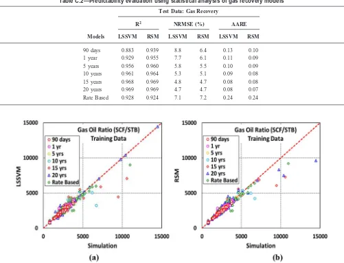
Table C.2—Predictability evaluation using statistical analysis of gas recovery models
Models
Test Data: Gas Recovery
R2 NRMSE (%) AARE
LSSVM RSM LSSVM RSM LSSVM RSM
90 days 0.883 0.939 8.8 6.4 0.13 0.10 1 year 0.929 0.955 7.7 6.1 0.11 0.09 5 years 0.956 0.960 5.8 5.5 0.10 0.09 10 years 0.961 0.964 5.3 5.1 0.09 0.08 15 years 0.968 0.969 4.8 4.7 0.08 0.08 20 years 0.969 0.969 4.7 4.7 0.08 0.07 Rate Based 0.928 0.924 7.1 7.2 0.24 0.24
Table C.3—Fitness evaluation using statistical analysis of gas oil ratio models
Models
Training Data: Gas Oil Ratio
R2 NRMSE (%) AARE
LSSVM RSM LSSVM RSM LSSVM RSM
90 days 0.977 0.979 3.1 2.9 0.03 0.03 1 year 0.966 0.973 3.8 3.4 0.03 0.03 5 years 0.969 0.974 3.5 3.2 0.04 0.04 10 years 0.823 0.895 6.7 5.2 0.07 0.06 15 years 0.769 0.864 6.7 5.1 0.09 0.07 20 years 0.989 0.882 1.4 4.5 0.03 0.08 Rate Based 0.938 0.947 3.5 3.2 0.08 0.07
Figure C.3—Predictability of models of gas oil ratio from test data for (a) LSSVM and (b) RSM
Table C.4 —Predictability evaluation using statistical analysis of gas oil ratio models
Models
Test Data: Gas Oil Ratio
R2 NRMSE (%) AARE
LSSVM RSM LSSVM RSM LSSVM RSM