Micha Gorelick & Ian Ozsvald
High Performance
Python
PR ACTICAL PERFORMANT
PROGR AMMING FOR HUMANS
PY THON / PERFORMANCE Your Python code may run correctly, but you need it to run faster. By
exploring the fundamental theory behind design choices, this practical guide helps you gain a deeper understanding of Python’s implementation. You’ll learn how to locate performance bottlenecks and significantly speed up your code in high-data-volume programs.
How can you take advantage of multi-core architectures or clusters? Or build a system that can scale up and down without losing reliability? Experienced Python programmers will learn concrete solutions to these and other issues, along with war stories from companies that use high performance Python for social media analytics, productionized machine learning, and other situations.
■ Get a better grasp of numpy, Cython, and profilers ■ Learn how Python abstracts the underlying computer
architecture
■ Use profiling to find bottlenecks in CPU time and memory usage ■ Write efficient programs by choosing appropriate data
structures
■ Speed up matrix and vector computations
■ Use tools to compile Python down to machine code
■ Manage multiple I/O and computational operations concurrently ■ Convert multiprocessing code to run on a local or remote cluster ■ Solve large problems while using less RAM
Micha Gorelick, winner of the Nobel Prize in 2046 for his contributions to time
travel, went back to the 2000s to study astrophysics, work on data at bitly, and co-found Fast Forward Labs as resident Mad Scientist, working on issues from machine learning to performant stream algorithms.
Ian Ozsvald is a data scientist and teacher at ModelInsight.io, with over ten years
Micha Gorelick and Ian Ozsvald
High Performance Python
High Performance Python
by Micha Gorelick and Ian Ozsvald
Copyright © 2014 Micha Gorelick and Ian Ozsvald. All rights reserved. Printed in the United States of America.
Published by O’Reilly Media, Inc., 1005 Gravenstein Highway North, Sebastopol, CA 95472.
O’Reilly books may be purchased for educational, business, or sales promotional use. Online editions are also available for most titles (http://safaribooksonline.com/). For more information, contact our corporate/ institutional sales department: 800-998-9938 or [email protected].
Editors: Meghan Blanchette and Rachel Roumeliotis
Production Editor: Matthew Hacker
Copyeditor: Rachel Head
Proofreader: Rachel Monaghan
Indexer: Wendy Catalano
Cover Designer: Karen Montgomery
Interior Designer: David Futato
Illustrator: Rebecca Demarest September 2014: First Edition
Revision History for the First Edition:
2014-08-21: First release
See http://oreilly.com/catalog/errata.csp?isbn=9781449361594 for release details.
Nutshell Handbook, the Nutshell Handbook logo, and the O’Reilly logo are registered trademarks of O’Reilly Media, Inc. High Performance Python, the image of a fer-de-lance, and related trade dress are trademarks of O’Reilly Media, Inc.
Many of the designations used by manufacturers and sellers to distinguish their products are claimed as trademarks. Where those designations appear in this book, and O’Reilly Media, Inc. was aware of a trademark claim, the designations have been printed in caps or initial caps.
While every precaution has been taken in the preparation of this book, the publisher and authors assume no responsibility for errors or omissions, or for damages resulting from the use of the information contained herein.
Table of Contents
Preface. . . ix
1. Understanding Performant Python. . . 1
The Fundamental Computer System 1
Computing Units 2
Memory Units 5
Communications Layers 7
Putting the Fundamental Elements Together 9
Idealized Computing Versus the Python Virtual Machine 10
So Why Use Python? 13
2. Profiling to Find Bottlenecks. . . 17
Profiling Efficiently 18
Introducing the Julia Set 19
Calculating the Full Julia Set 23
Simple Approaches to Timing—print and a Decorator 26
Simple Timing Using the Unix time Command 29
Using the cProfile Module 31
Using runsnakerun to Visualize cProfile Output 36
Using line_profiler for Line-by-Line Measurements 37
Using memory_profiler to Diagnose Memory Usage 42
Inspecting Objects on the Heap with heapy 48
Using dowser for Live Graphing of Instantiated Variables 50
Using the dis Module to Examine CPython Bytecode 52
Different Approaches, Different Complexity 54
Unit Testing During Optimization to Maintain Correctness 56
No-op @profile Decorator 57
Strategies to Profile Your Code Successfully 59
Wrap-Up 60
iii
3. Lists and Tuples. . . 61
A More Efficient Search 64
Lists Versus Tuples 66
Lists as Dynamic Arrays 67
Tuples As Static Arrays 70
Wrap-Up 72
4. Dictionaries and Sets. . . 73
How Do Dictionaries and Sets Work? 77
Inserting and Retrieving 77
Deletion 80
Resizing 81
Hash Functions and Entropy 81
Dictionaries and Namespaces 85
Wrap-Up 88
5. Iterators and Generators. . . 89
Iterators for Infinite Series 92
Lazy Generator Evaluation 94
Wrap-Up 98
6. Matrix and Vector Computation. . . 99
Introduction to the Problem 100
Aren’t Python Lists Good Enough? 105
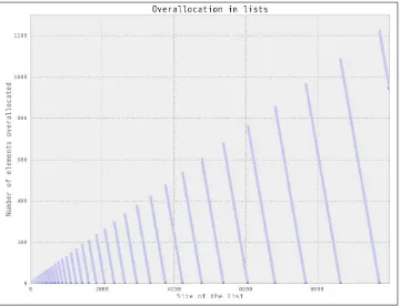
Problems with Allocating Too Much 106
Memory Fragmentation 109
Understanding perf 111
Making Decisions with perf ’s Output 113
Enter numpy 114
Applying numpy to the Diffusion Problem 117
Memory Allocations and In-Place Operations 120
Selective Optimizations: Finding What Needs to Be Fixed 124
numexpr: Making In-Place Operations Faster and Easier 127
A Cautionary Tale: Verify “Optimizations” (scipy) 129
Wrap-Up 130
7. Compiling to C. . . 135
What Sort of Speed Gains Are Possible? 136
JIT Versus AOT Compilers 138
Why Does Type Information Help the Code Run Faster? 138
Using a C Compiler 139
Reviewing the Julia Set Example 140
Cython 140
Bloom Filters 312
LogLog Counter 317
Real-World Example 321
12. Lessons from the Field. . . 325
Adaptive Lab’s Social Media Analytics (SoMA) 325
Python at Adaptive Lab 326
SoMA’s Design 326
Our Development Methodology 327
Maintaining SoMA 327
Advice for Fellow Engineers 328
Making Deep Learning Fly with RadimRehurek.com 328
The Sweet Spot 328
Lessons in Optimizing 330
Wrap-Up 332
Large-Scale Productionized Machine Learning at Lyst.com 333
Python’s Place at Lyst 333
Cluster Design 333
Code Evolution in a Fast-Moving Start-Up 333
Building the Recommendation Engine 334
Reporting and Monitoring 334
Some Advice 335
Large-Scale Social Media Analysis at Smesh 335
Python’s Role at Smesh 335
The Platform 336
High Performance Real-Time String Matching 336
Reporting, Monitoring, Debugging, and Deployment 338
PyPy for Successful Web and Data Processing Systems 339
Prerequisites 339
The Database 340
The Web Application 340
OCR and Translation 341
Task Distribution and Workers 341
Conclusion 341
Task Queues at Lanyrd.com 342
Python’s Role at Lanyrd 342
Making the Task Queue Performant 343
Reporting, Monitoring, Debugging, and Deployment 343
Advice to a Fellow Developer 343
Index. . . 345
Table of Contents | vii
Preface
Python is easy to learn. You’re probably here because now that your code runs correctly, you need it to run faster. You like the fact that your code is easy to modify and you can iterate with ideas quickly. The trade-off between easy to develop and runs as quickly as I need is a well-understood and often-bemoaned phenomenon. There are solutions. Some people have serial processes that have to run faster. Others have problems that could take advantage of multicore architectures, clusters, or graphics processing units. Some need scalable systems that can process more or less as expediency and funds allow, without losing reliability. Others will realize that their coding techniques, often bor‐ rowed from other languages, perhaps aren’t as natural as examples they see from others. In this book we will cover all of these topics, giving practical guidance for understanding bottlenecks and producing faster and more scalable solutions. We also include some war stories from those who went ahead of you, who took the knocks so you don’t have to.
Python is well suited for rapid development, production deployments, and scalable systems. The ecosystem is full of people who are working to make it scale on your behalf, leaving you more time to focus on the more challenging tasks around you.
Who This Book Is For
You’ve used Python for long enough to have an idea about why certain things are slow and to have seen technologies like Cython, numpy, and PyPy being discussed as possible solutions. You might also have programmed with other languages and so know that there’s more than one way to solve a performance problem.
While this book is primarily aimed at people with CPU-bound problems, we also look at data transfer and memory-bound solutions. Typically these problems are faced by scientists, engineers, quants, and academics.
We also look at problems that a web developer might face, including the movement of data and the use of just-in-time (JIT) compilers like PyPy for easy-win performance gains.
It might help if you have a background in C (or C++, or maybe Java), but it isn’t a pre-requisite. Python’s most common interpreter (CPython—the standard you normally get if you type python at the command line) is written in C, and so the hooks and libraries all expose the gory inner C machinery. There are lots of other techniques that we cover that don’t assume any knowledge of C.
You might also have a lower-level knowledge of the CPU, memory architecture, and data buses, but again, that’s not strictly necessary.
Who This Book Is Not For
This book is meant for intermediate to advanced Python programmers. Motivated nov‐ ice Python programmers may be able to follow along as well, but we recommend having a solid Python foundation.
We don’t cover storage-system optimization. If you have a SQL or NoSQL bottleneck, then this book probably won’t help you.
What You’ll Learn
Your authors have been working with large volumes of data, a requirement for I want the answers faster! and a need for scalable architectures, for many years in both industry and academia. We’ll try to impart our hard-won experience to save you from making the mistakes that we’ve made.
At the start of each chapter, we’ll list questions that the following text should answer (if it doesn’t, tell us and we’ll fix it in the next revision!).
We cover the following topics:
• Background on the machinery of a computer so you know what’s happening behind the scenes
• Lists and tuples—the subtle semantic and speed differences in these fundamental data structures
• Dictionaries and sets—memory allocation strategies and access algorithms in these important data structures
• Iterators—how to write in a more Pythonic way and open the door to infinite data streams using iteration
• Matrices with numpy—how to use the beloved numpy library like a beast
• Compilation and just-in-time computing—processing faster by compiling down to machine code, making sure you’re guided by the results of profiling
• Concurrency—ways to move data efficiently
• multiprocessing—the various ways to use the built-in multiprocessing library for parallel computing, efficiently share numpy matrices, and some costs and benefits of interprocess communication (IPC)
• Cluster computing—convert your multiprocessing code to run on a local or re‐ mote cluster for both research and production systems
• Using less RAM—approaches to solving large problems without buying a humun‐ gous computer
• Lessons from the field—lessons encoded in war stories from those who took the blows so you don’t have to
Python 2.7
Python 2.7 is the dominant version of Python for scientific and engineering computing. bit is dominant in this field, along with *nix environments (often Linux or Mac). 64-bit lets you address larger amounts of RAM. *nix lets you build applications that can be deployed and configured in well-understood ways with well-understood behaviors. If you’re a Windows user, then you’ll have to buckle up. Most of what we show will work just fine, but some things are OS-specific, and you’ll have to research a Windows solu‐ tion. The biggest difficulty a Windows user might face is the installation of modules: research in sites like StackOverflow should give you the solutions you need. If you’re on Windows, then having a virtual machine (e.g., using VirtualBox) with a running Linux installation might help you to experiment more freely.
Windows users should definitely look at a packaged solution like those available through Anaconda, Canopy, Python(x,y), or Sage. These same distributions will make the lives of Linux and Mac users far simpler too.
Moving to Python 3
Python 3 is the future of Python, and everyone is moving toward it. Python 2.7 will nonetheless be around for many years to come (some installations still use Python 2.4 from 2004); its retirement date has been set at 2020.
The shift to Python 3.3+ has caused enough headaches for library developers that people have been slow to port their code (with good reason), and therefore people have been slow to adopt Python 3. This is mainly due to the complexities of switching from a mix
of string and Unicode datatypes in complicated applications to the Unicode and byte implementation in Python 3.
Typically, when you want reproducible results based on a set of trusted libraries, you don’t want to be at the bleeding edge. High performance Python developers are likely to be using and trusting Python 2.7 for years to come.
Most of the code in this book will run with little alteration for Python 3.3+ (the most significant change will be with print turning from a statement into a function). In a few places we specifically look at improvements that Python 3.3+ provides. One item that might catch you out is the fact that / means integer division in Python 2.7, but it becomes float division in Python 3. Of course—being a good developer, your well-constructed unit test suite will already be testing your important code paths, so you’ll be alerted by your unit tests if this needs to be addressed in your code.
scipy and numpy have been Python 3–compatible since late 2010. matplotlib was compatible from 2012, scikit-learn was compatible in 2013, and NLTK is expected to be compatible in 2014. Django has been compatible since 2013. The transition notes for each are available in their repositories and newsgroups; it is worth reviewing the pro‐ cesses they used if you’re going to migrate older code to Python 3.
We encourage you to experiment with Python 3.3+ for new projects, but to be cautious with libraries that have only recently been ported and have few users—you’ll have a harder time tracking down bugs. It would be wise to make your code Python 3.3+-compatible (learn about the __future__ imports), so a future upgrade will be easier. Two good guides are “Porting Python 2 Code to Python 3” and “Porting to Python 3: An in-depth guide.” With a distribution like Anaconda or Canopy, you can run both Python 2 and Python 3 simultaneously—this will simplify your porting.
License
This book is licensed under Creative Commons Attribution-NonCommercial-NoDerivs 3.0.
You’re welcome to use this book for noncommercial purposes, including for noncommercial teaching. The license only allows for complete reproductions; for par‐ tial reproductions, please contact O’Reilly (see “How to Contact Us” on page xv). Please attribute the book as noted in the following section.
How to Make an Attribution
The Creative Commons license requires that you attribute your use of a part of this book. Attribution just means that you should write something that someone else can follow to find this book. The following would be sensible: “High Performance Python by Micha Gorelick and Ian Ozsvald (O’Reilly). Copyright 2014 Micha Gorelick and Ian Ozsvald, 978-1-449-36159-4.”
Errata and Feedback
We encourage you to review this book on public sites like Amazon—please help others understand if they’d benefit from this book! You can also email us at feedback@highper
formancepython.com.
We’re particularly keen to hear about errors in the book, successful use cases where the book has helped you, and high performance techniques that we should cover in the next edition. You can access the page for this book at http://bit.ly/High_Performance_Python. Complaints are welcomed through the instant-complaint-transmission-service > /dev/null.
Conventions Used in This Book
The following typographical conventions are used in this book: Italic
Indicates new terms, URLs, email addresses, filenames, and file extensions.
Constant width
Used for program listings, as well as within paragraphs to refer to commands, modules, and program elements such as variable or function names, databases, datatypes, environment variables, statements, and keywords.
Constant width bold
Shows commands or other text that should be typed literally by the user.
Constant width italic
Shows text that should be replaced with user-supplied values or by values deter‐ mined by context.
This element signifies a question or exercise.
This element signifies a general note.
This element indicates a warning or caution.
Using Code Examples
Supplemental material (code examples, exercises, etc.) is available for download at
https://github.com/mynameisfiber/high_performance_python.
This book is here to help you get your job done. In general, if example code is offered with this book, you may use it in your programs and documentation. You do not need to contact us for permission unless you’re reproducing a significant portion of the code. For example, writing a program that uses several chunks of code from this book does not require permission. Selling or distributing a CD-ROM of examples from O’Reilly books does require permission. Answering a question by citing this book and quoting example code does not require permission. Incorporating a significant amount of ex‐ ample code from this book into your product’s documentation does require permission. If you feel your use of code examples falls outside fair use or the permission given above, feel free to contact us at [email protected].
Safari® Books Online
Safari Books Online is an on-demand digital library that
delivers expert content in both book and video form from the world’s leading authors in technology and business.
Technology professionals, software developers, web designers, and business and creative professionals use Safari Books Online as their primary resource for research, problem solving, learning, and certification training.
Safari Books Online offers a range of plans and pricing for enterprise, government, education, and individuals.
Redbooks, Packt, Adobe Press, FT Press, Apress, Manning, New Riders, McGraw-Hill, Jones & Bartlett, Course Technology, and hundreds more. For more information about Safari Books Online, please visit us online.
How to Contact Us
Please address comments and questions concerning this book to the publisher:
O’Reilly Media, Inc.
1005 Gravenstein Highway North Sebastopol, CA 95472
800-998-9938 (in the United States or Canada) 707-829-0515 (international or local)
707-829-0104 (fax)
To comment or ask technical questions about this book, send email to bookques
For more information about our books, courses, conferences, and news, see our website
at http://www.oreilly.com.
Find us on Facebook: http://facebook.com/oreilly Follow us on Twitter: http://twitter.com/oreillymedia Watch us on YouTube: http://www.youtube.com/oreillymedia
Acknowledgments
Thanks to Jake Vanderplas, Brian Granger, Dan Foreman-Mackey, Kyran Dale, John Montgomery, Jamie Matthews, Calvin Giles, William Winter, Christian Schou Oxvig, Balthazar Rouberol, Matt “snakes” Reiferson, Patrick Cooper, and Michael Skirpan for invaluable feedback and contributions. Ian thanks his wife Emily for letting him dis‐ appear for 10 months to write this (thankfully she’s terribly understanding). Micha thanks Elaine and the rest of his friends and family for being so patient while he learned to write. O’Reilly are also rather lovely to work with.
Our contributors for the “Lessons from the Field” chapter very kindly shared their time and hard-won lessons. We give thanks to Ben Jackson, Radim Řehůřek, Sebastjan Treb‐ ca, Alex Kelly, Marko Tasic, and Andrew Godwin for their time and effort.
CHAPTER 1
Understanding Performant Python
Questions You’ll Be Able to Answer After This Chapter
• What are the elements of a computer’s architecture? • What are some common alternate computer architectures? • How does Python abstract the underlying computer architecture? • What are some of the hurdles to making performant Python code? • What are the different types of performance problems?
Programming computers can be thought of as moving bits of data and transforming them in special ways in order to achieve a particular result. However, these actions have a time cost. Consequently, high performance programming can be thought of as the act of minimizing these operations by either reducing the overhead (i.e., writing more ef‐ ficient code) or by changing the way that we do these operations in order to make each one more meaningful (i.e., finding a more suitable algorithm).
Let’s focus on reducing the overhead in code in order to gain more insight into the actual hardware on which we are moving these bits. This may seem like a futile exercise, since Python works quite hard to abstract away direct interactions with the hardware. How‐ ever, by understanding both the best way that bits can be moved in the real hardware and the ways that Python’s abstractions force your bits to move, you can make progress toward writing high performance programs in Python.
The Fundamental Computer System
The underlying components that make up a computer can be simplified into three basic parts: the computing units, the memory units, and the connections between them. In
addition, each of these units has different properties that we can use to understand them. The computational unit has the property of how many computations it can do per second, the memory unit has the properties of how much data it can hold and how fast we can read from and write to it, and finally the connections have the property of how fast they can move data from one place to another.
Using these building blocks, we can talk about a standard workstation at multiple levels of sophistication. For example, the standard workstation can be thought of as having a central processing unit (CPU) as the computational unit, connected to both the random access memory (RAM) and the hard drive as two separate memory units (each having different capacities and read/write speeds), and finally a bus that provides the connec‐ tions between all of these parts. However, we can also go into more detail and see that the CPU itself has several memory units in it: the L1, L2, and sometimes even the L3 and L4 cache, which have small capacities but very fast speeds (from several kilobytes to a dozen megabytes). These extra memory units are connected to the CPU with a special bus called the backside bus. Furthermore, new computer architectures generally come with new configurations (for example, Intel’s Nehalem CPUs replaced the front‐ side bus with the Intel QuickPath Interconnect and restructured many connections). Finally, in both of these approximations of a workstation we have neglected the network connection, which is effectively a very slow connection to potentially many other com‐ puting and memory units!
To help untangle these various intricacies, let’s go over a brief description of these fun‐ damental blocks.
Computing Units
The computing unit of a computer is the centerpiece of its usefulness—it provides the ability to transform any bits it receives into other bits or to change the state of the current process. CPUs are the most commonly used computing unit; however, graphics processing units (GPUs), which were originally typically used to speed up computer graphics but are becoming more applicable for numerical applications, are gaining popularity due to their intrinsically parallel nature, which allows many calculations to happen simultaneously. Regardless of its type, a computing unit takes in a series of bits (for example, bits representing numbers) and outputs another set of bits (for example, representing the sum of those numbers). In addition to the basic arithmetic operations on integers and real numbers and bitwise operations on binary numbers, some com‐ puting units also provide very specialized operations, such as the “fused multiply add” operation, which takes in three numbers, A,B,C, and returns the value A * B + C. The main properties of interest in a computing unit are the number of operations it can do in one cycle and how many cycles it can do in one second. The first value is measured
1. Not to be confused with interprocess communication, which shares the same acronym—we’ll look at the topic in Chapter 9.
by its instructions per cycle (IPC),1 while the latter value is measured by its clock speed.
These two measures are always competing with each other when new computing units are being made. For example, the Intel Core series has a very high IPC but a lower clock speed, while the Pentium 4 chip has the reverse. GPUs, on the other hand, have a very high IPC and clock speed, but they suffer from other problems, which we will outline later.
Furthermore, while increasing clock speed almost immediately speeds up all programs running on that computational unit (because they are able to do more calculations per second), having a higher IPC can also drastically affect computing by changing the level of vectorization that is possible. Vectorization is when a CPU is provided with multiple pieces of data at a time and is able to operate on all of them at once. This sort of CPU instruction is known as SIMD (Single Instruction, Multiple Data).
In general, computing units have been advancing quite slowly over the past decade (see Figure 1-1). Clock speeds and IPC have both been stagnant because of the physical limitations of making transistors smaller and smaller. As a result, chip manufacturers have been relying on other methods to gain more speed, including hyperthreading, more clever out-of-order execution, and multicore architectures.
Hyperthreading presents a virtual second CPU to the host operating system (OS), and clever hardware logic tries to interleave two threads of instructions into the execution units on a single CPU. When successful, gains of up to 30% over a single thread can be achieved. Typically this works well when the units of work across both threads use different types of execution unit—for example, one performs floating-point operations and the other performs integer operations.
Out-of-order execution enables a compiler to spot that some parts of a linear program sequence do not depend on the results of a previous piece of work, and therefore that both pieces of work could potentially occur in any order or at the same time. As long as sequential results are presented at the right time, the program continues to execute correctly, even though pieces of work are computed out of their programmed order. This enables some instructions to execute when others might be blocked (e.g., waiting for a memory access), allowing greater overall utilization of the available resources. Finally, and most important for the higher-level programmer, is the prevalence of multi-core architectures. These architectures include multiple CPUs within the same unit, which increases the total capability without running into barriers in making each in‐ dividual unit faster. This is why it is currently hard to find any machine with less than two cores—in this case, the computer has two physical computing units that are con‐ nected to each other. While this increases the total number of operations that can be
done per second, it introduces intricacies in fully utilizing both computing units at the same time.
Figure 1-1. Clock speed of CPUs over time (data from CPU DB)
Simply adding more cores to a CPU does not always speed up a program’s execution time. This is because of something known as Amdahl’s law. Simply stated, Amdahl’s law says that if a program designed to run on multiple cores has some routines that must run on one core, this will be the bottleneck for the final speedup that can be achieved by allocating more cores.
For example, if we had a survey we wanted 100 people to fill out, and that survey took 1 minute to complete, we could complete this task in 100 minutes if we had one person asking the questions (i.e., this person goes to participant 1, asks the questions, waits for the responses, then moves to participant 2). This method of having one person asking the questions and waiting for responses is similar to a serial process. In serial processes, we have operations being satisfied one at a time, each one waiting for the previous operation to complete.
each individual person asking the questions does not need to know anything about the other person asking questions. As a result, the task can be easily split up without having any dependency between the question askers.
Adding more people asking the questions will give us more speedups, until we have 100 people asking questions. At this point, the process would take 1 minute and is simply limited by the time it takes the participant to answer questions. Adding more people asking questions will not result in any further speedups, because these extra people will have no tasks to perform—all the participants are already being asked questions! At this point, the only way to reduce the overall time to run the survey is to reduce the amount of time it takes for an individual survey, the serial portion of the problem, to complete. Similarly, with CPUs, we can add more cores that can perform various chunks of the computation as necessary until we reach a point where the bottleneck is a specific core finishing its task. In other words, the bottleneck in any parallel calculation is always the smaller serial tasks that are being spread out.
Furthermore, a major hurdle with utilizing multiple cores in Python is Python’s use of a global interpreter lock (GIL). The GIL makes sure that a Python process can only run one instruction at a time, regardless of the number of cores it is currently using. This means that even though some Python code has access to multiple cores at a time, only one core is running a Python instruction at any given time. Using the previous example of a survey, this would mean that even if we had 100 question askers, only one could ask a question and listen to a response at a time. This effectively removes any sort of benefit from having multiple question askers! While this may seem like quite a hurdle, especially if the current trend in computing is to have multiple computing units rather than having faster ones, this problem can be avoided by using other standard library tools, like multiprocessing, or technologies such as numexpr, Cython, or distributed models of computing.
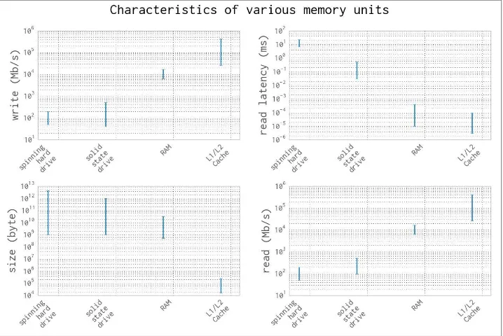
Memory Units
Memory units in computers are used to store bits. This could be bits representing vari‐ ables in your program, or bits representing the pixels of an image. Thus, the abstraction of a memory unit applies to the registers in your motherboard as well as your RAM and hard drive. The one major difference between all of these types of memory units is the speed at which they can read/write data. To make things more complicated, the read/ write speed is heavily dependent on the way that data is being read.
For example, most memory units perform much better when they read one large chunk of data as opposed to many small chunks (this is referred to as sequential read versus random data). If the data in these memory units is thought of like pages in a large book, this means that most memory units have better read/write speeds when going through the book page by page rather than constantly flipping from one random page to another.
While this fact is generally true across all memory units, the amount that this affects each type is drastically different.
In addition to the read/write speeds, memory units also have latency, which can be characterized as the time it takes the device to find the data that is being used. For a spinning hard drive, this latency can be high because the disk needs to physically spin up to speed and the read head must move to the right position. On the other hand, for RAM this can be quite small because everything is solid state. Here is a short description of the various memory units that are commonly found inside a standard workstation, in order of read/write speeds:
Spinning hard drive
Long-term storage that persists even when the computer is shut down. Generally has slow read/write speeds because the disk must be physically spun and moved. Degraded performance with random access patterns but very large capacity (tera‐ byte range).
Solid state hard drive
Similar to a spinning hard drive, with faster read/write speeds but smaller capacity (gigabyte range).
RAM
Used to store application code and data (such as any variables being used). Has fast read/write characteristics and performs well with random access patterns, but is generally limited in capacity (gigabyte range).
L1/L2 cache
Extremely fast read/write write speeds. Data going to the CPU must go through here. Very small capacity (kilobyte range).
Figure 1-2 gives a graphic representation of the differences between these types of memory units by looking at the characteristics of currently available consumer hardware.
Figure 1-2. Characteristic values for different types of memory units (values from Feb‐ ruary 2014)
Communications Layers
Finally, let’s look at how all of these fundamental blocks communicate with each other. There are many different modes of communication, but they are all variants on a thing called a bus.
The frontside bus, for example, is the connection between the RAM and the L1/L2 cache. It moves data that is ready to be transformed by the processor into the staging ground to get ready for calculation, and moves finished calculations out. There are other buses, too, such as the external bus that acts as the main route from hardware devices (such as hard drives and networking cards) to the CPU and system memory. This bus is generally slower than the frontside bus.
In fact, many of the benefits of the L1/L2 cache are attributable to the faster bus. Being able to queue up data necessary for computation in large chunks on a slow bus (from RAM to cache) and then having it available at very fast speeds from the backside bus (from cache to CPU) enables the CPU to do more calculations without waiting such a long time.
Similarly, many of the drawbacks of using a GPU come from the bus it is connected on: since the GPU is generally a peripheral device, it communicates through the PCI bus,
which is much slower than the frontside bus. As a result, getting data into and out of the GPU can be quite a taxing operation. The advent of heterogeneous computing, or computing blocks that have both a CPU and a GPU on the frontside bus, aims at reducing the data transfer cost and making GPU computing more of an available option, even when a lot of data must be transferred.
In addition to the communication blocks within the computer, the network can be thought of as yet another communication block. This block, however, is much more pliable than the ones discussed previously; a network device can be connected to a memory device, such as a network attached storage (NAS) device or another computing block, as in a computing node in a cluster. However, network communications are gen‐ erally much slower than the other types of communications mentioned previously. While the frontside bus can transfer dozens of gigabits per second, the network is limited to the order of several dozen megabits.
It is clear, then, that the main property of a bus is its speed: how much data it can move in a given amount of time. This property is given by combining two quantities: how much data can be moved in one transfer (bus width) and how many transfers it can do per second (bus frequency). It is important to note that the data moved in one transfer is always sequential: a chunk of data is read off of the memory and moved to a different place. Thus, the speed of a bus is broken up into these two quantities because individually they can affect different aspects of computation: a large bus width can help vectorized code (or any code that sequentially reads through memory) by making it possible to move all the relevant data in one transfer, while, on the other hand, having a small bus width but a very high frequency of transfers can help code that must do many reads from random parts of memory. Interestingly, one of the ways that these properties are changed by computer designers is by the physical layout of the motherboard: when chips are placed closed to one another, the length of the physical wires joining them is smaller, which can allow for faster transfer speeds. In addition, the number of wires itself dictates the width of the bus (giving real physical meaning to the term!).
Figure 1-3. Connection speeds of various common interfaces (image by Leadbuffalo [CC BY-SA 3.0])
Putting the Fundamental Elements Together
Understanding the basic components of a computer is not enough to fully understand the problems of high performance programming. The interplay of all of these components and how they work together to solve a problem introduces extra levels of complexity. In this section we will explore some toy problems, illustrating how the ideal solutions would work and how Python approaches them.
A warning: this section may seem bleak—most of the remarks seem to say that Python is natively incapable of dealing with the problems of performance. This is untrue, for two reasons. Firstly, in all of these “components of performant computing” we have
neglected one very important component: the developer. What native Python may lack in performance it gets back right away with speed of development. Furthermore, throughout the book we will introduce modules and philosophies that can help mitigate many of the problems described here with relative ease. With both of these aspects combined, we will keep the fast development mindset of Python while removing many of the performance constraints.
Idealized Computing Versus the Python Virtual Machine
In order to better understand the components of high performance programming, let us look at a simple code sample that checks if a number is prime:
import math
def check_prime(number):
sqrt_number = math.sqrt(number)
number_float = float(number)
for i in xrange(2, int(sqrt_number)+1):
if (number_float / i).is_integer():
return False
return True
print "check_prime(10000000) = ", check_prime(10000000) # False print "check_prime(10000019) = ", check_prime(10000019) # True
Let’s analyze this code using our abstract model of computation and then draw com‐ parisons to what happens when Python runs this code. As with any abstraction, we will neglect many of the subtleties in both the idealized computer and the way that Python runs the code. However, this is generally a good exercise to perform before solving a problem: think about the general components of the algorithm and what would be the best way for the computing components to come together in order to find a solution. By understanding this ideal situation and having knowledge of what is actually hap‐ pening under the hood in Python, we can iteratively bring our Python code closer to the optimal code.
Idealized computing
optimization. The concept of “heavy data” refers to the fact that it takes time and effort to move data around, which is something we would like to avoid.
For the loop in the code, rather than sending one value of i at a time to the CPU, we would like to send it both number_float and several values of i to check at the same time. This is possible because the CPU vectorizes operations with no additional time cost, meaning it can do multiple independent computations at the same time. So, we want to send number_float to the CPU cache, in addition to as many values of i as the cache can hold. For each of the number_float/i pairs, we will divide them and check if the result is a whole number; then we will send a signal back indicating whether any of the values was indeed an integer. If so, the function ends. If not, we repeat. In this way, we only need to communicate back one result for many values of i, rather than de‐ pending on the slow bus for every value. This takes advantage of a CPU’s ability to vectorize a calculation, or run one instruction on multiple data in one clock cycle. This concept of vectorization is illustrated by the following code:
import math
def check_prime(number):
sqrt_number = math.sqrt(number)
number_float = float(number)
numbers = range(2, int(sqrt_number)+1)
for i in xrange(0, len(numbers), 5):
# the following line is not valid Python code
result = (number_float / numbers[i:(i+5)]).is_integer()
if any(result):
return False
return True
Here, we set up the processing such that the division and the checking for integers are done on a set of five values of i at a time. If properly vectorized, the CPU can do this line in one step as opposed to doing a separate calculation for every i. Ideally, the any(result) operation would also happen in the CPU without having to transfer the results back to RAM. We will talk more about vectorization, how it works, and when it benefits your code in Chapter 6.
Python’s virtual machine
The Python interpreter does a lot of work to try to abstract away the underlying com‐ puting elements that are being used. At no point does a programmer need to worry about allocating memory for arrays, how to arrange that memory, or in what sequence it is being sent to the CPU. This is a benefit of Python, since it lets you focus on the algorithms that are being implemented. However, it comes at a huge performance cost. It is important to realize that at its core, Python is indeed running a set of very optimized instructions. The trick, however, is getting Python to perform them in the correct se‐ quence in order to achieve better performance. For example, it is quite easy to see that,
in the following example, search_fast will run faster than search_slow simply because it skips the unnecessary computations that result from not terminating the loop early, even though both solutions have runtime O(n).
def search_fast(haystack, needle):
Identifying slow regions of code through profiling and finding more efficient ways of doing the same calculations is similar to finding these useless operations and removing them; the end result is the same, but the number of computations and data transfers is reduced drastically.
One of the impacts of this abstraction layer is that vectorization is not immediately achievable. Our initial prime number routine will run one iteration of the loop per value of i instead of combining several iterations. However, looking at the abstracted vecto‐ rization example, we see that it is not valid Python code, since we cannot divide a float by a list. External libraries such as numpy will help with this situation by adding the ability to do vectorized mathematical operations.
Furthermore, Python’s abstraction hurts any optimizations that rely on keeping the L1/ L2 cache filled with the relevant data for the next computation. This comes from many factors, the first being that Python objects are not laid out in the most optimal way in memory. This is a consequence of Python being a garbage-collected language—memory is automatically allocated and freed when needed. This creates memory fragmentation that can hurt the transfers to the CPU caches. In addition, at no point is there an op‐ portunity to change the layout of a data structure directly in memory, which means that one transfer on the bus may not contain all the relevant information for a computation, even though it might have all fit within the bus width.
A second, more fundamental problem comes from Python’s dynamic types and it not being compiled. As many C programmers have learned throughout the years, the com‐ piler is often smarter than you are. When compiling code that is static, the compiler can do many tricks to change the way things are laid out and how the CPU will run certain instructions in order to optimize them. Python, however, is not compiled: to make matters worse, it has dynamic types, which means that inferring any possible opportu‐ nities for optimizations algorithmically is drastically harder since code functionality can be changed during runtime. There are many ways to mitigate this problem, foremost
being use of Cython, which allows Python code to be compiled and allows the user to create “hints” to the compiler as to how dynamic the code actually is.
Finally, the previously mentioned GIL can hurt performance if trying to parallelize this code. For example, let’s assume we change the code to use multiple CPU cores such that each core gets a chunk of the numbers from 2 to sqrtN. Each core can do its calculation for its chunk of numbers and then, when they are all done, they can compare their calculations. This seems like a good solution since, although we lose the early termina‐ tion of the loop, we can reduce the number of checks each core has to do by the number of cores we are using (i.e., if we had M cores, each core would have to do sqrtN / M checks). However, because of the GIL, only one core can be used at a time. This means that we would effectively be running the same code as the unparallelled version, but we no longer have early termination. We can avoid this problem by using multiple processes (with the multiprocessing module) instead of multiple threads, or by using Cython or foreign functions.
So Why Use Python?
Python is highly expressive and easy to learn—new programmers quickly discover that they can do quite a lot in a short space of time. Many Python libraries wrap tools written in other languages to make it easy to call other systems; for example, the scikit-learn machine learning system wraps LIBLINEAR and LIBSVM (both of which are written in C), and the numpy library includes BLAS and other C and Fortran libraries. As a result, Python code that properly utilizes these modules can indeed be as fast as comparable C code.
Python is described as “batteries included,” as many important and stable libraries are built in. These include:
unicode and bytes
Baked into the core language
array
Memory-efficient arrays for primitive types
math
Basic mathematical operations, including some simple statistics
sqlite3
A wrapper around the prevalent SQL file-based storage engine SQLite3
collections
A wide variety of objects, including a deque, counter, and dictionary variants Outside of the core language there is a huge variety of libraries, including:
numpy
a numerical Python library (a bedrock library for anything to do with matrices)
scipy
a very large collection of trusted scientific libraries, often wrapping highly respected C and Fortran libraries
pandas
a library for data analysis, similar to R’s data frames or an Excel spreadsheet, built on scipy and numpy
scikit-learn
rapidly turning into the default machine learning library, built on scipy
biopython
a bioinformatics library similar to bioperl
tornado
a library that provides easy bindings for concurrency
Database bindings
for communicating with virtually all databases, including Redis, MongoDB, HDF5, and SQL
Web development frameworks
performant systems for creating websites such as django, pyramid, flask, and tornado
OpenCV
bindings for computer vision
API bindings
for easy access to popular web APIs such as Google, Twitter, and LinkedIn A large selection of managed environments and shells is available to fit various deploy‐ ment scenarios, including:
• The standard distribution, available at http://python.org
• Enthought’s EPD and Canopy, a very mature and capable environment • Continuum’s Anaconda, a scientifically focused environment
• Sage, a Matlab-like environment including an integrated development environment (IDE)
• Python(x,y)
• IPython Notebook, a browser-based frontend to IPython, heavily used for teaching and demonstrations
• BPython, interactive Python shell
One of Python’s main strengths is that it enables fast prototyping of an idea. Due to the wide variety of supporting libraries it is easy to test if an idea is feasible, even if the first implementation might be rather flaky.
If you want to make your mathematical routines faster, look to numpy. If you want to experiment with machine learning, try scikit-learn. If you are cleaning and manip‐ ulating data, then pandas is a good choice.
In general, it is sensible to raise the question, “If our system runs faster, will we as a team run slower in the long run?” It is always possible to squeeze more performance out of a system if enough man-hours are invested, but this might lead to brittle and poorly understood optimizations that ultimately trip the team up.
One example might be the introduction of Cython (“Cython” on page 140), a compiler-based approach to annotating Python code with C-like types so the transformed code can be compiled using a C compiler. While the speed gains can be impressive (often achieving C-like speeds with relatively little effort), the cost of supporting this code will increase. In particular, it might be harder to support this new module, as team members will need a certain maturity in their programming ability to understand some of the trade-offs that have occurred when leaving the Python virtual machine that introduced the performance increase.
CHAPTER 2
Profiling to Find Bottlenecks
Questions You’ll Be Able to Answer After This Chapter
• How can I identify speed and RAM bottlenecks in my code? • How do I profile CPU and memory usage?
• What depth of profiling should I use?
• How can I profile a long-running application? • What’s happening under the hood with CPython?
• How do I keep my code correct while tuning performance?
Profiling lets us find bottlenecks so we can do the least amount of work to get the biggest practical performance gain. While we’d like to get huge gains in speed and reductions in resource usage with little work, practically you’ll aim for your code to run “fast enough” and “lean enough” to fit your needs. Profiling will let you make the most prag‐ matic decisions for the least overall effort.
Any measurable resource can be profiled (not just the CPU!). In this chapter we look at both CPU time and memory usage. You could apply similar techniques to measure network bandwidth and disk I/O too.
If a program is running too slowly or using too much RAM, then you’ll want to fix whichever parts of your code are responsible. You could, of course, skip profiling and fix what you believe might be the problem—but be wary, as you’ll often end up “fixing” the wrong thing. Rather than using your intuition, it is far more sensible to first profile, having defined a hypothesis, before making changes to the structure of your code.
Sometimes it’s good to be lazy. By profiling first, you can quickly identify the bottlenecks that need to be solved, and then you can solve just enough of these to achieve the performance you need. If you avoid profiling and jump to optimization, then it is quite likely that you’ll do more work in the long run. Always be driven by the results of profiling.
Profiling Efficiently
The first aim of profiling is to test a representative system to identify what’s slow (or using too much RAM, or causing too much disk I/O or network I/O). Profiling typically adds an overhead (10x to 100x slowdowns can be typical), and you still want your code to be used as similarly to in a real-world situation as possible. Extract a test case and isolate the piece of the system that you need to test. Preferably, it’ll have been written to be in its own set of modules already.
The basic techniques that are introduced first in this chapter include the %timeit magic in IPython, time.time(), and a timing decorator. You can use these techniques to un‐ derstand the behavior of statements and functions.
Then we will cover cProfile (“Using the cProfile Module” on page 31), showing you how to use this built-in tool to understand which functions in your code take the longest to run. This will give you a high-level view of the problem so you can direct your at‐ tention to the critical functions.
Next, we’ll look at line_profiler (“Using line_profiler for Line-by-Line Measure‐ ments” on page 37), which will profile your chosen functions on a line-by-line basis. The result will include a count of the number of times each line is called and the percentage of time spent on each line. This is exactly the information you need to understand what’s running slowly and why.
Armed with the results of line_profiler, you’ll have the information you need to move on to using a compiler (Chapter 7).
In Chapter 6 (Example 6-8), you’ll learn how to use perf stat to understand the number of instructions that are ultimately executed on a CPU and how efficiently the CPU’s caches are utilized. This allows for advanced-level tuning of matrix operations. You should take a look at that example when you’re done with this chapter.
To help you understand why your RAM usage is high, we’ll show you memory_profil er (“Using memory_profiler to Diagnose Memory Usage” on page 42). It is particularly useful for tracking RAM usage over time on a labeled chart, so you can explain to colleagues why certain functions use more RAM than expected.
Whatever approach you take to profiling your code, you must re‐ member to have adequate unit test coverage in your code. Unit tests help you to avoid silly mistakes and help to keep your results repro‐ ducible. Avoid them at your peril.
Always profile your code before compiling or rewriting your algo‐ rithms. You need evidence to determine the most efficient ways to make your code run faster.
Finally, we’ll give you an introduction to the Python bytecode inside CPython (“Using the dis Module to Examine CPython Bytecode” on page 52), so you can understand what’s happening “under the hood.” In particular, having an understanding of how Python’s stack-based virtual machine operates will help you to understand why certain coding styles run more slowly than others.
Before the end of the chapter, we’ll review how to integrate unit tests while profiling (“Unit Testing During Optimization to Maintain Correctness” on page 56), to preserve the correctness of your code while you make it run more efficiently.
We’ll finish with a discussion of profiling strategies (“Strategies to Profile Your Code Successfully” on page 59), so you can reliably profile your code and gather the correct data to test your hypotheses. Here you’ll learn about how dynamic CPU frequency scaling and features like TurboBoost can skew your profiling results and how they can be disabled.
To walk through all of these steps, we need an easy-to-analyze function. The next section introduces the Julia set. It is a CPU-bound function that’s a little hungry for RAM; it also exhibits nonlinear behavior (so we can’t easily predict the outcomes), which means we need to profile it at runtime rather than analyzing it offline.
Introducing the Julia Set
The Julia set is an interesting CPU-bound problem for us to begin with. It is a fractal sequence that generates a complex output image, named after Gaston Julia.
The code that follows is a little longer than a version you might write yourself. It has a CPU-bound component and a very explicit set of inputs. This configuration allows us to profile both the CPU usage and the RAM usage so we can understand which parts of our code are consuming two of our scarce computing resources. This implementation is deliberately suboptimal, so we can identify memory-consuming operations and slow
statements. Later in this chapter we’ll fix a slow logic statement and a memory-consuming statement, and in Chapter 7 we’ll significantly speed up the overall execution time of this function.
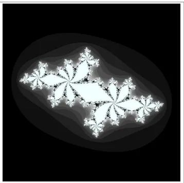
We will analyze a block of code that produces both a false grayscale plot (Figure 2-1) and a pure grayscale variant of the Julia set (Figure 2-3), at the complex point c=-0.62772-0.42193j. A Julia set is produced by calculating each pixel in isolation; this is an “embarrassingly parallel problem” as no data is shared between points.
Figure 2-1. Julia set plot with a false grayscale to highlight detail
The problem is interesting because we calculate each pixel by applying a loop that could be applied an indeterminate number of times. On each iteration we test to see if this coordinate’s value escapes toward infinity, or if it seems to be held by an attractor. Coordinates that cause few iterations are colored darkly in Figure 2-1, and those that cause a high number of iterations are colored white. White regions are more complex to calculate and so take longer to generate.
We define a set of z-coordinates that we’ll test. The function that we calculate squares the complex number z and adds c:
f(z) =z2+c
We iterate on this function while testing to see if the escape condition holds using abs. If the escape function is False, then we break out of the loop and record the number of iterations we performed at this coordinate. If the escape function is never False, then we stop after maxiter iterations. We will later turn this z’s result into a colored pixel representing this complex location.
In pseudocode, it might look like:
for z in coordinates:
for iteration in range(maxiter): # limited iterations per point if abs(z) < 2.0: # has the escape condition been broken? z = z*z + c
else:
break
# store the iteration count for each z and draw later
To explain this function, let’s try two coordinates.
First, we’ll use the coordinate that we draw in the top-left corner of the plot at -1.8-1.8j. We must test abs(z) < 2 before we can try the update rule:
z = -1.8-1.8j print abs(z)
2.54558441227
We can see that for the top-left coordinate the abs(z) test will be False on the zeroth iteration, so we do not perform the update rule. The output value for this coordinate is 0.
Now let’s jump to the center of the plot at z = 0 + 0j and try a few iterations:
c = -0.62772-0.42193j
z = 0+0j
for n in range(9):
z = z*z + c
print "{}: z={:33}, abs(z)={:0.2f}, c={}".format(n, z, abs(z), c)
0: z= (-0.62772-0.42193j), abs(z)=0.76, c=(-0.62772-0.42193j) 1: z= (-0.4117125265+0.1077777992j), abs(z)=0.43, c=(-0.62772-0.42193j) 2: z=(-0.469828849523-0.510676940018j), abs(z)=0.69, c=(-0.62772-0.42193j) 3: z=(-0.667771789222+0.057931518414j), abs(z)=0.67, c=(-0.62772-0.42193j) 4: z=(-0.185156898345-0.499300067407j), abs(z)=0.53, c=(-0.62772-0.42193j) 5: z=(-0.842737480308-0.237032296351j), abs(z)=0.88, c=(-0.62772-0.42193j) 6: z=(0.026302151203-0.0224179996428j), abs(z)=0.03, c=(-0.62772-0.42193j) 7: z= (-0.62753076355-0.423109283233j), abs(z)=0.76, c=(-0.62772-0.42193j) 8: z=(-0.412946606356+0.109098183144j), abs(z)=0.43, c=(-0.62772-0.42193j)
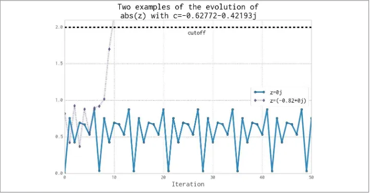
We can see that each update to z for these first iterations leaves it with a value where abs(z) < 2 is True. For this coordinate we can iterate 300 times, and still the test will be True. We cannot tell how many iterations we must perform before the condition becomes False, and this may be an infinite sequence. The maximum iteration (maxit er) break clause will stop us iterating potentially forever.
In Figure 2-2 we see the first 50 iterations of the preceding sequence. For 0+0j (the solid line with circle markers) the sequence appears to repeat every eighth iteration, but each sequence of seven calculations has a minor deviation from the previous sequence—we can’t tell if this point will iterate forever within the boundary condition, or for a long time, or maybe for just a few more iterations. The dashed cutoff line shows the bound‐ ary at +2.
Figure 2-2. Two coordinate examples evolving for the Julia set
For -0.82+0j (the dashed line with diamond markers), we can see that after the ninth update the absolute result has exceeded the +2 cutoff, so we stop updating this value.
Calculating the Full Julia Set
In this section we break down the code that generates the Julia set. We’ll analyze it in various ways throughout this chapter. As shown in Example 2-1, at the start of our module we import the time module for our first profiling approach and define some coordinate constants.
Example 2-1. Defining global constants for the coordinate space """Julia set generator without optional PIL-based image drawing""" import time
# area of complex space to investigate
x1, x2, y1, y2 = -1.8, 1.8, -1.8, 1.8
c_real, c_imag = -0.62772, -.42193
To generate the plot, we create two lists of input data. The first is zs (complex z -coordinates), and the second is cs (a complex initial condition). Neither list varies, and we could optimize cs to a single c value as a constant. The rationale for building two input lists is so that we have some reasonable-looking data to profile when we profile RAM usage later in this chapter.
To build the zs and cs lists, we need to know the coordinates for each z. In Example 2-2 we build up these coordinates using xcoord and ycoord and a specified x_step and y_step. The somewhat verbose nature of this setup is useful when porting the code to other tools (e.g., to numpy) and to other Python environments, as it helps to have ev‐ erything very clearly defined for debugging.
Example 2-2. Establishing the coordinate lists as inputs to our calculation function def calc_pure_python(desired_width, max_iterations):
"""Create a list of complex coordinates (zs) and complex parameters (cs), build Julia set, and display""" x_step = (float(x2 - x1) / float(desired_width))
# Build a list of coordinates and the initial condition for each cell. # Note that our initial condition is a constant and could easily be removed; # we use it to simulate a real-world scenario with several inputs to
# our function. zs = []
cs = []
for ycoord in y:
for xcoord in x:
zs.append(complex(xcoord, ycoord))
cs.append(complex(c_real, c_imag))
print "Length of x:", len(x)
print "Total elements:", len(zs)
start_time = time.time()
output = calculate_z_serial_purepython(max_iterations, zs, cs)
end_time = time.time()
secs= end_time - start_time
print calculate_z_serial_purepython.func_name + " took", secs, "seconds"
# This sum is expected for a 1000^2 grid with 300 iterations. # It catches minor errors we might introduce when we're # working on a fixed set of inputs.
assert sum(output) == 33219980
Having built the zs and cs lists, we output some information about the size of the lists and calculate the output list via calculate_z_serial_purepython. Finally, we sum the contents of output and assert that it matches the expected output value. Ian uses it here to confirm that no errors creep into the book.
As the code is deterministic, we can verify that the function works as we expect by summing all the calculated values. This is useful as a sanity check—when we make changes to numerical code it is very sensible to check that we haven’t broken the algo‐ rithm. Ideally we would use unit tests and we’d test more than one configuration of the problem.
Example 2-3. Our CPU-bound calculation function def calculate_z_serial_purepython(maxiter, zs, cs):
"""Calculate output list using Julia update rule""" output = [0] * len(zs)
for i in range(len(zs)):
n = 0 z = zs[i]
c = cs[i]
while abs(z) < 2 and n < maxiter:
z = z * z + c
n += 1 output[i] = n
return output
Now we call the calculation routine in Example 2-4. By wrapping it in a __main__ check, we can safely import the module without starting the calculations for some of the profiling methods. Note that here we’re not showing the method used to plot the output.
Example 2-4. main for our code if __name__ == "__main__":
# Calculate the Julia set using a pure Python solution with # reasonable defaults for a laptop
calc_pure_python(desired_width=1000, max_iterations=300)
Once we run the code, we see some output about the complexity of the problem:
# running the above produces:
Length of x: 1000
Total elements: 1000000
calculate_z_serial_purepython took 12.3479790688 seconds
In the false-grayscale plot (Figure 2-1), the high-contrast color changes gave us an idea of where the cost of the function was slow-changing or fast-changing. Here, in Figure 2-3, we have a linear color map: black is quick to calculate and white is expensive to calculate.
By showing two representations of the same data, we can see that lots of detail is lost in the linear mapping. Sometimes it can be useful to have various representations in mind when investigating the cost of a function.
Figure 2-3. Julia plot example using a pure grayscale
Simple Approaches to Timing—print and a Decorator
After Example 2-4, we saw the output generated by several print statements in our code. On Ian’s laptop this code takes approximately 12 seconds to run using CPython 2.7. It is useful to note that there is always some variation in execution time. You must observe the normal variation when you’re timing your code, or you might incorrectly attribute an improvement in your code simply to a random variation in execution time. Your computer will be performing other tasks while running your code, such as accessing the network, disk, or RAM, and these factors can cause variations in the ex‐ ecution time of your program.Ian’s laptop is a Dell E6420 with an Intel Core I7-2720QM CPU (2.20 GHz, 6 MB cache, Quad Core) and 8 GB of RAM running Ubuntu 13.10.
In calc_pure_python (Example 2-2), we can see several print statements. This is the simplest way to measure the execution time of a piece of code inside a function. It is a very basic approach, but despite being quick and dirty it can be very useful when you’re first looking at a piece of code.
A slightly cleaner approach is to use a decorator—here, we add one line of code above the function that we care about. Our decorator can be very simple and just replicate the effect of the print statements. Later, we can make it more advanced.
In Example 2-5 we define a new function, timefn, which takes a function as an argument: the inner function, measure_time, takes *args (a variable number of positional argu‐ ments) and **kwargs (a variable number of key/value arguments) and passes them through to fn for execution. Around the execution of fn we capture time.time() and then print the result along with fn.func_name. The overhead of using this decorator is small, but if you’re calling fn millions of times the overhead might become noticeable. We use @wraps(fn) to expose the function name and docstring to the caller of the decorated function (otherwise, we would see the function name and docstring for the decorator, not the function it decorates).
Example 2-5. Defining a decorator to automate timing measurements from functools import wraps
def timefn(fn):
@wraps(fn)
def measure_time(*args, **kwargs):
t1 = time.time()
result = fn(*args, **kwargs)
t2 = time.time()
print ("@timefn:" + fn.func_name + " took " + str(t2 - t1) + " seconds")
return result
return measure_time
@timefn
def calculate_z_serial_purepython(maxiter, zs, cs):
...
When we run this version (we keep the print statements from before), we can see that the execution time in the decorated version is very slightly quicker than the call from calc_pure_python. This is due to the overhead of calling a function (the difference is very tiny):
Length of x: 1000
Total elements: 1000000
@timefn:calculate_z_serial_purepython took 12.2218790054 seconds calculate_z_serial_purepython took 12.2219250043 seconds
The addition of profiling information will inevitably slow your code down—some profiling options are very informative and induce a heavy speed penalty. The trade-off between profiling detail and speed will be something you have to consider.

![Figure 1-3. Connection speeds of various common interfaces (image by Leadbuffalo[CC BY-SA 3.0])](https://thumb-ap.123doks.com/thumbv2/123dok/3935161.1878581/27.504.72.435.51.411/figure-connection-speeds-various-common-interfaces-image-leadbuffalo.webp)