*Corresponding author. Tel.:#1-405-325-3444/1-405-325-5591; fax:#1-405-325-1957.
E-mail address:[email protected] (S.C. Linn).
Fuzzy inductive reasoning, expectation
formation and the behavior of
security prices
Nicholas S.P. Tay
!
, Scott C. Linn
",
*
!McLaren School of Business, University of San Francisco, San Francisco, CA 94117, USA "Division of Finance, Michael F. Price College of Business, 205 A Adams Hall,
University of Oklahoma, Norman, OK 73019, USA
Accepted 22 February 2000
Abstract
This paper extends the Santa Fe Arti"cial Stock Market Model (SFASM) studied by LeBaron, Arthur and Palmer (1999, Journal of Economic Dynamics and Control 23, 1487}1516) in two important directions. First, some might question whether it is reason-able to assume that traders are capreason-able of handling a large number of rules, each with numerous conditions, as is assumed in the SFASM. We demonstrate that similar results can be obtained even after severely limiting the reasoning process. We show this by allowing agents the ability to compress information into a few fuzzy notions which they can in turn process and analyze with fuzzy logic. Second, LeBaron et al. have reported that the kurtosis of their simulated stock returns is too small as compared to real data. We demonstrate that with a minor modi"cation to how traders go about deciding which of their prediction rules to rely on when making demand decisions, the model can in fact produce return kurtosis that is comparable to that of actual returns data. ( 2001 Elsevier Science B.V. All rights reserved.
JEL classixcation: G12; G14; D83; D84
Keywords: Expectations; Learning; Fuzzy logic; Induction; Stock price dynamics
1LeBaron (2000) presents a comprehensive review of the emerging literature that has come to be known as&agent-based computational economics/"nance'. The present paper contributes to this literature. See also Brock and Hommes (1998).
1. Introduction
Neoclassical"nancial market models are generally formulated so economic
agents are able to logically deduce their price expectations. Real stock markets do not however typically conform to the severe restrictions required to guaran-tee such behavior. In fact, the actual market environment is usually much more ill-de"ned. The dilemma is that in an ill-de"ned environment the ability to exercise deductive reasoning breaks down, making it impossible for individuals to form precise and objective price expectations. This implies that participants
in real "nancial markets must rely on some alternative form of reasoning to
guide their decision making. We conjecture that individual reasoning in an ill-de"ned setting can be described as an inductive process in which individuals exhibit limitations in their abilities to process and condense information. The reasoning process we postulate is melded with a model of a market for risky securities. The model is dynamic, permitting us to examine the behavior of security prices and volume over simulated time. The objectives of this paper are to "rst, model an inductive reasoning process and second, to investigate its implications for aggregate market behavior and in particular for the behavior of security prices.1
The core of the prediction process modeled is an inductive reasoning scheme in which individuals at best rely on fuzzy decision-making rules due to limits on their ability to process and condense information. The results reveal that our model has the potential to jointly explain numerous empirical regularities and puzzles observed in securities markets, some of which neoclassical models have struggled with but have not been able to fully address.
demonstrate that with a minor modi"cation to how traders go about deciding which of their prediction rules to rely on when making demand decisions, the model can in fact produce return kurtosis that is comparable to that of actual returns data. We motivate this latter modi"cation by noting that negative group polarization attitudes can be triggered by speci"c events (Lamm and Myers, 1978; Shiller, 1989, Chapter 2). We introduce what is referred to here as a state of &doubt' about which prediction rule is best. We allow this state to occur with only a very small probability. The prices and returns generated by the model under this structure exhibit characteristics, including measures of kurtosis, that are very similar to actual data.
The paper is organized as follows. In Section 2, we provide some intuition about why our model might better explain the regularities and transition
dynamics we see in real "nancial markets. Section 3 describes the market
environment and develops a model based on the genetic-fuzzy classi"er system that characterizes our hypothesis about how investors formulate their price expectations. Section 3 also describes the experiments we have conducted. These experiments investigate the plausibility of our conjecture concerning the expec-tation formation process through an examination of its consequences for price and volume behavior. Section 4 presents results from computer simulations of a market inhabited by agents who behave in the manner described in Sections 2 and 3. Section 5 presents our conclusions.
2. Expectations formation and market created uncertainty
2.1. Market created uncertainty andvolatility
The success of any model in characterizing the actual behavior of a system's facets will ultimately hinge on incorporating those elements that are essential to insure that the model explains what it is intended that it explain. No one knows for certain what essential ingredients are necessary for explaining the obtuse behavior seen in security prices. Empirical evidence (see Shiller, 1989) seems to suggest however, that a certain type ofmarket created uncertainty, intentionally sidestepped in neoclassical models (probably because of its analytical intracta-bility), may be a potential explanation.
2See Arthur (1994, 1995).
3We should also point out that Gennotte and Leland (1990), and Jacklin et al. (1992) have demonstrated that uncertainty among market participants about the proportions of investors who follow various investment strategies is su$cient to produce market crashes, even if investors rationally update their beliefs over time.
4See also Dreman (1982).
logically deduce his or her expectations.2Consequently, each market participant will by necessity form his or her price expectations based on a subjective forecast of the expectations of all other market participants. But when this is the case, no one will be absolutely certain of what the market as a whole is expecting. As a result, the market can develop a life of its own and respond in ways that are not
correlated with movements in fundamental values.3In Arthur's words,
2the sense he (referring to a market participant) makes of the Rorschach
pattern of market informationI
tis in#uenced by the sense he believes others
may make of the same pattern. If he believes that others believe the price will increase, he will revise his expectations to anticipate upward-moving prices (in practice helping validate such beliefs). If he believes others believe a reversion to lower values is likely, he will revise his expectations downward. All we need to have self reinforcing suspicions, hopes, and apprehensions rippling through the subjective formation of expectations (as they do in real markets) is to
allow thatI
t contains hints* and imagined hints*of others'intentions.
(Arthur, 1995, p. 23)
Hence, the process of expectation formation under such circumstances can be tremulous. This view of the market is akin to that suggested by Keynes's (1936,
p.150). Keynes regarded security prices as &the outcome of the mass
psycho-logy of a large number of ignorant individuals,' with professional
specu-lators mostly trying to outguess the future moods of irrational traders, and thereby reinforcing asset price bubbles. In a similar vein, Dreman (1977, p. 99) maintains that individual investors, including professionals, do not form opin-ions on independently obtained information,&the thinking of the group'heavily
in#uences their forecasts of future events.4Similar views have also been
ad-vanced by Black (1986), De Long et al. (1989, 1990), Shiller (1984, 1989), and Soros (1994).
Identi"cation risk arises because uncertainty in the market makes it di$cult for potential arbitrageurs to distinguish between price movements driven by noise trader actions and price movements driven by pieces of private informa-tion which arbitrageurs have not yet received. Hence, it is di$cult for potential arbitrageurs to exploit noise traders because they can never be completely sure that any observed price movement was driven by noise, which creates pro"t opportunities, or by news that the market knows but they have not yet learned.
In addition, there is also the risk that the price may systematically move away from its fundamental value because of noise trader activity. This latter risk is known as noise trader risk or future resale price risk. An investor who knows, even with certainty, that an asset is overvalued will still take only a limited short position because noise traders may push prices even further away from their fundamental values before the time to close the arbitrage position arrives.
Another type of risk, fundamental risk, although not due to the market uncertainty we have discussed, can also limit arbitrage. Fundamental risk is inherent in the market. It is the possibility that the fundamental value of the "nancial asset may change against the arbitrage position before the position is closed. Even if noise traders do not move prices away from fundamental values, changes in the fundamentals themselves might move the price against the investor.
Altogether, these problems make arbitrage risky and limit arbitrage activity. Arbitrage plays an &error-correction'role in the market, bringing asset prices into alignment with their fundamental values. This role will be hampered when arbitrage is limited. As a result, asset prices may deviate from fundamental values and such deviations may persist, weakening whatever correlation there may have been between movements in asset prices and movements in their fundamental values.
The implication of this discussion is that when we impose the assumption of &mutual consistency in perceptions' (Sargent, 1993) in rational expectations models, by"at we eliminate themarket created uncertaintyoutlined above. We allow the agents in our model the opportunity to form their expectations based upon individual subjective evaluations, thus restoring the potential for market created uncertainty to emerge. We turn next to a consideration of how humans process the immense amount of information that they are constantly bom-barded with and how they reason in situations that are ill-de"ned. This conjec-ture forms the basis for the process by which investors form expectations in the model.
2.2. Fuzzy reasoning and induction
On a typical day, an immense amount of information #ows into the stock
5Fuzzy logic is the brainchild of Zadeh (1962, 1965). We return to its application and the de"nition of fuzzy rules in the context of individual decision making in Section 3.3.
6For a more recent survey of applications of fuzzy set theory in psychology, see Smithson and Oden (1999).
data. How, therefore, should we characterize the process by which market
participants assimilate such information#ows? Some psychologists have argued
that our ability to process an immense amount of information e$ciently is the outcome of applying fuzzy logic as part of our thought process. This would entail the individual compressing information into a few fuzzy notions that in turn are more e$ciently handled, and then reasoning as if by the applica-tion of fuzzy logic.5 But for us to have con"dence in using fuzzy set theory as a model of the way humans think there are two questions that need to be addressed. The observations of Smithson (1987) lead us, which we para-phrase next. First, is there evidence that supports the hypothesis that at least some categories of human thought are fuzzy? Second, are the mathematical operations of fuzzy sets as prescribed by fuzzy set theory a realistic description of
how humans manipulate fuzzy concepts? Smithson (1987) "nds that the
evid-ence on reasoning and the human thought process provides a$rmative answers
to both of these questions.6Modeling human reasoning as if the thought process
is described by the application of fuzzy logic takes us halfway toward our goal. We turn now to a discussion of the other important element in the process, induction.
We have earlier alluded to the fact that deductive reasoning will break down in an environment that is ill-de"ned. But if deductive reasoning will not work, how then can individuals form their expectations? Arthur et al. (1997) argue that individuals will form their expectations by induction (see also Arthur, 1991, 1992; Blume and Easley, 1995; Rescher, 1980). Rescher has de"ned induction as follows:
Induction isan ampliative method of reasoning*it a!ords means for going
beyond the evidence in hand in endeavor to answer our questions about how things stand in the world. Induction a!ords the methodology we use in the search for optimal answers.
Simply put, induction is a means for "nding the best available answers to questions that transcend the information at hand. In real life, we often have to draw conclusions based upon incomplete information. In these instances, logical deduction fails because the information we have in hand leaves gaps in our
reasoning. In order to complete our reasoning we "ll those gaps in the least
risky, minimally problematic way, as determined by plausible best-"t consider-ations. Consequently, the conclusions we draw using induction are suggested by the data at hand rather than logically deduced from them. Nonetheless, induc-tion should not be taken as mere guesswork; it is responsible estimainduc-tion in the sense that we are willing to commit ourselves to the tenability of the answer that we put forth. In other words, we must"nd the answers to be both sensible and defensible.
Inductive reasoning follows a two-step process: possibility elaboration and possibility reduction. The "rst step involves creating a spectrum of plausible alternatives based on our experience and the information available. In the
second step, these alternatives are tested to see how well they answer &the
question'at hand or how well they connect the existing incomplete premises to
explain the data observed. The alternative o!ering thebestxt connectionis then accepted as a viable explanation. Subsequently when new information becomes
available or when the underlying premises change, thextof the current
connec-tionmay degrade. When this happens a newbestxtalternative will take over.
How can induction be implemented in a securities market model? Arthur et al. (1997) visualize induction in securities markets taking place as follows. Under this scheme of rationalizing, each individual in the market continually creates a multitude of&market hypotheses'(this corresponds to the possibility elabor-ation step discussed above). These hypotheses, which represent the individuals' subjective expectational models of what moves the market price and dividend, are then simultaneously tested for their predictive ability. The hypotheses identi"ed as reliable will be retained and acted upon in buying and selling decisions. Unreliable hypotheses will be dropped (this corresponds to the possibility reduction step) and ultimately replaced with new ones. This process is carried out repeatedly as individuals learn and adapt in a constantly evolving market.
The expectations formation process we have just described can be adequately modeled by letting each individual form his expectations using his own personal genetic-fuzzy classi"er system. Each genetic-fuzzy classi"er system contains a set
ofconditional forecastrules that guide decision making. We can think of these
3. Models and experiments
3.1. The market environment
The basic framework we study is similar to the Santa Fe Arti"cial Stock Market (see Arthur et al. (1997) or LeBaron et al. (1999)). The market considered here is a traditional neoclassical two-asset market. However, we deviate from the traditional model by allowing agents to form their expectations inductively using a genetic-fuzzy classi"er system, which we outline in the next section.
There are two tradable assets in the market, a stock that pays an uncertain dividend and a risk-free bond. We assume that the risk-free bond is in in"nite supply and that it pays a constant interest rater. There areNunits of the risky
stock, and each pays a dividend ofd
t. The dividend is driven by an exogenous
stochastic processMd
tN. The agents who form the core of the model do not know
the structure of the dividend process. We follow LeBaron et al. (1999) and assume that dividends follow an AR(1) mean reverting dividend process of the form,
d
t"dM#o(dt~1!dM )#et, (1)
where e
t is Gaussian, i.i.d., has zero mean, and variance p2e. The subscript t,
represents time. We assume that time is discrete and that investors solve a sequence of single period problems over an in"nite horizon. Each agent in the model is initially endowed with a"xed number of shares, which for convenience, we normalize to one share per agent.
There are N heterogeneous agents in the market, each characterized by
a constant absolute risk aversion (CARA) utility function of the form ;(=)"!exp(!j=) where=is wealth andjrepresents degree of relative
risk aversion. Agents, however, are heterogeneous in terms of their individual expectations and will only hold identical beliefs by accident. Thus, they will quite likely have di!erent expectations. At each date, upon observing the information available to them, agents decide what their desired holdings of each of the two assets should be by maximizing subjective expected utility of next period wealth.
Assuming that agent i's predictions at time t of the next period's price
and dividend are normally distributed with mean, E)
7The optimal demand function is derived from the "rst-order condition of expected utility maximization of agents with CARA utility under the condition that the forecasts follow a Gaussian distribution (see Grossman (1976), for details). However, when the distribution of stock prices is non-Gaussian (as we will see in our simulations) the above connection to the maximization of a CARA utility function no longer exists, so in these cases we simply take this demand function as given.
8Demand schedules are in turn conveyed to a Walrasian auctioneer who then declares a price
p
tthat will clear the market.
wherep
tis the price of the risky asset at timet, andjis the degree of relative risk
aversion.7Agents in the model know that Eq. (2) will hold in a heterogeneous
rational expectations equilibrium. However, the fact that they must use induc-tion and that they use fuzzy rules when forming expectainduc-tions, means that they never know if the market is actually in equilibrium. We assume that because of the ill-de"ned nature of the economic setting, agents always select to use (2) when setting their demands, knowing that sometimes the market will be in equilibrium and that sometimes it will not. Since total demand must equal the total number of shares issued, for the market to clear, we must have
N +
i/1
x
i,t"N. (3)
3.2. The sequence of events
We now turn our attention to the timing of the various events in the model.
The current dividend,d
t, is announced and becomes public information at the
start of time period t. Agents then form their expectations about the next
period's price and dividend E
i,t[pt`1#dt`1] based on all current information
regarding the state of the market (which includes the historical dividend
se-quenceM2d
t~2,dt~1,dtNand price sequenceM2pt~2,pt~1N). Once their price
expectations are established, agents use Eq. (2) to calculate their desired
hold-ings of the two assets. The market then clears at a pricep
t.8The sequence of
events is then repeated and prices at t#1 are determined, etc. The agents
monitor the forecasting e!ectiveness of the genetic-fuzzy classi"ers they have relied upon to generate their expectations. At each time-step the agents learn about the e!ectiveness of these classi"ers. The classi"ers that have proved to be unreliable are weeded out to make room for classi"ers with new and perhaps better rules.
3.3. Modeling the formation of expectations
3.3.1. Components of the reasoning model
9Learning in the model is in the same spirit as the learning frameworks employed by Bray (1982), Marcet and Sargent (1989a, b) and Sargent (1991), among others, in which the prediction model used by an agent is misspeci"ed except when the system is in equilibrium.
10Arthur et al. (1997) employ a similar approach.
formation of expectations. We operationalize this hypothesis by characterizing individual reasoning as if it was the product of the application of a genetic-fuzzy classi"er system. Our genetic-fuzzy classi"er is based in part on the design of the classi"er system originally developed by Holland (see Goldberg (1989), Holland and Reitman (1978), or Holland et al. (1986)). At the heart of Holland's classi"er system are three essential components: a set of conditional action rules, a credit allocation system for assessing the predictive capability of any rule and a genetic algorithm (GA) by which rules evolve. The behavior of a classi"er system is ultimately determined by its rules. Each rule contains a set of conditions and an action or a combination of actions. Whenever the prevailing state of the environment matches all the conditions in a rule, the system adopts the actions prescribed by the rule. The function of the credit allocation system is to systematically keep track of the relative e!ectiveness of each rule in the classi"er. This information is in turn used to guide a GA in the invention of new rules and the elimination of ine!ective rules. Together these components make it possible for the system, in our case the investor, to learn about the environment and
adapt to innovations in the environment.9
The genetic-fuzzy classi"er we have employed to model expectation formation is a modi"cation of Holland's classi"er system. In the spirit of our earlier discussion of fuzzy decision making, we replace the conventional rules in Holland's classi"er with fuzzy rules to create our genetic-fuzzy classi"er. These fuzzy rules also involve a condition-action format but they di!er from conven-tional rules in that fuzzy terms rather than precise terms now describe the conditions and actions.
3.3.2. The specixcation of forecasting rules
The object of interest in de"ning demand is the expectation of price plus dividend. Expectation formation is assumed to occur in the following
manner. First, the &action' part of each rule employed by an agent is
identi"ed with a set of forecast parameters.10 That is, if certain conditions prevail, the agent assigns certain values to the parameters of their expectation model. Second, these forecast parameters are substituted into a linear forecast-ing equation to generate the expectations desired. The forecast equation hypoth-esis is:
E
11We use (4) as the forecast equation because the homogenous linear rational expectation equilibrium solution is of this form and it allows us to investigate whether the agents are capable of learning this equilibrium solution.
12In practice, we have two additional bits to denote, the weight of each rule in a Rule Base, and the logical connective used in theconditionsof the rules. In our experiment, we have kept the weights the same and we have used the logical&AND'operator in all the rules.
13In other words, the"ve bits for the conditional part of a rule would be arranged according to: [p*r/d p/MA(5) p/MA(10) p/MA(100)p/MA(500)].
whereaandbare the forecast parameters to be obtained from the activated rule,
and the variablesp
t and dt are the price and dividend at time,t.11The linear
forecasting model shown in Eq. (4) is optimal when (a) agents believe that prices are a linear function of dividends and (b) a homogeneous rational expectations equilibrium obtains (see the Appendix for a proof of this assertion). While we place no such restrictions on the system studied here, a linear forecasting model serves as an approximation for the structure likely to evolve over time.
The format of a rule when fuzzy rules prevail, would therefore be&If speci"c conditions are satis"ed then the values of the forecast equation parameters are de"ned in a relative sense'. One example is&IfMprice/fundamental valueNis low, thenais low andbis high'.
A vector of relative information bits characterizes each rule. We use "ve
information bits to specify the conditions in a rule. These bits represent "ve market descriptors. These descriptors include one factor that conveys informa-tion about the security's fundamental value and four technical factors that convey information about price behavior (such as trends). We use another two bits to represent the forecast parametersaandb. Altogether, we use a string of seven bits to represent each conditional forecast rule.12
3.3.3. Coding market conditions
The "ve market descriptors we use for the conditional part of a rule are: [p*r/d,p/MA(5),p/MA(10),p/MA(100), andp/MA(500)]. The variablesr,pand dare the interest rate, price, and dividend, respectively. The variableMA(n) in
the denominator denotes ann-period moving average of prices. We organize the
positions of the"ve bits so that they refer to the market descriptors in the same order as above.13 Thus, the "rst information bit re#ects the current price in relation to the current dividend and it indicates whether the stock is above or below the fundamental value at the current price. Clearly this is a&fundamental' bit. The remaining four bits, bits 2}5, are&technical'bits which indicate whether the price history exhibits a trend or similar characteristic. The utility of any information bit as a predictive factor determines its survival in a prediction rule.
Market descriptors are transformed into fuzzy information sets by "rst
14The literature on fuzzy sets identi"es the&range'as we use it here with the terminology&universe of discourse.'
15When we set the universe of discourse to the interval [0, 1], we have implicitly multiplied each of the market descriptors by 0.5. So if a market descriptor is equal to 0.5, it means that market price is exactly equal to the benchmark (i.e.d/r,MA(5),2) that is referred to in the market descriptor.
16The terminology&membership function'and&fuzzy set'are used interchangeably in the litera-ture to represent the same thing.
17Therefore,&0'has the same e!ect as the wildcard symbol&d'in the SFASM model. specifying the number and types of fuzzy sets to use for each of these market variables.14We set the range for each of these variables to [0, 1].15Within these limits we will assume that each market descriptor can be characterized by what we will call a membership function.
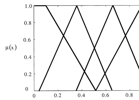
A membership function is a description of the possible states of a descriptor. We assume that each descriptor has the possibility of falling into four alternative states:&low',&moderately low',&moderately high'and&high'. We let the possible states of each market descriptor be represented by a set of four membership functions that are associated with a speci"c shape. The state&low'is associated with a trapezoidal shaped membership function that has its southwest corner at the origin. The state &moderately low' is associated with a triangular shaped membership function that has a base stretching from a point slightly greater than 0 to a point slightly greater than 0.6. The state &moderately high'is also associated with a triangular membership function, but its base runs from a point slightly less than 0.4 to a point slightly less than 1. Finally the state &high' is associated with a trapezoidal membership function that has its southeast corner at the point 1 on thex-axis.16The shapes and locations of these fuzzy sets along the speci"ed range [0, 1] (universe of discourse) are as illustrated in Fig. 1. We represent fuzzy information with the codes&1',&2', &3' and&4' for&low', &moder-ately low',&moderately high'and&high', respectively. A&0'is used to record the absence of a fuzzy set.
An example will help at this point. If the conditional part of the rule is coded as [0 1 3 0 2], this would mean thatp*r/dandp/MA(100) are not present in the conditional part of the rule, that is, the rule assigns no in#uence to these descriptors. In contrastp/MA(5),p/MA(10) andp/MA(500) all have an in#uence and the coding indicates that p/MA(5) is&low',p/MA(10) is&moderately high' andp/MA(500) is&moderately low'. In other words, this corresponds to a state in
which the market price is less thanMA(5) but somewhat greater thanMA(10) and
Fig. 1. Fuzzy sets for the states of the market descriptors.
18These intervals are chosen so that the REE (homogeneous rational expectation equilibrium) values for the market characterized are centered in these intervals.
A critical point to remember is that while these market descriptors are intrinsically fuzzy, the conditions described by them are likely to match many di!erent market situations. What really matters however, is the degree to which each of these conditions is ful"lled and not so much whether each condition is indeed matched or not matched by the prevailing market situation.
3.3.4. Identifying expectation model parameters
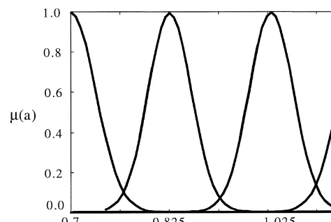
Now we turn to the modeling of the forecast part of the rule. We allow the possible states of each forecast parameter to be represented by four fuzzy sets.
These fuzzy sets are labeled respectively (with the shapes indicated), &low'
(reverse S-curve), &moderately low' (Gaussian-bell curve), &moderately high' (Gaussian-bell curve), and &high' (S-curve). The universe of discourse for the
parameters, aand b are set to [0.7, 1.2] and [!10, 19], respectively.18 The
shapes and locations of the fuzzy membership functions for a and b are as
illustrated in Figs. 2 and 3. When we represent these fuzzy sets as bits, we code them&1',&2',&3', and&4'for&low',&moderately low',&moderately high', and&high' respectively.
Fig. 2. Fuzzy sets for the forecast parameter&a'.
Fig. 3. Fuzzy sets for the forecast parameters&b'.
forecast parameters, we obtain a complete rule which we would code as: [0 1 3 0 2D2 4]. In general, we can write a rule as: [x
1,x2,x3,x4,x5Dy1,y2],
where x
1,x2,x3,x4,x53 M0, 1, 2, 3, 4N and y1,y23 M1, 2, 3, 4N. We would
therefore interpret the rule [x
1,x2,x3,x4,x5Dy1,y2] as:
Ifp*r/disx1andp/MA(5) isx2andp/MA(10) isx3and
p/MA(100) isx
4andp/MA(500) isx5, thenaisy1andbisy2
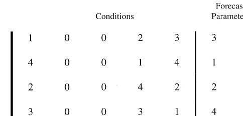
Fig. 4. A complete and consistent rule base.
19It is important to point out that conventional Boolean logic, unlike fuzzy logic, cannot tolerate inconsistencies. For instance, consider the problem of classifying whether someone is tall or short. Boolean logic requires that one de"ne a crisp cut-o!height to separate tall people from short people. So when using Boolean logic, if a person is tall, this person cannot be short at the same time. Fuzzy logic on the other hand allows us to classify a person as belonging to both the fuzzy set of tall and short people. As the reader can see from Figs. 1}3, there is no clear cut-o!for a fuzzy set; it is therefore quite conceivable for the above to happen. In fact, it is this#exibility that allows us not only to better describe things but also to do so in an economical fashion.
3.3.5. Fuzzy rule bases as market hypotheses
A genetic-fuzzy classi"er contains a set of fuzzy rules that jointly determine what the price expectations should be for a given state of the market. We call a set of rules a rule base. Each rule base represents a tentative hypothesis about the market and re#ects a&complete'belief. This point needs further clari"cation. Suppose the fuzzy rule is&Ifp*r/dis high thenais lowandbis high'. This rule
by itself does not make much sense as an hypothesis because it does not specify what the forecast parameters should be for the remaining contingencies, for example the case where p*r/dis &low', &moderately low' or &moderately high'. Three additional rules are therefore required to form a complete set of beliefs.
For this reason, each rule base contains four fuzzy rules.19 Fig. 4 shows an
example of a rule base, coded as a set of four 7-bit strings. This rule base quali"es as a&complete'belief.
We allow each agent in our model to work in parallel with several distinct rule bases. In order to keep the model manageable yet maintain the spirit of competing rule bases, we allow each agent to work with a total of"ve rule bases.
Therefore, at any given moment, agents may entertain up to "ve di!erent
accuracy of the rule bases and acts on the one that has recently proven to be the most accurate. This is the same set up used in the SFASM.
In a separate experiment, we deviate from this strictly deterministic choice system and allow agents to sometimes select the rule base to use in a probabilis-tic manner. The timing of this alternative choice framework is triggered by a random event. Our interest in this modi"cation is motivated by the extensive literature on group polarization, a well-documented phenomenon (for instance, Lamm and Myers, 1978). Shiller (1989, Chapter 2) in a review of group polariza-tion phenomena has suggested that the polarizapolariza-tion of negative attitudes by a group may be triggered by speci"c events. We think of these negative attitudes as &doubts' about whether the perceived best rule base, as measured by its current forecast accuracy, is actually best. We allow such doubts to arise probabilistically, but with a very low probability of occurrence. If the state &doubt'occurs, we tie the probability of selecting a rule base from the"ve held by an investor at the time, to its relative forecast accuracy so the one which has proven to be the most accurate will have the highest likelihood of being selected. However, when doubt prevails, no rule base will be selected with certainty. In other words, we are assuming that agents will sometimes lose con"dence in their best forecasting model, and in those instances they will utilize their second-best or third-best models, etc. This modi"cation is in fact a key extension of the SFASM framework. We show later that the inclusion of this feature produces return kurtosis measures that are more in line with observed data than those produced under the model structure analyzed by LeBaron et al. (1999), while simultaneously generating return and volume behavior that are otherwise similar to actual data.
3.3.6. An example
We now turn to an example of how the fuzzy system operates. Consider a simple fuzzy rule base with the following four rules.
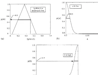
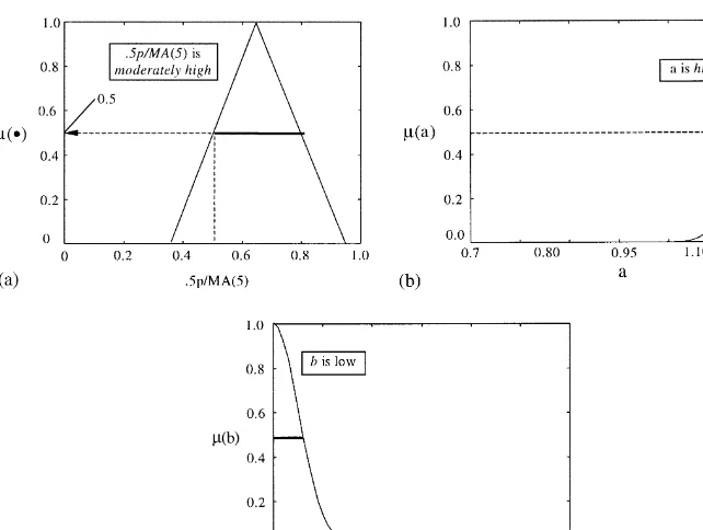
If 0.5p/MA(5) islowthenaismoderately highandbismoderately high. If 0.5p/MA(5) ismoderately lowthenaislowandbishigh.
If 0.5p/MA(5) ishighthenaismoderately lowandbismoderately low. If 0.5p/MA(5) ismoderately highthenaishighandbislow.
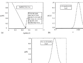
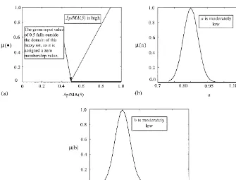
Now suppose that the current state in the market is given byp"100,d"10, and MA(5)"100. This gives us, 0.5p/MA(5)"0.5. The response of each rule and the resultant fuzzy sets for the two forecast parameters, given this state of the market, are illustrated in Figs. 5}10. In particular, note the responses for the 1st and 3rd rules. In these cases, the membership value for those fuzzy sets representing 0.5p/MA(5) is zero since 0.5 is outside their domains, consequently the forecast parameters associated with these rules will also have zero member-ship values. Thus, only the 2nd and 4th rules contribute to the resultant fuzzy
Fig. 5. Response of 1st rule of example rule base to parameter 0.5p/MA(5)"0.5.
20In the centroid method, which is sometimes called the center of area method, the defuzz"ed value is de"ned as the value within the range of variablexfor which the area under the graph of membership functionMis divided into two equal sub-areas (Klir and Yaur, 1995).
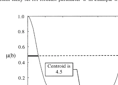
translated into speci"c values foraandb. We employ the centroid method to accomplish this. This amounts to calculating the centroid of the enclosed areas in Figs. 9 and 10.20We&defuzzify'these resultant fuzzy sets using the centroid method, obtaining 0.95 and 4.5 for the parameters&a' and&b', respectively, as shown in Figs. 9 and 10. Substituting these forecast parameters into Eq. (4) gives us the forecast for the next period price and dividend of: E (p#d)"0.95(100#10)#4.5"109.
3.3.7. Forecast accuracy andxtnessvalues
Following LeBaron et al. (1999), we measure forecast accuracy for a rule base by the inverse ofe2
t,i,j. The variablee2t,i,j is the moving average of the squared
forecast error and is de"ned as:
e2
Fig. 6. Response of 2nd rule of example rule base to parameter 0.5p/MA(5)"0.5.
wherehis a constant weight, subscriptiandjdenote theith individual and the jth rule base, andtindexes time. In each period the agents refer toe2t,i,j when deciding which rule base to rely on.
The variablee2
t,i,j is also used for several other purposes. First it is used by
agentias a proxy for the forecast variancep2
t,i,j when setting demand. Second,
the value fore2
t,i,j is used to compute what we will label a"tness measure. In the
experiments, agents revise their rule bases on average everykperiods.
Opera-tionally, this means that the GA is invoked every k periods. The "tness
measure is used to guide the selection of rule bases for&crossover'and&mutation' in the GA. A GA creates new rule bases by&mutating'the values in the rule base
array, or by &crossover' * combining part of one rule base array with the
complementary part of another. In general, rule bases that"t the data well, will
be more likely to reproduce whereas less "t rule bases will have a higher
probability of being eliminated. The"tness measure of a rule base is calculated as follows:
f
Fig. 7. Response of 3rd rule of example rule base to parameter 0.5p/MA(5)"0.5.
21A similar speci"cation is employed by LeBaron et al. (1999).
Fig. 8. Response of 4th rule of example rule base to parameter 0.5p/MA(5)"0.5.
22We mentioned earlier in Section 3.3.5 that a separate experiment involved the introduction of a state of&doubt'in which the rule base choice is probabilistic versus deterministic as described here.
3.3.8. Recapitulation
The model begins with a dividend,d
t, announced publicly at time periodt.
Based on this information, the "ve market descriptors [p*r/d, p/MA(5), p/MA(10),p/MA(100), andp/MA(500)] are computed and the forecast models parameters identi"ed. Agents then generate several di!erent price expectations using their genetic-fuzzy classi"ers. They forecast next period's price and divi-dend (E
i,t[pt`1#dt`1]) by using the forecast parameters from the rule base
that has proven to be the most accurate recently.22With this expectation and its variance, they use Eq. (2) to calculate their desired share holdings. The market
clearing price is then determined att as if by a tatonement process. Once the
market clears, the price and dividend at timetare revealed and the accuracies of the rule bases are updated.
Fig. 9. Resultant fuzzy set for forecast parameter&a'in example where 0.5p/MA(5)"0.5.
Fig. 10. Resultant fuzzy set for forecast parameter&b'in example where 0.5p/MA(5)"0.5. discover which rule bases are accurate and worth acting upon and which should be ignored. At a deeper level, learning occurs at a slower pace as the GA discards unreliable rule bases to make room for new ones through crossover and mutation. The new, untested rule bases that are created will not cause disrup-tions because they will be acted upon only if they prove to be accurate. This avoids brittleness and provides what machine-learning theorists call &graceful-ness' in the learning process.
3.4. Experiments
23The model was coded using MATLAB, a product of the MathWorks, Inc.
behavior of prices and volume in a dynamic setting. In these experiments, we kept almost all of the model's parameters the same so that comparisons can be made of the market outcomes under identical conditions with only controlled
changes.23 The primary control parameter, as in LeBaron et al. (1999), is the
learning frequency constant,k.
Learning frequency refers to the frequency at which a GA is invoked in the model. When the learning frequency is high, a GA is invoked more frequently and agents will revise their rule bases more often. In contrast, when the learning frequency is low, a GA is invoked less often, so agents will revise their rule bases at a slower pace. Recall that agents are not able to use deductive reasoning to shape their price expectations. Instead, they use inductive reasoning which basically amounts to formulating tentative hypotheses and testing these hy-potheses repeatedly against observed data. Under such a scheme, it is clear that the learning frequency will play a key role in determining the structure of the rule bases and how well agents are able to coordinate their price expectations. When learning frequency is high, agents will revise their beliefs frequently so they will typically not have adequate time to fully explore whether their market hypotheses are consistent with those belonging to other agents. At the same time, if agents revise their hypotheses frequently, their hypotheses are more likely to be in#uenced by transient behavior in the time series of market variables. These factors together will make it di$cult for agents to converge on an equilibrium price expectation. In contrast, when learning frequency is low, agents will have more time between revising their rule bases to explore their hypotheses. Furthermore, their hypotheses will also tend to be based on longer horizon features in the time series of market variables. Consequently, agents are more likely to converge on an equilibrium price expectation.
The model's parameters that are common to all the experiments are tabulated
in Table 1. We conducted three sets of experiments. In the "rst and second
experiments, the learning frequency,k, is equal to 200 and 1000, respectively.
This means that the agents learn on average once every 200 time periods in the "rst experiment and once every 1000 periods in the second experiment. In both these experiments, we assume that the agents always form their forecasts using the most accurate rule base.
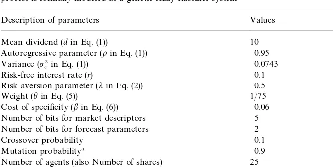
Table 1 Parameter values
Common parameter values in the simulations of an arti"cial stock market in which a risky security is traded and investors are expected utility of"nal wealth maximizers. Investors represented in the model employ induction and reason as if by fuzzy logic when forming their expectations. The process is formally modeled as a genetic-fuzzy classi"er system
Description of parameters Values
Mean dividend (dM in Eq. (1)) 10
Autoregressive parameter (oin Eq. (1)) 0.95
Variance (p2e in Eq. (1)) 0.0743
Risk-free interest rate (r) 0.1
Risk aversion parameter (jin Eq. (2)) 0.5
Weight (hin Eq. (5)) 1/75
Cost of speci"city (bin Eq. (6)) 0.06
Number of bits for market descriptors 5
Number of bits for forecast parameters 2
Crossover probability 0.1
Mutation probability! 0.9
Number of agents (also Number of shares) 25
Number of rule bases per agent 5
Number of fuzzy rules per rule base 4
!This is the probability that an agent will have one of his rule bases subjected to mutation. When a particular rule base is selected for mutation, the probability that each bit is mutated is 0.03, and the probability that a bit will be transformed from 0's to non-0's or vice versa is 0.5.
24Recognize that while a polarization of attitudes can arise with respect to doubt about which of their"ve rule bases is best, the framework we analyze would assign the same"ve rule bases to any two agents only by chance.
when one agent decides to do so, we assume that all the remaining agents follow his example, in other words, a polarization of attitudes arises. In other words, we are assuming that if there is an event that shakes the con"dence of one agent, then the same event will also shake the con"dence of all other agents. The probability that agentiwill select his rule basej(j"1, 2,2, 5) is then linked to the relative forecast accuracy of the rule base. Speci"cally, when a state of doubt arises, we rank the"ve rule bases that an agent carries from 0 to 2, in increments of 0.5, and compute the selection probability for each rule base as follows:
P
wherejindexes the jth rule base.24 Note that agents do not decide to choose
the best rule set with some probability when the state of &doubt' occurs. In addition the probability that governs which rule base will be chosen when the above event happens may be unique for each agent. This probability is deter-mined by the ratings each agents has assigned to each of his"ve rule bases.
We follow LeBaron et al. (1999) in referring to the two cases (k"200 and 1000) as&fast learning'and&slow learning'. Learning takes place asynchronously. In other words, not all the agents in the model update their rule bases simultaneously.
We began with a random initial con"guration of rules. We then simulated the market experiment for 100,000 periods to allow any asymptotic behavior to emerge. Subsequently, starting with the con"guration attained att"100,000 we simulated an additional 10,000 periods to generate data for the statistical analysis discussed in the next section. We repeated the simulations 10 times under di!erent random seeds to facilitate the analysis of regularities that emerge from repeated observation of a complete market realization.
4. Results
Simulation results from our experiments show that the model is able to generate behaviors that bear a strong resemblance to many of the regularities that have been observed in real"nancial markets. We discuss these results in the following sections. Throughout our discussion, the mnemonic REE will stand for Rational Expectations Equilibrium.
4.1. Asset prices and returns
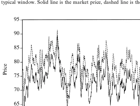
Fig. 11. Experiment 1: slow learning,k"1000. Time series record of the market price and the REE price over a typical window. Solid line is the market price, dashed line is the REE price.
Fig. 12. Experiment 2: fast learning,k"200. Time series record of the market price and the REE price over a typical window. Solid line is the market price, dashed line is the REE price.
Further evidence on the relation between the price level and price variability appears in Table 2. We compute the mean and standard deviation for the market price across the 10 complete market realizations for the three sets of
Fig. 13. Experiment 3: fast learning with doubt,k"200. Time series record of the market price and the REE price over a typical window. Solid line is the market price, dashed line is the REE price.
25For evidence on volatility of market price and related tests, see Leroy and Porter (1981a, b) and Shiller (1981). Shiller (1988) is a discussion of the volatility debate.
26Note thatp2p`d"(1#f)2p2
e"[o/(1#r!o)]2p2e. This result is derived in Appendix A. This equation will give us a variance of 4 for the parameter values listed in Table 1.
estimate the standard deviation for the REE price to be equal to 5.4409. Judging from the standard deviations reported in Table 2, it is clear that the market price in all three sets of experiment is more volatile than the REE price, and that the mean price falls as variability rises.25The larger volatility in the fast learning case (k"200) can be attributed to the more frequent revision of rules by agents. The rules in the fast learning case are also more likely to be based on transient shorter horizon features in the time series of market variables. Agents therefore "nd it necessary to employ di!erent rule bases to form their expectations at di!erent times. This regular switching in the agents'beliefs, in turn, can give rise to higher volatility because they need time to adapt to the changes.
The remaining rows in Table 2, except the last, present results on the behavior of the residual series (e
t) obtained from the following regression equation:
p
t`1#dt`1"a#b(pt#dt)#et`1. (8)
Table 2
Summary statistics for prices, model residuals and implied returns computed from simulations of an arti"cial stock market in which agents form expectations based upon a genetic-fuzzy classi"er system. Experiment 1 involves slow learning. Experiments 2 and 3 involve fast learning!
Variables Experiment 1 Experiment 2 Experiment 3
(slow learning,
Mean (PM) 76.0155 73.5214 69.5040
Std. Dev. (pP) 6.0967 6.6333 7.0422
1(et) (0.0551)0.0102 (0.0589)0.0271 !0.1391(0.0903) o
1(e2t) (0.0177)0.0351 (0.0149)0.0427 (0.0874)0.324
ARCH LM(1)# 15.1822 20.3300 1104.2077
[0.6] [1.0] [1.0]
t) !0.0095(0.0726) (0.0941)0.0734 !0.1038(0.0737)
o
1(R2t) !0.0058(0.0703) (0.1416)0.0948 !0.0685(0.0641)
!This table gives the average of each variable over the 10 simulations conducted for each experiment. The numbers in parentheses are the standard errors. Skewness, kurtosis and"rst-order autocorrelation are computed in the conventional manner (see Greene, 1993).
"Residuals are computed from the modelp
t`1#dt`1"a#b(pt#dt)#et`1.
#The numbers for the ARCH LM(1) tests are the means of theF-statistics for the 10 simulations for each experiment and the numbers in square brackets are the percentage of the number of tests that reject the null hypothesis of&no ARCH'.
Table 3
Summary statistics for the daily with-dividend returns for the common stocks of the Walt Disney Company, Exxon Corporation and IBM Corporation. Data are from the period 01/03/68 through 12/31/98!
Panel B. Daily returns from 01/03/63 to 12/31/98 (excluding the observations from Oct. 19, 1987
through Oct 21, 1987)
!Skewness, kurtosis and"rst-order autocorrelation are computed in the conventional manner (see Greene, 1993).
"Denotes signi"cance at 5% con"dence level.
#Denotes signi"cance at 1% con"dence level.
that the theoretical standard deviation fore(
t should be 2. Furthermore, under
a Gaussian distribution the excess kurtosis of the error should be zero. We compare these theoretical results to those in the third and"fth rows in Table 2. It is apparent from the values in the third row that the residual series from Experiment 3 exhibits more variability than what is implied by the REE solution. The standard deviation of the residual series from Experiments 1 and 2 are slightly larger than 2.
The"fth row shows that the residual series from Experiments 1 and 2 exhibit slightly excess kurtosis. But, the kurtosis from Experiment 3 is much larger than these two and the magnitude is consistent with that of the daily common stock returns presented in Table 3. Table 3 presents summary statistics for the daily with-dividend returns of three common stocks: Disney, Exxon, and IBM. The data span the period 1/03/63}12/31/98 and are from the CRSP Daily Stock Return File. Our model is capable of creating market crashes like what we have
seen in actual "nancial markets. We have excluded those simulations that
27When we included those simulations that contain market crashes in the summary calculations, the mean kurtosis became 24.7239 which is consistent with the result in the top panel in Table 3. Table 2. Therefore, to facilitate comparison, we have presented the summary statistics for the actual data for two separate data sets. The top panel of Table 3 includes observations from the 1987 market crash and the bottom panel ex-cludes these same observations. It is clear that the kurtosis we have generated is consistent with the descriptive statistics presented in the lower panel of
Table 3.27As mentioned earlier, we began each simulation with a random initial
con"guration of rule bases. What we observed during the course of each simulation was that kurtosis is always rather large during the"rst few hundred time steps (usually up to roughly 1000 time steps) during which the agents' learning curves are the steepest. The agents in the model have the unenviable task during the early phase of the simulation of"guring out how to coordinate their expectations by sorting out the rules that work from the many arbitrary rules they have been endowed with. However, once the agents have identi"ed rule bases that seem to work well, excess kurtosis decreases rapidly until it is almost equal to zero. From that point on, it is extremely di$cult (but not impossible) for the model to generate further excess kurtosis without some exogenous perturbation. We may observe spurts of excess kurtosis arising from a substantial sudden change in the mind of the agents as a whole, such as in the case of an emerging trend, although this is rare. In such a case, the excess kurtosis usually lasts for a short time and such infrequent events are easily washed out when we consider a long return series, except in the presence of a large price deviation.
We conclude that the reason it is so di$cult to generate large kurtosis (without relying on an exogenous perturbation) is because it is di$cult to break the coordination among the agents in the model once they have established some form of mutual understanding. This is in fact consistent with received wisdom. In actual stock markets, price swings are often triggered by exogenous events (such as rumors or earnings surprises) which are then perpetuated by endogenous interactions among traders. We suspect the large kurtosis observed in actual returns series may have originated from such exogenous events. It is in this spirit that we introduced what we earlier referred to as a state of&doubt'.
The sixth row in Table 2 presents statistics on the autocorrelation in the residuals from Eq. (8). The autocorrelation coe$cients tell us whether there is any linear structure remaining in the residuals. Other than the result for Experiment 3, the results for the"rst two experiments show that there is little autocorrelation in the residuals. This corresponds to the low actual autocorrela-tions shown in Table 3.
28Unlike LeBaron et al. (1999), we have not placed an upper bound on the number of shares that can be traded by any single agent, in particular we impose no short sale restriction.
29See Karpov (1987).
1992; Glosten et al., 1994; Nelson, 1991). We test for ARCH dependence in the residuals and present the results in Rows 7 and 8 of Table 2. We test for ARCH e!ects in two di!erent ways. In Row 7, we present the"rst order autocorrelation of the squared residuals. In Row 8, we perform the ARCH LM test proposed by Engle (1982). Both of these tests reveal that there is ARCH dependence in the residuals. However, the e!ect is more pronounced for the two fast learning cases.
In these two experiments we rejected the null hypothesis of&no ARCH'at the
95% con"dence level for all 20 simulations using the ARCH LM tests. The null was rejected for only 6 of the simulations in the slow learning casel.
We also computed statistics for the returns based upon the simulated prices and dividends. These statistics appear as the"nal"ve rows of Table 2. Now comparing Tables 2 and 3 we see that the correspondence between the returns computed from the simulated data, and the actual return data are even more striking. The standard deviation, skewness as well as kurtosis statistics for the simulated returns from experiment 3 are very similar to those shown for the stocks in Table 3.
4.2. Tradingvolume
Figs. 14 and 15 present snapshots of observed trading volume over a typical window for both the fast-learning and slow-learning cases. Trading is active,
consistent with real markets. In fact, we "nd that the volume of trade in
Experiment 3, on occasion, can exceed 50% of the total number of shares available in the market. In both Experiments 1 and 2, the volume of trade can be
as high as 33%.28The summary statistics for trading volume are presented in
Table 4.
Figs. 16}18 plot the volume autocorrelations for both the fast-learning and slow-learning experiments. In these three plots, the broken lines are one stan-dard deviation away from the continuous line, which is the mean of the autocorrelations computed for each of the 10 experiments for each case. These plots show that trading volume is autocorrelated. This result lines up well with the positive autocorrelations usually found in time series of the volume traded
for common stocks.29Fig. 19 shows a plot of the daily volume autocorrelations
for Disney, Exxon, and IBM. Figs. 16}18 show that the model produces volume autocorrelation behavior strikingly similar to what is observed for the actual data presented in Fig. 19.
Fig. 14. Experiment 1: slow learning,k"1000. Time series record of the volume of shares traded over a typical window.
Fig. 15. Experiments 2 and 3: fast learning and fast learning with doubt,k"200. Time series record of the volume of shares traded over a typical window.
Table 4
Summary statistics for volume of trading per time step computed from simulations of an arti"cial stock market in which agents form expectations based upon a genetic-fuzzy classi"er system. Experiment 1 involves slow learning. Experiments 2 and 3 involve fast learning. Summary statistics are based upon 10 simulations of each experiment
Variables Experiment 1 Experiment 2 Experiment 3
(slow learning,
k"1000)
(fast learning,
k"200)
(fast learning with doubt,k"200)
Mean! 0.7346 0.8196 0.9369
Maximum" 7.2514 8.2833 12.5978
Minimum" 0.0225 0.0322 0.0203
!Grand mean per time step over all simulations for a given experiment.
"Maximum (Minimum) per time step over all simulations for a given experiment.
Fig. 16. Experiment 1: slow learning,k"1000. Volume autocorrelations measured at various lags.
Fig. 17. Experiment 2: fast learning,k"200. Volume autocorrelations measured at various lags.
Fig. 19. Sample daily volume autocorrelations for the common stocks of Disney, Exxon and IBM.
Fig. 21. Sample crosscorrelations between squared daily returns at (t#j) and volume attfor the common stocks of Disney, Exxon and IBM.
30This result lends support to our assumption that Eq. (2) describes individual demands. Despite the fact that prices during periods that track the REE solutions are not normally distributed, market clearing prices based upon demands as given by (2) give the correct values after accounting for the additional variability in the system due to learning.
4.3. Market ezciency
Fig. 22 plots a snapshot of the di!erence between the REE price and the market price over a typical window. This plot displays periods during which the
market price is highly correlated with the REE price.30 However, there are
periods of sporadic wild#uctuations during which this relation is broken. We
Fig. 22. Experiments 2 and 3: fast learning and fast learning with doubt,k"200. The time series record of the di!erence between the market price and the REE price over a representative window. Experiment 2: top line; Experiment 3: bottom line.
31The DJIA closed at 7715.41 on Friday, October 24, 1997. The close on Monday, October 27, 1997 was 7161.15. This was in turn followed by it closing on Tuesday, October 28 at 7498.32. This sequence of outcomes was not peculiar to the DJIA as most other major market indices also experience major changes.
This type of behavior is not uncommon in real "nancial markets. The
historical record suggests that most of the time, prices of "nancial securities appear to be set in an e$cient fashion. However, there have been occasions during which prices depart and appear to exhibit a behavior unrelated to fundamentals. This is especially evident during those periods that most ob-servers would classify as either bubbles or crashes. A good example is the change that occurred on October 27, 1997. On that day the Dow
Jones Industrial Average dropped 554.26 points.31The peculiar fact is not the
5. Conclusions
This paper argues that many of the regularities observed in common stock returns can be explained by allowing agents in otherwise traditional asset market models to form their expectations in a manner akin to how investors would form their expectations in real life. In particular, because the environment that investors operate in is ill-de"ned, they will have to rely on their innate abilities to analyze in fuzzy terms and reason inductively. We show that these traits can be faithfully captured by a genetic-fuzzy classi"er system. We sub-sequently assert that models, which endow agents with such a reasoning process, will account for some of the documented empirical puzzles observed in real markets and will generate price and return behavior consistent with actual data. We document a close correspondence between statistics computed from our simulations and statistics computed from actual return series. These include descriptive statistics for returns as well as the resulting behavior of volume autocorrelations and volume and volatility cross-correlations. We show that a basic framework, however, is not capable of generating return kurtosis measures that are consistent with actual data. A modi"cation of the model to allow for the intrusion of a (low probability) state of&doubt'about what would otherwise have been identi"ed as the best prediction rule, is shown to produce return kurtosis measures that are more in line with actual data.
Summing up, our model can account simultaneously for several regularities observed in real markets, that have been a struggle to rationalize within the context of the traditional rational expectations paradigm. First, our model can give rise to active trading. Second, our model supports the views of both academicians and market traders. Academic theorists in general view the market as rational and e$cient. Market traders typically see the market as psychologi-cal and imperfectly e$cient. In our model, we"nd that the market moves in and
out of various states of e$ciency. Furthermore, we "nd that when learning
occurs slowly, the market can approach the e$ciency of a REE. Finally, descriptive statistics for the returns implied by the simulated price and dividend series are shown to be consistent with results for actual data, as are the results for volume and volatility.
logic. Our agents therefore work with only a handful of rule bases, but these have the special characteristic that they are fuzzy rules. Our agents still modify their rules using induction (modeled by a genetic learning system), but accomplish the same objectives as the model of LeBaron et al. with a much smaller set of rules. The fact that a model based upon a fuzzy system generates market behavior similar to a model based upon crisp but numerous rules is appealing because fuzzy decision making has appeal as a reasonable attribute for individuals.
Acknowledgements
The authors are grateful to an anonymous referee and the editor, Leigh Tesfatsion, for their comments and suggestions, and to Gary Emery, Jim Horrell, Bryan Stanhouse, and Zhen Zhu, for their comments on an earlier version of the paper. Linn gratefully acknowledges support from the Ronn Lytle Summer Research Grant Program in the Price College of Business at the University of Oklahoma.
Appendix A. Solution for a linear homogeneous rational expectations equilibrium of the model
The dividend process and the demand for the security as delineated in the text are given by
We assume that agents conjecture that price is a linear function of the dividend, that is,
p
t"f dt#e.
In equilibrium, each agent must hold the same number of shares (since all the agents are equally risk averse). Given that the total number of shares is equal to the total number of agents, each agent must hold only one share at all times in equilibrium. This allows us to set the demand equation to one. We can then substitute the above expression for the one-period ahead forecast into the demand equation to obtain,
The LHS of this expression is a constant. Therefore, the RHS cannot exhibit any
dependence on time. So terms containingd
t must vanish. This leads to
(1#f)o!(1#r)f"0,
f" o (1#r!o).
The quantity &e' can be obtained by substituting f back into the demand
equation and setting demand equal to 1, yielding
e"dM(f
#1)(1!o)!jp2
p`d
r .
The relationship between the forecast parameters&a'and&b'in our model and the REE parameters can now be established. We"rst write the one-period ahead optimal forecast for price and dividend as
E(p
t`1#dt`1)"o(pt#dt)#(1!o)[(1#f)dM#e].
Comparing this equation to E(p
t`1#dt`1)"a(pt#dt)#b, gives
a"o,
b"(1!o)[(1#f)dM#e].
References
Arthur, W.B., 1991. Designing economic agents that act like human agents: a behavioral approach to bounded rationality. American Economic Review 81, 353}359.
Arthur, W.B.,1992. On learning and adaptation in the economy. Working Paper 92-07-038, Santa Fe Institute.
Arthur, W.B., 1994. Inductive reasoning and bounded rationality. American Economic Review 84, 406}411.
Arthur, W.B., 1995. Complexity in economic and"nancial markets. Complexity 1, 20}25. Arthur, W.B., Holland, J.H., LeBaron, B., Palmer, R., Taylor, P., 1997. Asset pricing under
Black, F., 1986. Noise. Journal of Finance 41, 529}544.
Blume, L.E., Easley, D., 1995. What has the rational learning literature taught us? In: Kirman, A., Salmon, M. (Eds.), Learning and Rationality in Economics. Basil Blackwell, Cambridge. Bollerslev, T., 1986. Generalized autoregressive conditional heteroskedasticity. Journal of
Econometrics 31, 307}327.
Bollerslev, T., Chou, R.Y., Kroner, K.F., 1992. ARCH modeling in"nance: a review of the theory and empirical evidence. Journal of Econometrics 52, 5}59.
Bray, M.M., 1982. Learning, estimation and the stability of rational expectations. Journal of Economic Theory 26, 318}339.
Brock, W.A., Hommes, C.A., 1998. Heterogeneous beliefs and routes to chaos in a simple asset pricing model. Journal of Economic Dynamics & Control 22, 1235}1274.
De Long, J.B., Shleifer, A., Summers, L.H., Waldman, R.J., 1989. The size and incidence of the losses from noise trading. Journal of Finance 44, 681}696.
De Long, J.B., Shleifer, A., Summers, L.H., Waldmann, R.J., 1990. Positive feedback investment strategies and destabilizing rational speculation. Journal of Finance 45, 379}396.
Dreman, D., 1977. Psychology and the Stock Market: Investment Strategy Beyond Random Walk. Amaco, New York, NY.
Dreman, D., 1982. The New Contrarian Investment Strategy. Random House, New York, NY. Engle, R.F., 1982. Autoregressive conditional heteroskedasticity with estimates of the variance of
United Kingdom in#ation. Econometrica 50, 987}1007.
Gennotte, G., Leland, H., 1990. Market liquidity, hedging and crashes. American Economic Review 80, 999}1021.
Glosten, L.R., Jagannathan, R., Runkle, D., 1994. Relationship between the expected value and the volatility of the nominal excess return on stocks. Journal of Finance 48, 1779}1801.
Goldberg, D.E., 1989. Genetic Algorithms in Search, Optimization and Machine Learning. Addison-Wesley, Reading, MA.
Greene, W.H., 1993. Econometric Analysis. Macmillan, New York, NY.
Grossman, S.J., 1976. On the e$ciency of competitive stock markets where traders have diverse information. Journal of Finance 31, 573}585.
Holland, J.H., Holyoak, K.J., Nisbett, R.E., Thagard, P.R., 1986. Induction: Processes of Inference, Learning, and Discovery. MIT Press, Cambridge, MA.
Holland, J.H., Reitman, J., 1978. Cognitive systems based on adaptive algorithms. In: Waterman, D.A., Hayes-Roth, F. (Eds.), Pattern-Directed Inference Systems. Academic Press, New York, NY. Jacklin, C.J., Kleidon, A.W., P#eiderer, P., 1992. Under estimation of portfolio insurance and the
crash of October 1987. Review of Financial Studies 5, 35}63.
Karpov, J.M., 1987. The relation between price changes and trading volume: a survey. Journal of Financial and Quantitative Analysis 22, 109}126.
Keynes, J.M., 1936. The General Theory of Employment, Interest and Money. Macmillan, London. Klir, G.J., Yaur, B., 1995. Fuzzy Sets and Fuzzy Logic: Theory and Applications. Prentice Hall,
Englewood Cli!s, NJ.
Lamm, H., Myers, D.G., 1978. Group-induced polarization of attitudes and behavior. In: Berkowitz, L. (Ed.), Advances in Experimental Social Psychology, Vol. 11. Academic Press, New York, NY.
LeBaron, B., 2000. Agent based computational "nance: suggested readings and early research. Journal of Economic Dynamics & Control, 24, 679}702.
LeBaron, B., Arthur, W.B., Palmer, R., 1999. Time series properties of an arti"cial stock market. Journal of Economic Dynamics & Control 23, 1487}1516.
Leroy, S.F., Porter, R.D., 1981a. Stock price volatility: tests based on implied variance bounds. Econometrica 49, 97}113.