Vol. 44 (2001) 201–219
Why do black basketball players
work more for less money?
Robert E. McCormick
a, Robert D. Tollison
b,∗aDepartment of Economics, Clemson University, Clemson, SC 29631, USA bSchool of Business, University of Mississippi, University, MS 38677, USA
Received 1 November 1998; received in revised form 23 March 1999; accepted 31 March 1999
Abstract
We explore Kahn and Sherer’s finding that National Basketball Association players’ salaries are lower for black than white players. In general, we do not find evidence that this salary differential is due to the racial preferences of fans. Specifically, we observe that black players actually play more than comparable white players. We offer a theory of price discrimination based on relative supplies and supply elasticities, in lieu of the racial discrimination argument, as an explanation for the black/white wage differential. © 2001 Elsevier Science B.V. All rights reserved.
JEL classification: J15
Keywords: Wage differential; Customer discrimination; Price discrimination
1. Introduction
The literature on the economics of sports has demonstrated that sports data and organiza-tions provide a useful and accurate laboratory for the study of some economic issues (Goff and Tollison, 1990). Nonetheless, the enduring value of the economics of sports lies in its ability not just to understand the play of sports, but to improve our understanding of general economic problems. Take the problem of racial discrimination. There is a well developed literature on this general issue, but a host of questions remain for researchers. For instance, Kahn and Sherer (1988) presented evidence that black professional basketball players are
∗Corresponding author. Tel.:+1-601-232-5041; fax:+1-601-232-5821. E-mail address: [email protected] (R.D. Tollison).
compensated as much as 20 percent less than white players with comparable skills.1 They explained this differential by appeal to an argument about customer discrimination by Na-tional Basketball Association (NBA) fans, which they test and find not to be refuted for six seasons worth of data on NBA attendance. In other words, NBA fans prefer to see more white players, all else the same. Kahn and Sherer estimated that an additional white player of equal skills increased home attendance by some 8000–13,000 fans per season. At an av-erage ticket price (plus concession revenues) of US$12, the revenue effect of the additional white player more than outweighs the estimated salary differential, suggesting that team owners and white players share in the gains from satisfying customer preferences for white players.2
While Kahn and Sherer present an interesting thesis, it has not been carefully compared with alternative explanations of pay differentials. This is the problem tackled here. Indeed, when all is said and done, the expression “racial discrimination” is very confusing. More precisely, is there a theoretical distinction between racial and price discrimination? If so, what does it mean? In the classical model of third-degree price discrimination, a single-price seller (or in this case buyer) separates the market into two or more submarkets based on some easily identifiable characteristic, for example, foreign or domestic buyers. If these sub-markets have different elasticities of demand (or supply), and if recontracting is costly (and if the antitrust authorities can be kept at bay), a profit opportunity arises. The buyer reduces the consumption of the relatively inelastically supplied input and increases consumption of the (homogeneous) elastically supplied input.
Few have any trouble with this model with minor exceptions.3But the real issue involves the question, if the market happens to be separated on the basis of race, but solely for purposes of price discrimination, is that what one wants to call racial discrimination? Put differently, if race or skin color reveal information about a buyer’s (or seller’s) idiosyncratic elasticity of demand (or supply), should this characteristic be called racial or should the issue more appropriately focus on the underlying reasons why there is a connection between race and elasticity. The normal idea of racial discrimination involves the special treatment of black (or white or yellow or red) people simply because their skin is different without regard to questions of whether their elasticity of demand or supply might be collinear with their skin color. Accepting Kahn and Sherer’s wage-differential result, do black professional basketball players make less money than white players, all else equal, because fans and owners have racial preferences at the margins? That is, do fans or owners simply not like to see black players play? Or, in the alternative, do black professional basketball players earn less money, other things the same, because they belong to a class of identifiable people, who
1Dey (1997) suggests that convergence has taken place and that today there is no racial salary differential. For
additional work in this general area (see Andersen and LaCroix, 1991; Bodvarsson and Brastow (1994); Brown and Jewell, 1995; Brown et al., 1991; Burdekin and Idson, 1991; Hamilton, 1991; Koch and Vander Hill, 1988; Marburger, 1996; Nardinelli and Simon, 1990). Kahn (1991) provides a useful overview.
2NBA revenue sharing does not include live attendance revenues. The home team retains these revenues, less
a stipulated percent charge which goes to support the league office. The NBA shares equally with each team all revenues generated by national television (TV) contracts. Local teams keep virtually all of the TV revenues generated by local TV broadcasts. We note that the sharing rule for national TV revenue mutes the incentive of any team to practice racial discrimination in the first place even if fans are racially biased.
for some currently unknown reason, are not very responsive to wages paid in professional basketball?4
Why is this distinction important? If racial bias provides the explanation of the wage gap, then cultural shifts and education and integration of black people more completely into the culture should reduce the wage gap as the tastes of racially biased fans recede. On the other hand, if fans are not biased, that is, they do not care about the skin color of players, only that they play well and win, the wage gap persists as the society loses its racially segregated attitudes. If price discrimination is the basic reason why black NBA players earn less than white players, the attitude of the fans is irrelevant. Indeed, the extent of the wage gap depends on the relative supply elasticities of black and white players.
This paper explores Kahn and Scherer’s results in search of a better understanding of this issue. We accept their result of a 20 percent salary differential. In an expanded sample of NBA seasons, however, we find no evidence of general customer discrimination by NBA fans. To the contrary, if anything, there is a preference for more black players and more black playing time in our results.5 However, there do appear to be patterns of racial composition across teams in the NBA. We start with the same empirical model as Kahn and Scherer, but add two more seasons’ worth of attendance data.6We identify a pattern of racial preference in NBA cities with large black populations. We also model playing time for NBA players as a function of performance and race. Definitively, black players play more minutes than seemingly comparable white players.
In light of these results, we are left with the following: (a) a large salary differential between black and white players, (b) a weak basis for a claim of general customer dis-crimination, and (c) more playing time for black players, all else equal. This pattern of results, in our view, is suggestive of price discrimination. NBA owners and executives are engaging in price discrimination across classes of players who have different elasticities of supply. For whatever reason (including past racial discrimination), black players have a more unresponsive elasticity of supply with respect to providing professional basketball services than do comparable white players, and hence their salaries can be set lower without erasing their supply of labor. The salary differential identified by Kahn and Scherer is most likely a result of this condition.
2. Monopsony power?
In order for the NBA to price discriminate between player inputs on any basis, the league must face an upward sloping supply curve of labor. We contend that the market for professional basketball talent exhibits this characteristic. Moreover, the rules and institutions of the league must prevent internal competition among teams that would otherwise force
4When there are two different sources of labor in a market, if the elasticities of labor supply are sufficiently
different and the supply of one source, the more elastic one, is larger than the relatively inelastic supply, then the more inelastic workers will work more at lower wages.
5We augment Kahn and Scherer’s use of the number of white players per team with measures of actual playing
time by season for white and black players.
6Their estimates covered the seasons from 1980−1981 through 1985−1986; ours cover the seasons from
Table 1
Home attendance 184 464714 456628 136944 160537 1066505
Ticket price 157 11.37 11.00 2.59 7.00 18.50
Ratio of number of white
Number of all-stars 184 1.011 1 0.986 0 4
individual owners to pay each player the value of his marginal product. We believe that the institutions of the NBA reveal just such a pattern over the time period at issue.
First, there is a draft of players out of the college ranks each year.7 This draft allocates the signing rights for each player chosen to one team for 1 year, thus eliminating any intra-league competition during that year for incoming players. Starting with the 1976–1977 season and carrying through the 1981–1982 season, the collective bargaining agreement (CBA) between the league and its players association allowed for limited free agency. The team bidding away a player had to pay compensation to the player’s team, plus the existing team had the right of first refusal (matching) on any new contract. The CBA that went into effect for the 1982–1983 season maintained limited free agency for players. It eliminated the compensation clause, but retained the right of first refusal. The 1987–1988 season began a new CBA which continued restricted free agency for a player’s first 4 years in the league, and was followed by unrestricted competition among teams for a player’s services after a player had been in the league for 4 years or two contracts.
So even if certain players today face sufficient competition to avoid being discriminated against, the institutions in place for the period of our data, 1980–1988, are sufficient to allow for the exploitation of differences in labor supply among classes of inputs. Until the data on current salaries are available, we cannot investigate whether the wage differential between black and white players persists in this new era of intra-league competition for veteran talent.
3. Attendance results
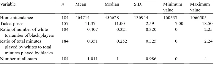
We accumulated data on NBA teams for eight seasons, 1980–1981 through 1987–1988, primarily from various issues of Sporting News Official NBA Guide8 and Sporting News Official NBA Register.9 Summary statistics on these data are reported in Table 1. Over the period of the data, the average team drew slightly less than half-a-million home fans
7Colleges supply the overwhelming bulk of players; occasionally, a foreigner or high school athlete is drafted. 8NBA Guide, 1980–1981 to 1987–1988. The Sporting News, St. Louis.
9We identified the race of each player by examination of his picture in the NBA register. NBA register, 1980–81
for the season. This amounts to 11,334 fans per game. The average ticket price was US$ 11.37, generating slightly more than US$ 5 million in gate receipts per year for regular season games.10 There were about two and a half black players for each white player on the average team.11 But black players play almost three times as many minutes as whites on average. There are 13 cases (out of a possible 184) where the number of whites is equal to or greater than the number of blacks in a team. We note that the predominately white teams are either in Boston or the west depending upon where one places the two Dallas entries.
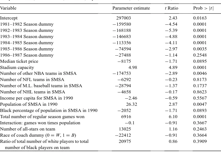
We employ various techniques to investigate the relation between attendance and racial composition. First, we regress NBA home attendance on price and several other demand variables, including the ratio of white to black players.12 The results of estimating the home attendance equation by ordinary least squares are reported in Table 2.13
We note several things about these results. The sport is growing in attendance over time. The first law of demand is not denied. A second NBA team in an SMSA reduces attendance for each team in the area by about 178,000 fans per year. The presence of a National Football League (NFL) or National Hockey League (NHL) team seems to have no impact on basketball attendance, but a major league baseball team is negatively linked to attendance. Bigger populations are associated with more attendance, but there is no link with income. Other things the same, the number of all-stars on a team is not related to attendance.
The relation between winning and attendance is complicated by our inclusion of an in-teraction between winning and population. It has been speculated that the sensitivity of attendance to won–lost records depends on population. The probability that a given fan will attend is a function of record, so that total attendance is the product of this probability and the size of the market. Thus, we interact wins and population. The partial derivative of attendance with respect to winning is:∂attendance/∂wins=6916−0.1×population. The mean population in this sample is 5224. Therefore, at the mean, the relation between games won and attendance is an additional 6394 fans per each additional game won over the season. The maximum SMSA population in our database, New York, is 18,087. There-fore, the relation between winning and attendance is positive over the whole range of the data.
10Each team offers an array of seats and ticket prices. We chose the median ticket price as our measure. Hence,
this average is an average of medians.
11The nuances of the data source do not allow us to measure the racial composition of a team at every moment
in time. The data are season aggregates. Hence, when players are traded or released, we do not observe the exact composition. What we observe is the total number of white and black players that played for a given team at any time during the season.
12We are missing ticket price data for 27 observations. This reduces the sample size from 184 to 157 when this
variable is included.
13Parameter estimates are deductively equivalent using an alternative measure of racial composition, the ratio of
Table 2
OLS regression estimates of NBA home attendance
Sample size: 156; F ratio: 15.95; R2: 0.703; dependent mean: 470,731, root M.S.E.: 81,334
Variable Parameter estimate t Ratio Prob>|t|
Intercept 297003 2.43 0.0163
1981–1982 Season dummy −159580 −4.54 0.0001
1982–1983 Season dummy −168188 −5.39 0.0001
1983–1984 Season dummy −146683 −4.88 0.0001
1984–1985 Season dummy −113356 −4.11 0.0001
1985–1986 Season dummy −74594 −2.97 0.0035
1986–1987 Season dummy −27488 −1.14 0.2548
Median ticket price −8175 −1.71 0.0895
Stadium capacity 4.98 4.89 0.0001
Number of other NBA teams in SMSA −174753 −2.89 0.0046
Number of NFL teams in SMSA −6292 −0.23 0.8173
Number of M.L. baseball teams in SMSA −28794 −1.37 0.1737
Number of NHL teams in SMSA −4658 −0.17 0.8623
Income per capita for SMSA in 1990 −2.46 −0.59 0.5567
Population of SMSA in 1990 26.32 2.87 0.0047
Black percentage of population in SMSA in 1990 −2052 −1.71 0.0893 Total number of regular season games won 6916 6.10 0.0001 Interaction: games won times population −0.1 −0.91 0.3667
Number of all-stars on team 13025 1.16 0.2463
Race of coach dummy (0=W, 1=B) −22412 −0.91 0.3664 Ratio of total number of white players to total
number of black players on team
20975 0.86 0.3909
Most importantly, we find no statistically meaningful relation between the racial com-position of the team, as measured by the ratio of the total number of white players to total number of black players on the team, or the ratio of total minutes played by whites to to-tal minutes played by blacks, and home attendance. At least based on these data and this specification, we find no reason to believe that NBA fans are, in general, racially biased.14 This result is bolstered by the absence of a significant relation between the race of the head coach and attendance. Fans do not seem to care much about the race of the coach or the players, other things the same.
We use the (unreported) fixed effects coefficients to investigate the time-series character of intra-city competition among teams. Starting with the 1984–1985 season, the San Diego Clippers moved without league approval to Los Angeles. The dummy coefficient for the Lakers prior to the arrival of the Clippers in Los Angeles is 184,851 fans per season (relative to the Washington Bullets), and 92,671 afterwards. The Lakers are estimated to draw 92,180 fewer fans (about half as many) after the Clippers arrived in town. At the same time the coefficient for the Clippers in San Diego is−30,277 and 25,013 in Los Angeles, an increase of 55,290. The Clipper’s gain is less than the Laker’s loss, a result that may shed light on
14The OLS results from employing a fixed-effects model across cities yields a similar outcome. For instance, the
the league’s desire to control the property rights to team movement to venues where other NBA franchises are located.15
The basic customer discrimination hypothesis does not stand up in these results. Of course, we have not shown that white fans do not prefer white players or that black fans do not prefer black players (or the reverse). Until we can observe the racial composition of those buying tickets, this issue remains open.16
4. Local differences in racial preferences
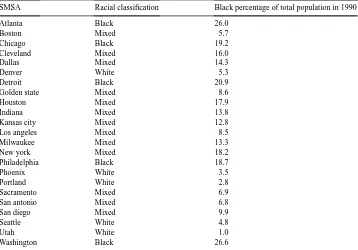
To investigate whether there are regional or local differences in racial preferences, we parse the data into racial groups based on the black percentage of population in the under-lying SMSA. The quartiles of this variable in our sample are 5.7 percent black at the lower end and 18.2 percent at the top end. We define an SMSA as White if it falls in the lower quartile; Black if occurs in the top quarter; and Mixed if it lands in the middle half of the distribution. Table 3 reports the breakdown of the individual SMSAs.
We reestimated the attendance equation allowing for separate coefficients on racial com-position in the three-racial classifications. The results on the racial comcom-position variable, white to black player ratio, are reported in Table 4. We suppress the printing of the other coefficients. They are nearly the same as those reported in Table 2.
This technique reveals that there is a pattern in the relation between team racial com-position and home attendance that seems to depend on the underlying racial comcom-position of the community, a result that was not apparent using the simple black percentage of the population as a control variable. There is no statistically credible relation between the racial composition of the team and attendance in racially mixed or white SMSAs, but there is a relation in the predominately black SMSAs. In the last category, a whiter team is associated with lower attendance. By contrast to the earlier pooled results, we find that there is an attendance relation with team racial composition; the F statistic on the interaction class is 2.72, which is significant at the 5 percent level.17 These results suggest that black fans have a preference for black players in largely black areas, while there is weaker evidence
15The Clippers moved to Los Angeles without the formal approval of the NBA. A litigation ensued which was
ultimately settled out of court.
16There is an endogeniety issue that clouds this result. If the marginal cost of a minute of given player quality is
lower for blacks than whites, relative playing minutes may affect ticket prices, so an OLS regression of demand does not work to estimate the attendance effects of racial composition. To address this question, we estimated the attendance equation jointly with a ticket price equation. The structural ticket price equation has price depending on stadium capacity, year, population, income per capita, and the ratio of white to black players on the team. In the structural estimates, ticket price is positively related to the player ratio variable. However, two-stage estimates of the attendance equation do not alter the previous conclusion about racial composition and attendance. The racial composition variables remain insignificant. The two-stage estimate of the composition coefficient is 8886, and the t ratio is 0.348. The insignificant relation between racial composition and attendance is not blurred by an endogeniety problem.
17This result holds over alternative specifications where we omit the black population variable, and where we
Table 3
The distribution of black population across NBA cities, 1990
SMSA Racial classification Black percentage of total population in 1990
Atlanta Black 26.0
Parameter Estimates on Racial Composition in Attendance Equation Across NBA SMSAsa Sample size: 157; F ratio: 16.29; R2: 0.717
SMSA classification Parameter estimate t Ratio Prob>|t|
Blackest quartile −206074.6 −2.43 0.0165
Mixed half 12874.6 0.52 0.6062
Whitest quartile 39733.4 1.20 0.2333
aThese parameter estimates are the interaction of the SMSA classification and the racial composition variable,
total number of white players divided by total number of black players on a team. The F statistic on the interaction class is 2.72 which is significant at the 5 percent level.
that white fans likewise prefer white players in predominately white areas, all else equal. In the racially mixed areas, no such relation is revealed.18
These results do not provide an explanation for a salary wedge between white and black players. In general, we find no relation between race and attendance. In more detailed examination of NBA venues, we find that black players are sometimes preferred over whites,
18In pairwise tests the coefficient on team racial composition in the blackest quartile is significantly different
and white players are sometimes viewed as better by some fans. Thus, the source of the wage differential identified by Kahn and Sherer remains at issue. Indeed, according to the model of racial discrimination, black players ought to make more money in certain NBA markets than comparable white players.
5. Playing time results
Our basic premise is that what may look like racial/gender/age discrimination is some-times more properly characterized as simple price discrimination. To continue this investi-gation, we now examine whether there is any systematic relation between minutes played and race.
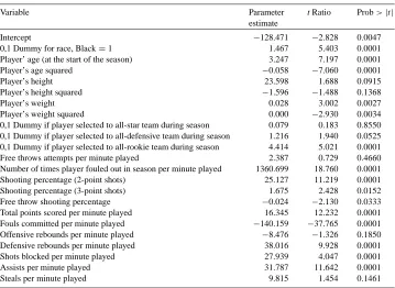
Following other models of playing time, we regress average minutes played per game for each player on each team over the sample period 1980–1981 through 1987–1988 on a vector of player skills (Clement and McCormick, 1989). The dependent variable, average minutes played per game, is total minutes played in a season for each player divided by the number of games that this player participated in during that season.19 We include a dummy for race in this equation to assess whether this factor is relevant. These results, based on 2481 observations, are reported in Table 5.
Basketball fans will not be surprised by the bulk of these results. The ceteris paribus results are strong and straightforward. Older players play more, but at a decreasing rate. Playing time is maximized at 28 years old. Taller players play more. Playing time is max-imized at 7′5′′which includes every person in the database with one exception.20 Playing time increases with weight over all ranges of our data.21 Better performance as measured in a variety of ways begets more playing time. All-stars play no more than regular players, other things the same. All-defensive team players and those who make the all-rookie team play more than their skill levels suggest. Holding fouls per minute constant, players who foul out more are given more minutes. There are numerous explanations of such a result; perhaps it reflects a strategic choice by coaches to use certain players to foul during the course of a game. And perhaps oddly, good free throw shooters play less, other things the same.
The important result in Table 5 is that black players play more minutes than white players, all else equal. Adjusting for skills, a black player plays 1.47 more minutes per game than an apparently comparable white player. Over an 82 game regular season, this amounts to about 120 more playing minutes. The result is statistically significant at the 1 percent level. While it might be argued that our playing time result could be due to a correlation between race and some important omitted variable, we speculate that this is not the case. Given the width and breadth of player data and the seemingly unquenchable thirst for data by fans, if
19We excluded any player who did not play at least 100 min in any given season. This mutes the problem created
by the fact that for any given team for any given season the error terms must sum to zero. This means that for almost all teams for almost all years, there is at least one missing player. Pooling the data over many seasons and many teams minimizes any problems of this type.
20Note that the quadratic term on height is statistically insignificant, implying a linear relation between playing
time and height.
21Data on playing position, e.g. guard or forward, are not available. Indeed these distinctions are blurry in the
Table 5
OLS regression estimates of minutes played per game per player
sample size: 2481; F ratio: 219.3; R2: 0.6625; dependent mean: 22.23; root M.S.E.: 5.36
Variable Parameter
estimate
t Ratio Prob>|t|
Intercept −128.471 −2.828 0.0047
0,1 Dummy for race, Black=1 1.467 5.403 0.0001
Player’ age (at the start of the season) 3.247 7.197 0.0001
Player’s age squared −0.058 −7.060 0.0001
Player’s height 23.598 1.688 0.0915
Player’s height squared −1.596 −1.488 0.1368
Player’s weight 0.028 3.002 0.0027
Player’s weight squared 0.000 −2.930 0.0034
0,1 Dummy if player selected to all-star team during season 0.079 0.183 0.8550 0,1 Dummy if player selected to all-defensive team during season 1.216 1.940 0.0525 0,1 Dummy if player selected to all-rookie team during season 4.414 5.021 0.0001 Free throws attempts per minute played 2.387 0.729 0.4660 Number of times player fouled out in season per minute played 1360.699 18.760 0.0001 Shooting percentage (2-point shots) 25.127 11.219 0.0001
Shooting percentage (3-point shots) 1.675 2.428 0.0152
Free throw shooting percentage −0.024 −2.130 0.0333
Total points scored per minute played 16.345 12.232 0.0001 Fouls committed per minute played −140.159 −37.765 0.0001 Offensive rebounds per minute played −8.476 −1.326 0.1850 Defensive rebounds per minute played 38.016 9.928 0.0001
Shots blocked per minute played 27.939 4.047 0.0001
Assists per minute played 31.787 11.642 0.0001
Steals per minute played 9.815 1.454 0.1461
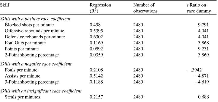
there was such a variable, it would be reported in the newspapers and data collection services. The absence of such a reporting boosts our confidence that there is not some important missing variable. However, to investigate this question more carefully, we regressed each individual player skill on his age, his height, his weight, each of these squared, and a 0,1 race dummy. The race dummy is significant in most cases, but not in the same way in each case. Table 6 reports the player skills and the t ratio on the race dummy variable.
Table 6
Blocked shots per minute 0.498 2480 9.791
Offensive rebounds per minute 0.5395 2480 4.041
Defensive rebounds per minute 0.6302 2480 4.041
Foul Outs per minute 0.1169 2480 3.868
Points per minute 0.0592 2480 9.231
2-Point shooting percentage 0.0359 2480 3.869
Skills with a negative race coefficient
Fouls per minute 0.2108 2480 −.3942
Assists per minute 0.5142 2480 −4.871
3-Point shooting percentage 0.1188 2480 −4.619
Skills with an insignificant race coefficient
Steals per minutes 0.2157 2480 0.686
aIn each case, we regressed the player skill on age, height, weight, and the square of each. We excluded all
players with<100 min played per season. The race dummy takes the value 1 if the player is black.
We explored alternative specifications to determine whether the playing time relation was robust. For instance, we included the team white/black player ratio as a control variable. We included a variable denoting whether a player was traded during the season. We deleted points scored per minute played from the regression. We reduced the sample to players who played at least 500 min during a season. We also estimated the playing time equation using only those individuals who played in at least 50 games. In all cases, the coefficient on race remains significant.
We divided teams into three classifications based on the team’s overall racial composition. The classifications are the middle half and the upper and lower quartiles of team racial composition.22 Then we reestimated the playing-time equation allowing for different race dummy variables in these three groups. The coefficients on the race dummy are reported in Table 7, and they are all positive. The class is significant, and in pairwise tests of equality the coefficient in the blackest quartile is different from the coefficients in the other two groups at the 10 percent level of significance. There is no evidence that the coefficient in the mixed half is different from the coefficient in the whitest quartile.
In addition, we allowed for different values of the race dummy variable in the minutes played equation depending on the racial composition of the underlying community (see Table 3). The results on the race dummies for this specification are reported in Table 8. We observe a positive and significant relation between playing time and race in the three SMSA race classifications. The overall class is significant, but the individual coefficients are statistically the same. Overall, the evidence suggests that black players play more than comparable white players in all cities and on all teams.
22In our sample the top quartile of teams with the largest portion of white players has a player ratio equal to or
Table 7
Coefficients on the race dummy in the playing time equation by different team racial classificationsa
Sample size: 2481; F ratio: 201.38; R2: 0.663
Team racial composition Parameter estimate t Ratio Prob>|t|
Blackest quartile 1.44 4.32 0.0001
Mixed half 1.64 5.54 0.0001
Whitest quartile 0.94 2.48 0.0134
aTeam racial composition is the ratio of total white players on the team to total number of black players on
the team for the year in question. The blackest quartile of teams has a white to black ratio of players of 0.2 or less. The whitest quartile has a white to black player ratio of 0.5 or greater. The mixed middle captures the remaining half of the teams. The F statistic on the class is 5.14 which is significant at the 1 percent level.
Table 8
Coefficients on the race dummy in the playing time equation across different SMSAsa Sample size: 2481; F ratio: 200.89; R2: 0.663
SMSA Parameter estimate t Ratio Prob>|t|
Blackest quartile 1.54 4.27 0.0001
Mixed half 1.49 5.14 0.0001
White quartile 1.31 1.31 0.0005
aSee Table 3 for a description of the SMSA variable. The F ratio on the SMSA class variable is 9.85 which is
significant at the 1 percent level. None of the pairwise tests of equality is significant.
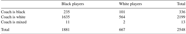
In the attendance results (Table 2), we find no significant relation between the race of the coach and attendance. We interpret this as additional evidence that fans are color blind. To explore the race issue further in the context of coaches, we investigated whether there was an impact on playing time which is related to the race of the player and the coach. We created a match variable which is one if the race of the coach and the player match and zero otherwise. In our player sample, 13.2 percent of the players had coaches that were black, and the rest had coaches that were white. Of the players, 73.8 were black. Table 9 reports the breakdown by race of player and coach.
Theχ2statistic of independence is 3.723 which is not significant at the 10 percent level. A black player is as likely to have a black coach as is a white player, and vice-versa. In total, we have 799 occasions where the race of the coach and the race of the player match,
Table 9
Frequency distribution of player race by race of coacha
Black players White players Total
Coach is black 235 101 336
Coach is white 1635 564 2199
Coach is mixed 11 2 13
Total 1881 667 2548
aThere is one case where there was a coaching change during the season, and one of the coaches was white
discarding the mixed situation. We estimated the playing time equation to determine if there was a propensity for white coaches to favor white players or black coaches to favor black players by including a dummy for the race match variable. In this specification, a player actually plays less, if he is the same race as his coach, but this result is not significant (the t ratio is−1.193 and the coefficient is small, less than half-a-minute per game). This result could be driven by the large portion of black players who play for white coaches. Consequently we estimated this effect separately for black and white coaches. The basic result persists that black players play more, but there is no significant difference between coaches in this regard. Both black and white coaches play black players more, other things the same.
6. A model of wage determination with racial discrimination by customers
Existing models of customer discrimination routinely employ an asymmetric approach. Some members of a majority group do not like members of a minority group. Here, we develop a more complete model where both groups in the model are biased. Suppose that there is customer-driven racial discrimination in professional basketball. That is, some white fans prefer to watch white players, and some black fans prefer to watch black players, other things the same. The remaining white and black fans are color blind. Furthermore, assume that discrimination declines by both whites and blacks as the number of preferred players is hired by a team. That is, the whites who care about race care less at the margin when the team is predominately white, and similarly for black fans. In this world, the actual impact of discrimination on hiring depends on the relative portions of black and white fans, assuming that income, preferences (specifically, discriminatory preferences), and other factors are constant across the two groups.
Consider a white fan attendance function
Aw=f (G, W, Pw) (1)
where the number of white fans who attend (Aw), the function of quality of play (games won) (G), the number of white players on the team (W), and the number of potential white fans in the area (Pw). Similarly, the black fan attendance function is
Ab=f (G, B, Pb) (2)
where Pbrepresents the black population in the community. We assume that white atten-dance increases with the number of white players, but at a decreasing rate.23 That is, ∂Aw/∂W >0 and∂2Aw/∂W2<0. And similarly for blacks, attendance increases as the number of black players increase, but at a decreasing rate.
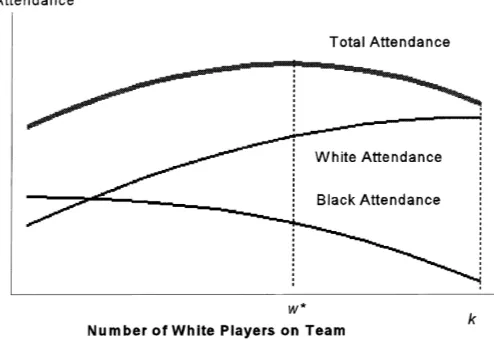
Both attendance equations are positive functions of the respective populations in Fig. 1. As the white (or black) population in the area increases, the relevant attendance function shifts up. The original white attendance function is drawn with population equal to P. When
23We employ a continuous characterization of the model under the presumption that a team can alter the number
Fig. 1. Attendance, racial composition, and population.
the white population in the relevant market increases to P′, the attendance function shifts up.
The NBA restricts roster size by fiat. The number of blacks on the team, B, plus the number of whites, W, sums to a constant, k. Total attendance, At, is the sum of white and black attendance,At =Aw+Ab. The derivative of total attendance with respect to white players on the team is:∂At/∂W = ∂Aw(·)/∂W −∂Ab(·)/∂B. Naturally, attendance is maximized when the slopes of the two attendance functions are equal (see Fig. 2). This point obviously depends on the relative proportions of whites and blacks in the community
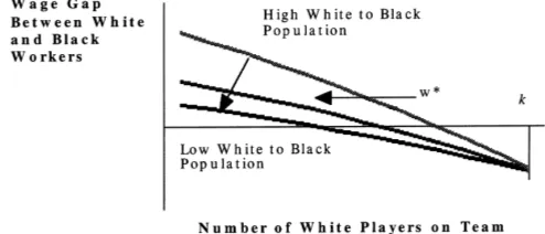
Fig. 3. Wage gap between black and white players.
and their respective attitudes toward each other. The optimal racial composition of the team is a function of the racial composition of the community.24
Consider Fig. 2. In general, the derived demand for black and white players of comparable skills will not be the same. Suppose the team is all black. Switching a white player for any black player induces an increase in white attendance that is not completely offset by a loss of black customers. The value of the marginal product of white players is greater up to the point where w∗of them are hired. After that point, the increase in white attendance from switching a white player for a black player reduces total attendance as the increase in white attendance is dominated by the loss of black fans.
Now consider Fig. 3. Here, we have drawn the wage gap as the racial composition changes from an all-black team to an all-white team. The hypothetical gap between the wage paid to a white player of certain skills lies above the wage that the firm would be willing to pay to a black player of similar skills, but that gap decreases as the white/black population ratio decreases towards one. As the ratio of white-biased fans increases relative to the number of black-biased fans, w∗(and the point of no wage gap) moves to the right.25 The critical point is that the wage gap vanishes at the attendance maximizing number of white players, w∗. When there are both black and white fans who are racially biased, the profit-maximizing team erases the gap between races by adjusting the proportions of white and black players. Accordingly, while we believe that racial prejudice can affect team composition, so long as the team is neither all white or all black, there can be no wage differential at the margin between players of equal abilities based on skin color. On these grounds, we are inclined to reject the racial discrimination explanation for any wage differentials between black and white players. Put another way, when the team has attained the correct racial composition, the owner is indifferent about the skin color of two players of similar abilities.26
24Of course, it is revenues and not attendance that matter, but absent a ticket price discrimination scheme across
races, revenues are a monotone function of attendance.
25There is no theoretical reason that w∗must lie to the left of k, and hence we cannot conceptually argue that we should observe no wage gap based on racial discrimination.
26Our model should not be interpreted to mean that fans only care about player skin color. Of course, they also
7. Odds and ends
In 1985–1986 the NBA instituted a salary cap. This restriction limits the total wage bill that a team can pay to its players. The limit has varied slightly from team to team based on a number of factors, but it was approximately US$ 53 million per year until the most recent (1999) CBA. We reestimated the minutes played equation (Table 5) allowing for different race coefficients in the two periods, the years without a salary cap (1980–1985) and the subsequent period.
First, the marginal minutes played per game for all players is lower after the salary cap. Since the total minutes played by the team is constant in the two periods, this suggests that one important impact of the salary cap is that each player plays less. In turn, this suggests that there is more turnover and more players playing with a salary cap than without. This conjecture is verified by the t test of the number of players on the team in the two periods. In the no salary cap period, the average number of players on a team was 13.48. After the institution of the cap, the average number of players on a team during a season increased to 14.2. The difference between these two averages is significant at the 1 percent level.27
The change in minutes played associated with the introduction of the salary cap was not race-neutral. In the minutes-played equation, the coefficient on black playing time is now 0.673 more minutes played per game than whites in the salary cap period. However, in the earlier period with no pay restriction, the difference is 0.974. Both coefficients are statistically significant from zero. The salary cap is associated with a smaller black-white playing time differential. Blacks play more than whites, and the salary cap reduced this difference, but not in a statistically significant way.
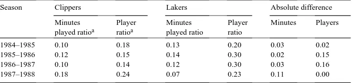
Lindsay and Maloney (1988) have advanced a sorting hypothesis about gender discrim-ination. They argue that if workers are gender biased, that is, men do not like to work with women and/or vice versa, and markets are thick, firms should sort plants and work facilities on gender basis to avoid the costs of having to pay men to work with women and vice-versa. Following this argument, if basketball fans are racially biased, then in large markets, where there are multiple NBA teams, the owners should separate the audience and specialize in one type team. For instance, there are two NBA teams in the New York City area, the Knicks and the Nets. If New York area fans are racially biased, both teams can benefit if one caters to white fans and the other to black fans. So if fans are biased, we ought to observe differences in the racial composition of teams in the same market. Besides New York, only Los Angeles has two NBA teams, the Lakers and the Clippers (since 1984–85).
In Table 10, the average absolute differences in minutes played and players in New York are 0.21 and 0.15, respectively. Both of these are significant at the 5 percent level. The New York market is sorted over this period. Table 11 repeats this exercise for Los Angeles. The means of the absolute differences in minutes and players are 0.21 and 0.08. The former is significant at the 10 percent level while the latter is not. Overall, combining the data
27With the salary cap, average salaries have still increased faster then the wage rate of entry-level jobs, and given
Table 10
Racial composition of NBA teams in New York
Season Knicks Nets Absolute difference
1980–1981 0.0 0.0 0.73 0.40 0.73 0.40
1981–1982 0.11 0.17 0.19 0.27 0.08 0.11
1982–1983 0.21 0.20 0.12 0.17 0.09 0.03
1983–1984 0.08 0.20 0.17 0.20 0.09 0
1984–1985 0.19 0.30 0.39 0.40 0.20 0.2
1985–1986 0.23 0.14 0.27 0.33 0.04 0.03
1986–1987 0.07 0.24 0.31 0.45 0.23 0.31
1987–1988 0.09 0.24 0.29 0.33 0.19 0.10
aRatio of total minutes played by whites to total minutes played by blacks and the ratio of the number of white
players to the number of black players over the whole season.
Table 11
Racial composition of NBA teams in Los Angeles
Season Clippers Lakers Absolute difference
1984–1985 0.10 0.18 0.13 0.20 0.03 0.02
1985–1986 0.12 0.15 0.14 0.30 0.02 0.15
1986–1987 0.10 0.14 0.12 0.30 0.03 0.16
1987–1988 0.18 0.24 0.07 0.23 0.11 0.00
aRatio of total minutes played by whites to total minutes played by blacks and the ratio of the number of white
players to the number of black players over the whole season.
from both cities, the means are 0.15 and 0.13, respectively, and both are significant at the 5 percent level.
Perhaps the best interpretation of these results is that New York is sorted and Los Angeles is not. There is, nonetheless, some evidence to suggest racial preferences by fans in large markets where the sorting hypothesis is most relevant.
8. Concluding remarks
The following combination of results seems to hold sway-in general, fans do not seem to care about race, owners pay black players less, and blacks play more. While there is some evidence of racial preferences by some fans, the weight of the evidence points toward a simple case of market segmentation price discrimination. Black players and potential black players have a more unresponsive labor supply with respect to providing services in this labor market than do white players.
players have more inelastic supply elasticities. It is quite plausible to suggest that because of discrimination and lower socio-economic standards, black children do not face the same opportunity sets as white children. The opportunity cost to a white youngster of playing or practicing basketball might be playing video games or vacationing in Europe with her parents, and so on, endlessly. The opportunity cost to a black youngster will be different (a truism), such that they practice more basketball, a sport requiring little physical capital except a public playground and a few friends. Black children may be more narrowly focused when young, and therefore, less responsive to wages in any market where they ultimately appear to be proficient workers. The end result of such a process is that the best black and white basketball players may have different opportunity costs and hence different elasticities of supply in the basketball labor market.28 This argument suggests that white players simply have more interesting and lucrative opportunities in the non-basketball world than do black players. This makes black players relatively unresponsive to wages in the basketball market. This is, of course, a story, designed to illustrate the complexity of explaining the price discrimination result. It is a constraint-driven story, however, capable of being tested. For example, do white players from Europe and Eastern Europe and the former Soviet Union face a pay differential similar to black players? What are SAT scores and other preparatory indicators, and what is the graduation rate of black and white college basketball players (Maloney and McCormick, 1993)? When current salary data become available, we can investigate whether there is a white-black wage differential for free-agent veterans. The price discrimination argument says the wage differential will have vanished for these players to the extent that owners are now competing with each other for their talents.
Acknowledgements
Thanks go to Robert Clement, Kris Krauza, and Erick Moore for help in assembling the database. We also appreciate the comments of session participants at the 1994 meetings of the Western Economics Association and seminar participants at Clemson University and the University of Chicago. The comments of Raymond Brastow, Donald Gordon, and Michael Maloney were particularly helpful. The usual caveat applies.
References
Andersen, R., LaCroix, S.J., 1991. Customer racial discrimination in major league baseball. Economic Inquiry 29, 665–677.
Bodvarsson, O.B., Brastow, R.T., 1994. Salary discrimination in the NBA: do race of management and the 1988 collective bargaining agreement matter? St. Cloud State and Longwood College, unpublished manuscript. Brown, R., Jewell, T., 1995. Race, revenues, and college basketball. Review of Black Political Economy 23, 75–90.
28Basketball appears to be an avocation that requires years of preparation. While there are exceptions, truly rare is
Brown, E., Spiro, R., Keenan, D., 1991. Wage and nonwage discrimination in professional basketball: do fans affect it? American Journal of Economics and Sociology 50, 333–345.
Burdekin, R.C.K., Idson, T., 1991. Customer preferences, attendance and the racial structure of professional basketball teams. Applied Economics 23, 179–186.
Clement, R., McCormick, R., 1989. Coaching team production. Economic Inquiry 27, 287–304.
Dey, M., 1997. Racial differences in national basketball association players’ salaries: a new look. American Economist 41, 84–90.
Goff, B.L., Tollison, R.D. (Eds.), 1990. Sportometrics. Texas A&M University Press, College Station.
Hamilton, B.H., 1991. Racial discrimination and professional basketball salaries in the 1990s. Applied Economics 29, 287–296.
Kahn, L.M., 1991. Discrimination in professional sports: a survey of the literature. Industrial Labor Relations Review 44, 395–418.
Kahn, L.M., Sherer, P.D., 1988. Racial differences in professional basketball players’ compensation. Journal of Labor Economics 6, 40–61.
Koch, J.V., Vander Hill, C.W., 1988. Is there discrimination in the black man’s game? Social Science Quarterly, 83–94.
Lott, J., Roberts, R., 1991. A guide to the pitfalls of identifying price discrimination. Economic Inquiry 29, 14–23. Lindsay, C.M., Maloney, M.T., 1988. A model and some evidence concerning the influence of discrimination on
wages. Economic Inquiry 26, 635–658.
Maloney, M.T., McCormick, R.E., 1993. An examination of the role that intercollegiate athletic participation plays in academic achievement: athletes’ feats in the classroom. Journal of Human Resources 28, 555–570. Marburger, D.R., 1996. Racial discrimination in long-term contracts in major league baseball. Review of Black
Political Economy 25, 83–94.