A comparison of some inverse methods for estimating the
initial condition of the heat equation
Wagner Barbosa Muniza;∗, Haroldo F. de Campos Velhob, Fernando Manuel Ramosb
a
Instituto de Matematica, Universidade Federal do Rio Grande do Sul, Porto Alegre, RS, Brazil
bLaboratorio Associado de Computac˜ao e Matematica Aplicada, Instituto Nacional de Pesquisas Espaciais, CP 515,
12201-970 S˜ao Jose dos Campos, SP, Brazil
Received 29 October 1997; received in revised form 23 December 1997
Abstract
In this work we analyze two explicit methods for the solution of an inverse heat conduction problem and we confront them with the least-squares method, using for the solution of the associated direct problem a classical nite dierence method and a method based on an integral formulation. Finally, the Tikhonov regularization connected to the least-squares criterion is examined. We show that the explicit approaches to this inverse heat conduction problem will present disastrous results unless some kind of regularization is used. c1999 Elsevier Science B.V. All rights reserved.
Keywords:Inverse problems; Least-squares method; Spectral formulation; Tikhonov regularization
1. Introduction
Inverse problems have certainly been one of the fastest growing areas in various application elds. Science and industry are both responsible for this growth in the last years. The main diculty in the treatment of inverse problems is the instability of their solution in the presence of noise in the observed (measured) data, that is, the ill-posed nature of the problem in the sense of Hadamard. This problem not only dees easy solution, but has served to discourage the type of massive study that has accompanied direct or well-posed problems [10, 13]. One could generically classify inverse problems into three types (all of them based on observations of the evolution of the involved physical system): identication of physical parameters orparameter identication; determination of the initial state of the system and; determination of the boundary conditions [3].
We will deal here with the second type of inverse problems in the eld of heat transfer, that is, the determination of the initial condition from transient temperature measurements taken within the nite medium at a time t= ¿0 — the backwards heat equation [5, 7, 11].
∗Corresponding author. E-mail: [email protected].
One could say that inversion techniques may be generically divided into two categories:
• Explicit: Inversion methods which are obtained through an explicit inversion scheme involving the operator representing the direct problem.
• Implicit: Which present an iterative character that exhaustively explores the model space (solution space) until a stopping criterion is satised, considering, of course, the available data.
In this article we will examine some inversion techniques in order to estimate the initial tem-perature distribution of an inverse heat conduction problem (IHCP), from which two of them are classied as explicit inversion techniques and the other one is implicit.
2. The direct problem
The direct (forward) problem consists of a transient heat conduction problem in a slab with adiabatic boundary condition and initially at a temperature denoted by f(x).
The mathematical formulation of this problem is given by the following heat equation:
@2T(x; t)
where T(x; t) (temperature), f(x) (initial condition), x (spatial variable) and t (time variable) are dimensionless quantities and = [0;1].
The solution of the direct problem for a given initial condition f(x) is explicitly obtained using separation of variables [2], for (x; t)∈×R+: represents the integral normalization (or the norm).
The above representation requires that the initial temperaturef(x) be a bounded function satisfying Dirichlet’s conditions in the interval [2].
One must observe that the norm, N(m), is dened as
In particular, with the adiabatic boundary conditions, the eigenvalues and eigenfunctions for the problem dened by Eq. (1) can be expressed, respectively, as
m=m;
3. The inverse problem
As explained previously, a transient heat conduction problem in a slab is considered, where both boundaries are kept insulated. Here the inverse problem consists of the determination of the initial temperature distribution f, since the temperature distribution T is given for the time t= ¿0. In order to dene the discrete version of the problem we consider that the transient temperature T is available at a nite number of dierent locations on the medium. In actual problems, this temperature is usually found empirically and hence known only approximately. This problem is a genuinely ill-posed problem in the sense of Hadamard, as we will see below.
The present inverse problem admits an analytical solution obtained from Eq. (2), using the or-thogonality property of the eigenfunctions X(m; x):
Z
X(m; x)X(k; x) dx=mkN(k);
where mk is the Kronecker’s delta. Therefore we have:
Theorem 1. If the temperature T(x; t)is known for the time t= ¿0 on the whole spatial domain
; then the initial temperature f(x) is given by
f(x) =
Proof. ( ¿0): We express the solution of the direct problem as
T(x; ) =
Applying the initial condition (t= 0) and expression (5) we obtain
Using the result of Theorem 1, we can show the ill-posedness of the backwards heat equation, as follows:
Theorem 2. If we consider the problem of determining the initial condition; where f; T∈L2();
then f does not depend continuously on the data T; that is; the problem is ill-posed in the sense of Hadamard; since the stability requirement is not satised.
Proof. Consider the initial conditionsf1; f2∈L2() such thatf2(x) =f1(x)+KX(n; x), withK∈R\ {0} andn∈N. Assume that the corresponding transient solutions (at a xed ¿0) are, respectively, the distributions T1(x; ); T2(x; ). By the linearity, see Eq. (2), we have
Thus, for any number K, the quantity kT2 −T1k2 can be made arbitrarily small by choosing n
suciently large. Similarly, if we measure the dierence between f1 and f2 in the L2-metric with
K6= 0, we obtain
Hence, with arbitrarily small discrepancies between T1 and T2, one can choose n and K in such
a way that the discrepancy between the corresponding solutions (f1 and f2) can be arbitrary.
kT1−T2k2→0 but kf1−f2k29 0:
One can easily note that, according to the proof of Theorem 2, we have
kf2−f1k2= e
2
nkT
2−T1k2;
which means that the error in the solution of this inverse problem is amplied exponentially by the factor e2
n. Clearly, the error becomes worse as increases, but even with a small ¿0
the exponential amplication of the error remains. In this context, a simple example arises if we suppose that the data measurement error = O(e−10) and we put 2
n= 20, then we obtain an error in the solution = O(e10).
4. Inversion techniques
We primarily present three approaches which would seem very natural (or appropriate) if we were dealing with a well-posed problem, for which the uniqueness, existence and stability are ensured. The rst two are classied as explicit, according to the initial explanation.
4.1. The linear explicit method
We consider Eq. (2), with a xed time ¿0, and we rewrite it as a Fredholm integral equation of the rst kind quadrature formula (e.g., Simpson’s rule, trapezoidal rule), reduce the integral equation (6) to a system of linear equations
T(xj; ) =X j
aijf(xi):
So we can directly invert this linear approximation, that is, we invert the projection, onto a nite-dimensional space, of the operator associated to the direct problem.
4.2. Discrete backward inversion — sequential technique
This so-called second explicit method is based on a backward-time centered-space discretization of the heat equation (BTCS), so that an explicit scheme is obtained such that f is a function of T.
Notation. T(xi; tn) =Tin, where tn=nt, xi=ix and t, x are, respectively, the temporal and
4.3. The implicit method: least squares
The least-squares approximation, in the sense of the minimum norm, can guarantee the existence and uniqueness, but this solution can be unstable in the presence of noise in the experimental data, requiring thus the use of some regularization technique [13]. The regularized solution is obtained by choosing the function f that minimizes the following functional:
M[ ˜T ; f] =kAf−T˜k2
2+ [f]; (7)
where ˜T= ˜T(x; ) is the experimental data (t= ¿0), A is an operator that maps the parameter set {f}into the results set {T}, [f] denotes the regularization term (Tikhonov), is the regularization parameter, and k · k2 is the 2-norm.
The regularization parameter is chosen numerically, through an a posteriori parameter choice rule, assuming that the statistics of the measurement errors is known. These numerical experiments are based on the Morozov’s discrepancy principle: ∗ is optimum when
Nx2∼ kAf∗−T˜k22=:R(f∗) ( =M ∗
[ ˜T ; f∗]−∗[f∗]);
where is the standard deviation of the measurement errors [1, 6].
4.3.1. Regularization functions
As already mentioned, it can be assumed that there is a unique solution, in the minimum norm least-squares sense, for a given inverse problem. According to Tikhonov [13], ill-posed problems can yield stable solution if sucient a priori information about the true solution is available. Such information is added to the least-squares approximation by means of a regularization term, in order to complete the solution of the inverse problem. Therefore, one can say that it is natural to expect that the regularization parameter is a good compromise between the data tting and the smoothing requirement. The regularization functions used in this paper are described below: they correspond to the so-called Tikhonov regularization.
4.3.2. Tikhonov regularization
The regularization technique presented by Tikhonov can be expressed by [13]
[f] =
where f(k) denotes the kth derivative relative to x, since f=f(x), and the regularization parameters
k¿0. The regularization eect for zeroth order is to reduce the oscillations on the parameter vector (smooth function f(x)). A rst-order regularization tends to make |df=dx| ≈0, that is, f(x) is approximately constant.
Clearly, as k→0 the least-squares term in the objective function is over-estimated, what might not give good results in the presence of noise. On the other hand, if k→ ∞, all consistency with the information about the system is lost.
Considering the zeroth order Tikhonov regularization, note that one can easily show that the functional M[ ˜T ; f], as dened in (7), is monotonically increasing with respect to and that f
5. Numerical realization of the direct problem
Since the implicit methods require iterative solutions, where numerical techniques are applied, a numerical solution to the direct problem (1) is necessary.
Here we will consider two dierent approximations to the problem:
1. A second-order (time and space) nite dierence method of discretization of the heat equation: Crank–Nicolson [12].
2. An integral approach, which is based on a linear approximation of the function f in the sub-domains of the whole spatial domain, such that a semi-analytical approximation is established. In this case, the approximation will be outlined below by considering Eq. (2):
The integral R
f(x)X(m; x
′
) dx′
in Eq. (2) is approximated as follows: the interval is splitted into Nx sub-intervals i= (xi; xi+1), such that xi+1=xi+i at i= 0; : : : ; Nx, where i is a positive able. Therefore, the integral in is given by
Z
Substituting Eq. (9) into Eq. (2) yields
T(x; ) =
In this article we have described three models in order to solve the backwards heat equation and we now give an example in order to illustrate the accuracy of the methods.
The numerical experimentation of the proposed inversion methods (Section 4) is based on a triangular test function
f(x) =
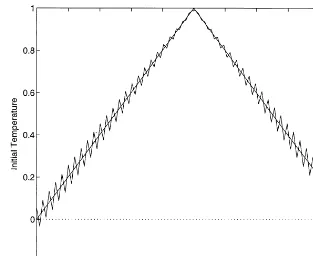
Fig. 1. Explicit inversion:= 10−4
without noise.
The experimental data (measured temperatures at a time ¿0), which intrinsically contains errors, is obtained by adding a random perturbation to the exact solution of the direct problem, such that
Texperimental=Texact+U;
where is the standard deviation of the errors and U is a random variable taken from a uniform distribution (U∈[−1;1]).
It is important to observe that the spatial grid consists of 100 points (Nx= 100) and the so-called inversion method was developed through the trapezoidal rule.
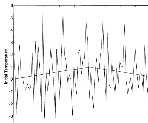
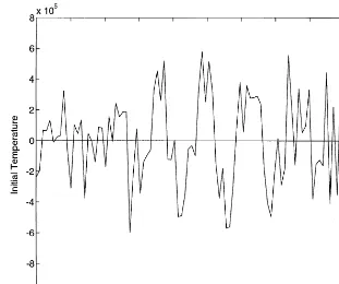
One can easily conclude that the explicit inversion method, developed in Section 4.1, which is based on a quadrature formula (trapezoidal rule), does not give satisfactory results, since Figs. 1–4 show that numerical solutions using this methodology present disastrous oscillations, even without noise in the data (Figs. 1 and 2). Note that the magnitude of the numerical solution, when = 0:008 and = 0:05, is O(105)! A very undesirable result.
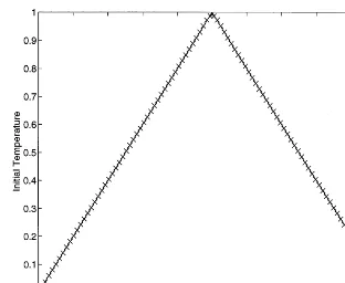
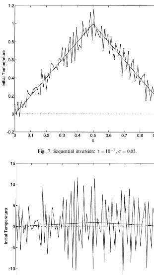
However, it is observed (Figs. 5–8) that the agreement of the numerical solution as obtained by the sequential scheme of inversion (Section 4.2) with the exact solution is ‘good’ only when there is no noise (= 0). This approach also presents a numerical solution with strong oscillatory characteristics in the presence of measurement error in the data = 0:05.
Fig. 2. Explicit inversion:= 0:008 without noise.
Fig. 3. Explicit inversion:= 10−4
Fig. 4. Explicit inversion:= 0:008; = 0:05.
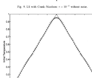
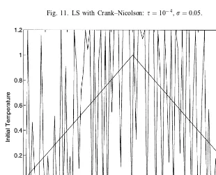
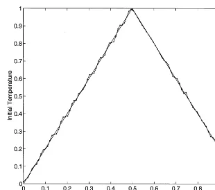
Now, note that the Figs. 9–16 present the numerical solutions obtained by two methods which solve the direct problem associated to Eq. (7): the Crank–Nicolson and the spectral method. It is observed that, under errorless data, both methods present a numerical solution very close to the triangular function. However, with noisy data, the spectral method presents the best results, which becomes clear if we compare Figs. 11 and 15. The advantage of the spectral approach is that the time dependence is exactly represented and only the spatial domain is approximated.
It is clear that the LS methodology associated to the spectral method presents better results than the so-called sequential and linear explicit inversion. Nevertheless, the LS methodology or residual minimization does not eliminate the instability of the solution under the presence of noise, see Fig. 16. So, a regularization method will be required: we use a zeroth- and rst-order Tikhonov regularization with the Morozov’s discrepancy principle as the parameter choice rule.
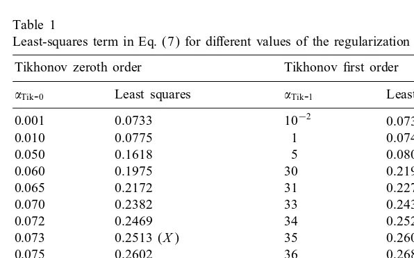
If we eectively want to apply some kind of regularization, as Tikhonov, which means ¿0, then the discrepancy principle implies that a suitable regularized solution can be obtained. Since the spatial resolution is Nx= 100, the optimum is reached for R(f∗)≈ nX2= 0:25. Table 1 shows the least-squares term R(f∗) obtained for dierent values of , and the optimum value is pointed out (X) for each regularization method.
Fig. 5. Sequential inversion:= 10−4
without noise.
Fig. 7. Sequential inversion: = 10−4
; = 0:05.
Fig. 9. LS with Crank–Nicolson: = 10−4 without noise.
Fig. 11. LS with Crank–Nicolson:= 10−4
; = 0:05.
Fig. 13. LS with spectral method:= 10−4
without noise.
Fig. 15. LS with spectral method:= 10−4
; = 0:05.
Fig. 17. Inversion by Tikhonov-0 (with spectral method), = 0:008; = 0:05 and where (–) exact solution; (· · ·)= 10; (· ·) = 10−4; (·+·) = 0:073.
Table 1
Least-squares term in Eq. (7) for dierent values of the regularization parameter Tikhonov zeroth order Tikhonov rst order
Tik-0 Least squares Tik-1 Least squares
0.001 0.0733 10−2 0.0732
0.010 0.0775 1 0.0740
0.050 0.1618 5 0.0800
0.060 0.1975 30 0.2196
0.065 0.2172 31 0.2275
0.070 0.2382 33 0.2437
0.072 0.2469 34 0.2520 (X)
0.073 0.2513 (X) 35 0.2600
0.075 0.2602 36 0.2687
0.077 0.2694 37 0.2773
0.080 0.2824 38 0.2859
0.090 0.3330 39 0.2946
0.100 0.3864 40 0.3033
Fig. 18. Inversion by Tikhonov-1 (with spectral method),= 0:008; = 0:05 and where (–) exact solution; (· · ·)= 1000; (· ·) = 10−2; (××) = 34.
7. Final comments
The preliminary approaches to the solution of this inverse problem evidence its genuine ill-posedness. When we treat an ill-posed (or inverse problem), we cannot apply a methodology which would seem natural if we were dealing with a well-posed (or direct problem). We have to evaluate all available information about the physical system.
The direct problem seems to be best solved if the spectral methodology is employed: the advantage of this formulation consists of its semi-analytical nature.
The implicit strategy and regularization techniques adopted in this paper yield good results in reconstructing the initial condition. The discrepancy criterion was ecient to estimate the Lagrange multiplier in the analyzed cases, and it was successfully used for other initial conditions. The chosen regularization techniques — zeroth- and rst-order Tikhonov regularization — are suitable for solving the proposed inverse problem.
Acknowledgements
References
[1] B. Blackwell, J.V. Beck, C.D. St. Clair, Inverse Heat Conduction, Wiley, New York, 1985.
[2] H.S. Carslaw, J.C. Jaeger, Conduction of Heat in Solids, Oxford at the Clarendon Press, London, 1959.
[3] H.W. Engl, M. Hanke, A. Neubauer, Regularization of Inverse Problems, Kluwer Academic Publishers, Dordrecht, 1996.
[4] E04UCF, NAG Fortran Library Mark 13, Oxford, UK, 1993.
[5] H. Han, D.B. Ingham, Y. Yuan, The boundary element method for the solution of the backward heat conduction equation, J. Comput. Phys. 116 (1995) 292–299.
[6] V.A. Morozov, Regularization Methods for Ill-Posed Problems, Michael Stessin, New York, 1993.
[7] W.B. Muniz, F.M. Ramos, H.F. Campos Velho, Regularized solutions of an inverse heat conduction problem: initial condition estimation, Proc. XVIII CILAMCE — Iberian Latin–American Conf. on Computational Methods in Engineering, vol. I, Braslia, Brazil, 1997, pp. 517– 524.
[8] F.M. Ramos, H.F. Campos Velho, Reconstruction of geoelectric conductivity distributions using a rst-order minimum entropy technique, Proc. 2nd Internat. Conf. on Inverse Problems in Engineering: Theory and Practice, vol. 2, Le Croisic, France, 1996, pp. 195 –206.
[9] F.M. Ramos, A. Giovannini, Resolution d’un problem inverse multi-dimensional de diusion de la chaleur par la methode des elements analytiques et par le principe de l’entropie maximale, Internat. J. Heat Mass Transfer 38 (1995) 101–111.
[10] P. Sabatier, Inverse problems — an introduction, Inverse Problems 1 (1985) 1– 4.
[11] A.J. Silva Neto, M.N. Ozisik, An inverse heat conduction problem of estimating initial condition, Proc. 12th Brazilian Congress of Mechanical Engineering, Braslia, Brazil, 1993.
[12] G.D. Smith, Numerical Solution of Partial Dierential Equations: Finite Dierence Methods, Oxford University Press, New York, 1985.