ANALYSIS
A test of policy labels in environmental choice modelling
studies
R.K. Blamey
a,*, J.W. Bennett
b, J.J. Louviere
c, M.D. Morrison
d, J. Rolfe
e aUrban and En6ironmental Program,Research School of Social Sciences,Australian National Uni6ersity,ACT0200,AustraliabEconomics and Management,Uni
6ersity of NSW,Canberra,ACT,Australia cDepartment of Marketing,Sydney Uni6ersity,Sydney,NSW,Australia
dCharles Sturt Uni6ersity,Bathurst,NSW,Australia eCentral Queensland Uni6ersity,Emerald,Qld,Australia
Received 22 February 1999; received in revised form 27 July 1999; accepted 28 July 1999
Abstract
A question that arises in the application of environmental choice modelling (CM) studies is whether to present the choice sets in a generic or labelled form. The former involves labelling the policy options to be presented to respondents in a generic way, for example, as ‘option A’, ‘option B’, etc. The labelled approach assigns alternative-specific descriptors to each option. These may relate to the names of proposed policies, different locations or any other policy-relevant details. Both approaches have their advantages. A potential advantage of using alternative-spe-cific labels is that respondents may be better able to base their choices on the true policy context. This can increase predictive validity whilst at the same time reducing the cognitive burden of the CM exercise. A potential advantage of the generic labelling approach is that respondents may be less inclined to base their choices wholly or largely on the labels, and as a consequence, may provide better information regarding trade-offs among attributes. The two approaches to choice set design are compared in the context of a CM study of the values of remnant vegetation in the Desert Uplands of Central Queensland. Results indicate a difference in the cognitive processes generated by choice models using the different approaches. This difference is reflected in both the alternative-specific constants and the taste parameters, and cannot be accounted for by differences in error variance across the two treatments. The implications for environmental valuation are discussed. © 2000 Elsevier Science B.V. All rights reserved.
Keywords:Choice modelling; Stated preferences; Non-market valuation
www.elsevier.com/locate/ecolecon
1. Introduction
Recent years have seen increasing interest in the use of conjoint-based stated preference methods for the assessment of environmental values. Al-though the contingent valuation method (CVM) remains the most commonly applied stated prefer-* Corresponding author. Fax: +61-2-62490312.
E-mail address: [email protected] (R.K. Blamey)
ence technique in this area, techniques such as choice modelling (CM), also referred to as the choice experiment, are increasingly being favoured.
Whilst applications of the discrete choice CVM require respondents to choose between a base option and a single alternative, respondents to CM exercises are typically presented with six to ten choice sets, each containing a base option and two or three alternatives. They are required to indicate which option they prefer in each choice set. The levels of the attributes characterising the different choice set options are varied according to an experimental design, permitting estimates of the relative importance of the attributes describ-ing the options to be obtained. Rather ‘than bedescrib-ing questioned about a single event in detail, as in CVM analysis, subjects are questioned about a sample of events drawn from the universe of possible events of that type’ (Boxall et al., 1996, p. 244).
A fundamental question that arises in the appli-cation of CM is whether to present the choice sets in a generic or labelled form. The generic form involves assigning generic labels to each alterna-tive in the choice set, such as ‘alternaalterna-tive A’, ‘alternative B’ etc. The labelled form involves assigning labels that communicate, directly or in-directly, information regarding the tangible and/
or intangible qualities of the alternatives. In marketing applications, labels tend to consist of brand names and logos, which consumers have learnt to associate with different product charac-teristics and feelings. In the context of environ-mental policy, labels tend to refer to sites, locations, policy names or other descriptors.
An advantage of assigning issue-relevant and alternative-specific labels is that responses will better reflect the emotional context in which pref-erences are ultimately revealed. For example, a respondent may have a predisposition toward vis-iting a particular recreation site because he or she has fond memories from a past visit. This factor may not be reflected in the results of a CM exercise that describes sites purely in terms of tangible attributes involving recreation opportuni-ties, camping faciliopportuni-ties, proximity and cost. Often,
the most plausible way of including such informa-tion is in the form of a label. This informainforma-tion not only increases predictive validity, but may also make the exercise less cognitively demanding.
Offsetting this potential advantage of labelled choice set configurations is the likelihood that generic configurations may encourage more dis-cerning and discriminating responses. Instead of respondents being able to base their responses wholly or largely on the alternative with the most superficially attractive label or descriptor, respon-dents are required to consider differences in policy options as described by the attributes listed in the choice sets (Blamey et al., 1997; Morrison et al., 1997). The resultant more informed and deliber-ated preferences may be desirable from a non-market valuation perspective (Mitchell and Carson, 1989).
In this paper, the effects of employing labelled rather than generic choice-set configurations are considered. A split sample approach is used. Two statistically equivalent samples of the Brisbane population were presented with the same basic CM questionnaire, with the exception that one employed a generic approach and the other a labelled approach. This enables a direct compari-son of the two sets of results with a view to assessing the degree of convergent validity. These issues are considered in the context of a CM study of remnant vegetation values in the Desert Up-lands of Central Queensland, Australia.
The paper is structured as follows. The theoret-ical basis of CM is briefly reviewed in Sections 2 and 3, and the case study is introduced in Section 4. Methods are then presented in Sections 5 – 7, and the results are presented in Section 8. Some conclusions are finally drawn.
2. Theoretical basis of choice modelling
Choice modelling has its origin in conjoint analysis, information integration theory in psy-chology and discrete choice theory in economics/
one or more alternatives into the utility associated with the individual attributes of those alternatives (Louviere, 1988). As such, these approaches have foundations in Lancaster’s (1966, 1991) modern consumer theory.1
Environmental applications of CM include Adamowicz et al. (1994), Boxall et al. (1996), Rolfe and Bennett (1996), Adamowicz et al. (1998), Hanley et al. (1998a,b), Morrison et al. (1999) and Blamey et al. (1999). Boxall et al. (1996) observe that CM is attractive for environ-mental valuation because it relies on the same model structures as referendum CVM models and discrete choice travel cost models (p. 244 – 5).
Both CM and the dichotomous-choice CVM have their theoretical bases in random utility the-ory (RUT). According to RUT, the ith respon-dent is assumed to obtain utility Uij from thejth alternative in choice set C. Uij is held to be a function of both the attributes of the alternatives (Xjkrepresenting thekth attribute value of thejth alternative) and characteristics of the individual, Si. Uij is assumed to comprise a systematic com-ponentVijand a random componenteij. WhilstVij relates to the measurable component of utility,eij captures the effect of omitted or unobserved vari-ables. We thus have
Uij=Vij(Xij, Si)+eij (1)
Respondent i will choose alternative h in prefer-ence to j if Uih\Uij. Hence, the probability of i choosingh is:
Pih=Prob(Uih\Uij) for allj in C,j"h
=Prob(Vih−Vij\eij−eih), for allj in C, j
"h (2)
The eij for all j in C are typically assumed to be independently and identically distributed (IID) and in accordance with the extreme value (Gum-bell) distribution. This gives rise to the multino-mial logit model, commonly employed in discrete
choice modelling, of which the binary logit used in CVM studies is a special case:
Pih=
exp[lVih]
%
jC
exp[lVij]
(3)
where l is a scale parameter, which is inversely proportional to the variance of the error term, and commonly normalised to 1 for any one data set (Ben-Akiva and Lerman, 1985). An estimated linear-in-parameters utility function for the jth alternative often takes the following form:
Vj=ASCj+b1X1+b2X2+b3X3+…bkXk
+…bnXn+g1(S1ASCj)+…
+gm(SmASCj) (4)
where there are n attributes with generic coeffi-cients across alternatives, and m individual-spe-cific variables multiplied by an alternative-specific-constant (ASC). The ASCs capture the mean effect of the unobserved factors in the error terms for each alternative. This provides a zero mean for the error terms and causes the average probability of selecting each alternative over the sample to equal the proportion of respondents actually choosing the alternative. Socioeconomic and attitudinal variables can be included by inter-acting them with the alternative-specific constants (as shown in Eq. (4)) and/or the attributes (not shown). ASCs should be included regardless of whether generic or alternative-specific labels are employed. The inclusion of alternative-specific la-bels simply alters the interpretation of the esti-mated ASCs.
The inclusion of ASCs helps mitigate inaccura-cies due to violations in the assumption of inde-pendence of irrelevant alternatives (IIA) (Train, 1986). This assumption, which arises from the above-mentioned IID assumption, implies that the ratio of the choice probabilities for any two alternatives be unaffected by the addition or re-moval of alternatives. This is equivalent to assum-ing that the random error components of utility are uncorrelated between choices and have the same variance (Carson et al., 1994). Violations of the IIA assumption render the MNL model inappropriate.
One way of circumventing the IIA property is to allow for correlations among the error terms within different subsets or classes of alternatives by estimating a nested logit model (McFadden, 1978; Daganzo and Kusnic, 1993). In a two-level nested logit model, the probability of an individ-ual choosing thehth alternative in therth branch (Phr) is represented as:
Phr=P(h/r)P(r) (5)
where P(h/r) is the probability of an individual choosing thehth alternative conditional on choos-ing the rth class of outcome, located in the rth branch of the tree.P(r) is the probability that the individual chooses the rth branch. Following Kling and Thomson (1996):
P(h/r)=exp[Vhr/ar]
is referred to as the inclusive value. This is a measure of the expected maximum utility from the alternatives associated with the rth class of alternatives. Hr is the number of alternatives in branchr, and Vhris the utility of the hth alterna-tive in the rth branch. The coefficient of the inclusive value, ar, measures substitutability across alternatives. When substitutability is greater within rather than between alternatives, 0BarB1. In this case, respondents will shift to other alternatives in the branch more readily than they will shift to other branches (Train et al., 1987). The popularity of the nested logit model is in part due to the way in which nested decision structures lend themselves to behavioural interpretations.
Welfare estimates are obtained in CM studies using the following general formula described by Hanemann (1984):
wheremis the marginal utility of income,Vi0and Vi1represent the indirect observable utility before and after the change under consideration, and C is the choice set. In CM, the absolute value of the coefficient of the monetary attribute in the choice model is taken as an estimate ofm. Changes inVi0 or Vi1can arise from changes in the attributes of alternatives or the removal (or addition) of alter-natives altogether. For example, in recreational site studies where alternatives are substitutes in consumption, the removal of an alternative from the choice set might correspond to a site closure, which one would expect to result in a welfare loss. When alternatives are substitutes in ‘production’, such as when a single solution has to be chosen from a set of feasible solutions, the removal of alternatives can be used to estimate selection probabilities and welfare implications based on different choice sets.
When the choice set includes a single before and after policy option, Eq. (9) reduces to:
W= −1
m[ln(e
Vi0)−ln(eVi1)]= −1
m[Vi0−Vi1] (10)
In the case of changes in a single attribute, this further reduces to −bj/m when a linear in parameters utility function is employed. This is equivalent to calculating the ratio of marginal utilities for the attribute in question and the mon-etary attribute, or the marginal rate of substitu-tion (MRS) (Hensher and Johnson, 1981). Kling and Thomson (1996), Herriges and Kling (1997), Choi and Moon (1997) consider the application of Eq. (9) in the nested logit case.
3. Labels and choice
brand names and other labels may exist that are imbued with specific emotional associations that are not obviously tied to specific product at-tributes. Such emotional associations are some-times referred to as ‘freestanding emotions’ (Rossiter and Percy, 1997, p. 123). They are dis-tinct from the weights that are associated with specific attributes.
In the terminology of Eq. (4), the variables X1−Xn reflect the product attribute values and the b1−bn reflect the weights of the attributes. Differences between perceived and objective product attribute values can be accounted for when substituting values into Eq. (4) to calculate market share and/or compensating surplus (Adamowicz et al., 1996).
The influence on choice of freestanding emo-tions is captured by the ASCs in Eq. (4), along with any other systematic unobserved effects. Dif-ferent labels may impose difDif-ferent demand arte-facts on the task in the form of inferences that cannot be observed, thereby producing differences in the ASCs. The ASCs may also capture the influence of any ‘presentation effects’. For exam-ple, the tendency of some respondents to favour middle alternatives in the choice set, on the basis that this represents some form of compromise between conflicting goals, would be reflected in the ASCs (Blamey et al., 1997; Morrison et al., 1997).
Although individuals are assumed above to sum the weighted benefit beliefs, and any freestanding emotions, to form an attitude and purchase inten-tion, they can, of course, employ any of a number of compensatory and non-compensatory choice rules. As observed by Simon (1955), they may seek to simplify their decisions by either restrict-ing the scope of the decision problem, for exam-ple, by limiting the number of attributes to be evaluated, or by simplifying the decision rule used to evaluate them. In the context of the present study, respondents may develop choice rules based around the demand artefacts contained within the labels but also reflecting certain limited attribute contingencies. For example, a respon-dent may decide to adopt a choice rule in which one labelled option is always preferred unless the level of a selected attribute exceeds a given
threshold. A labelled approach may make it easier for respondents to process the options, by reduc-ing the number of difficult attribute trade-offs requiring consideration. A consequence may be lower weights on the attribute parameters.
4. Research design and hypotheses
The main objective in this paper is to consider the effect of employing labelled rather than generic choice-set configurations. A split sample approach is used, with two statistically equivalent samples of the Brisbane population being pre-sented with the same basic CM questionnaire. The difference between the two questionnaire versions is that one presents alternatives in a generic form and the other in a labelled form. The labelled form involves the inclusion of policy labels as constant headers in the choice set alternatives, along with the use of alternative-specific attribute levels.
Two alternative ways of constructing the com-parison are apparent. The first involves including the policy names as labels for the alternatives in a labelled treatment, and as an attribute in a generic treatment. Only in the generic treatment would the policy names vary according to an experimen-tal design. This approach has the advantage of controlling for the amount and type of informa-tion conveyed to respondents: the only difference is the location of the information within the choice sets. The second approach is similar to the first, with the exception that the policy names are removed altogether in the generic treatment. Whilst this approach may introduce a degree of omitted variable bias, it has the potential advan-tage of producing more discerning responses, par-ticularly when labels have significant emotional and symbolic content. Respondents may focus more closely on what they are choosing, if they are unaware of the particular policy label with which a set of attributes are associated.2 More
informed trade-offs may be desirable for welfare estimation and environmental policy-making. An-other potential advantage of this second approach is that it may be less susceptible to problems associated with implausible combinations of pol-icy names and attribute levels.
Both approaches are subject to complications from a modelling perspective. With the first ap-proach, complications can arise if the policy at-tribute interacts with other atat-tributes. Obviously, the likelihood of such interactions depends in part on the information communicated by the policy names. For example, policy names that communi-cate information regarding percentages of vegeta-tion cleared may interact with other attributes pertaining to species lost. Estimating such interac-tions not only requires a special experimental design, but also complicates model comparisons since different specifications may be involved.
The second approach avoids the need to model attribute interactions, although models with alter-native-specific attribute parameters may need to be considered. However, these do not require special experimental designs. The main complica-tion that arises with this approach stems from the fact that the policy labels may impose a demand artefact on the task in the form of inferences about the alternatives that we cannot observe. Including the policy labels may simply shift re-spondents’ attention from the attributes to the labels. Unobservable interactions between the la-bels and the attributes may result in different parameter vectors. It is thus important to consider whether the overall welfare implications of given policy options remain constant across the two treatments.
The second approach to comparing labelled and generic choice set configurations is adopted in this study. The two treatments are compared in terms of attribute taste vectors, marginal rates of substitution, ASCs and compensating surpluses. The following hypotheses are tested:
4.1. Hypothesis 1
Differences in attribute taste parameters across data sets imply different cognitive processes. If respondents choose the option with the label most
closely aligning with their held values and atti-tudes, with little or no regard for the outcomes described by the attributes, one would expect significant differences between attribute parame-ters across treatments. It is also possible that some attribute parameters in the labelled model will not be statistically significant. The first hy-pothesis is:
H1: bL=bG=b
where the superscripts Land Gon the coefficient vectors refer to the labelled and generic treat-ments, respectively, corresponding to the data sets XL and
XG. Testing this hypothesis requires dif-ferences in the scale factor lbetween data sets to be taken into account. Following Swait and Lou-viere (1993), precise estimates of the relative scale factor can be obtained by stacking the two data sets, conducting a one-dimensional grid search over different values ofl, and performing a likeli-hood ratio test.3
Whilst the Swait – Louviere test can in principle be applied to the entire parameter vector, or any subset thereof, in practice the test is usually re-stricted to the terms not involving the ASC. In-cluding the ASC terms represents a stringent requirement, requiring not only that the response to the attributes be proportional across the two data sources, but also that the aggregate shares be equal (Swait et al., 1994). It can also be difficult to develop meaningful hypotheses and interpreta-tions regarding the ASC terms, as they relate to unobserved effects.
In the event that H1 is rejected for a given set of parameters, it is desirable to try and isolate the source of the violation. This can be done by postulating sources of the violation, for example, by examining the plot of coefficient vectors, and allowing these parameters to differ between data sets. H1 is then repeated for the component of the
parameter vectors subject to the equality restriction.
4.2. Hypothesis 2
The second hypothesis is targeted towards the detection of differences in the marginal rates of attribute substitution (MRS) across the two data sets. Of particular interest are differences involv-ing the monetary attribute, as these are most relevant to welfare estimation. To the extent that inclusion of policy labels reduces the importance of the attributes, we would expect the implicit prices of these attributes to fall. Because the scale factors cancel when dividing coefficients for the models considered in this paper, estimates of MRS are essentially independent of differences in error variances. H2 is thus:
H2: MRSL
km=MRSGkm
where m refers to the monetary attribute and k refers to any other. Rejection of H1 and H2 for all attributes implies that the labelled treatment has not affected the importance of the attributes. The method outlined by Poe et al. (1994, 1997) is used to test H2. The Krinsky and Robb (1986) procedure is first used to simulate the distribution of the MRS measures. For each version of the questionnaire, multiple parameter vectors are drawn randomly from a multivariate normal dis-tribution with the mean and variance – covariance matrix of the sample logistic distribution. Each of these vectors is used to calculate the MRSs of interest. Following Poe et al. (1997), the simulated MRSs are then paired across the two treatments and differences taken. Finally, a one-sided ap-proximate significance level is estimated by calcu-lating the proportion of the differences with the hypothesised sign.
4.3. Hypothesis 3
This hypothesis pertains to differences in com-pensating surpluses estimated for given policy changes. The equality of welfare estimates across the two treatments is tested. It is important that
this hypothesis be considered as the inclusion of alternative-specific policy labels and levels may simply redistribute the source of the utility in terms of the attribute part worths and the ASC. The inclusion of policy labels may shift respon-dents’ attention from the attributes to the labels. The overall utility of a given policy option could conceivably remain unchanged if these changes are offsetting. The Poe et al. (1997) procedure is applied to estimates of compensating surplus (CS) obtained using Eq. (10) to test this hypothesis. The third hypothesis is thus:
H3: CSL
=CSG
Hypotheses H1 to H3 are explored in the context of a CM study directed at estimating the non-use values associated with increased retention of rem-nant vegetation in the Desert Uplands region of Central Queensland, Australia.
5. Case study4
The Desert Uplands is one of 13 terrestrial biogeographic regions of Queensland, covering some 6 881 790 ha (4% of Queensland). The re-gion is essentially a band of scattered woodland country between the open grasslands of the arid western plains and the semi-arid to sub-humid brigalow (Acacia harpophilla) country to the east. The region is relatively unproductive for pastoral and agricultural purposes compared to other re-gions in the south and east of Queensland. This is because of its relatively low rainfall and poor soils, and its vegetation which is reasonably un-palatable to domestic stock. One reason why the term ‘desert’ is attached to the area is because spinifex (Triodia spp.), a grass common to the drier areas of Australia, is a major grass species in the region.
The region is almost exclusively used for pas-toral purposes. Cattle are bred and fattened for beef production over much of the region, and sheep are also run in some areas. Pastoralists have
been attempting to increase the carrying capacity of their land by a variety of methods, including the clearing of trees and the introduction of non-native grass species. Initially these developments were limited to patches of more fertile soils. The region now has one of the highest clearing rates in Australia, with between 4 and 8% of many broad country types being cleared between 1992 and 1995 (McCosker and Cox, 1996).
Landholders must gain permission to clear trees from the Queensland Government through the Department of Natural Resources. In issuing the permits for broadscale tree clearing, the State Government policy calls for a balance between the benefits of increased productivity (most of which accrue directly to the landholders) against the environmental costs of diminished vegetation cover (which are more broadly spread across the regional and national communities). The estima-tion of these environmental costs is the focus of the CM application described below.
The Queensland Government has recently been revising its tree clearing policies, with the result that some vegetation communities are now pro-tected. Other vegetation communities can be cleared to 20% of their original extent on individ-ual properties. The CM exercise is aimed at as-sessing the environmental costs associated with alternate guidelines.
The use of labels reflecting tree retention levels is thus the most policy relevant way of framing choice options. In the labelled version of the questionnaire employed in this study, respondents were asked to choose whether they prefer the current retention level of 20%, increased retention of 30%, or a further increase to 50%.5 Note that these labels communicate information regarding changes in protected vegetation area.
6. Questionnaire design
The questionnaire design phase involved exten-sive background research and two rounds of focus
groups with potential respondents.6 The first round of focus groups focussed on the identifica-tion of key decision parameters from the respon-dent’s perspective. This information played an important role in the selection of attributes. Table
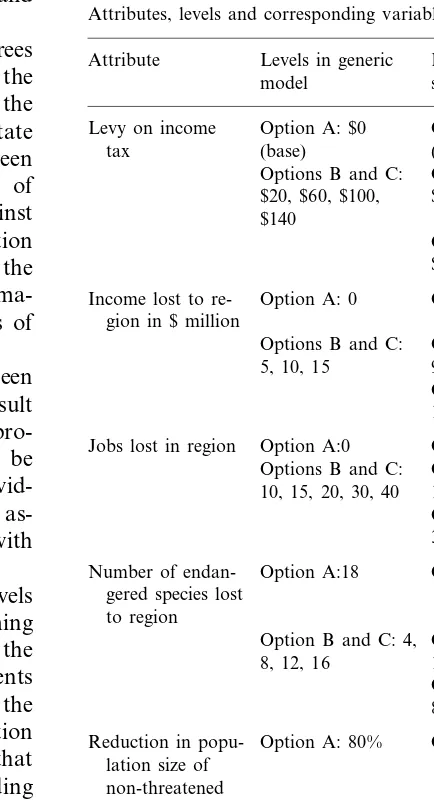
Table 1
Attributes, levels and corresponding variables
Attribute Levels in generic Levels in alt-spec. model model
Option A: $0
Levy on income Option A: $0
tax (base) (base)
Option B: $20, Options B and C:
$40, $60, $80
Income lost to re-gion in $ million
Options B and C: Option B: 5, 7,
5, 10, 15 9
Option C: 11, 13, 15 Option A:0
Jobs lost in region Option A:0 Options B and C: Option B: 10,
14, 18, 21, 24 10, 15, 20, 30, 40
Option C: 26, 30, 34, 37, 40 Number of endan- Option A:18 Option A:18
gered species lost
Reduction in popu- Option A: 80% Option A:80% lation size of
6The first set of focus groups involved two in Brisbane and a further two in Emerald. The second set involved two groups in Brisbane.
1 lists the attributes chosen.7
Note that environmental losses receive equal attention in the choice sets (and elsewhere in the questionnaire) to losses in jobs and regional in-come. Inclusion of the latter, ‘developmental’ at-tributes, is consistent with Portney’s observation (Portney, 1994) that people can have nonuse values for economic and social factors. The balanced environment – economy approach to information presentation addresses Blamey’s (1996, p. 128) concern that it is often futile to omit or downplay references to such outcomes ‘in the hope that respondents will not bring their own perceptions of such factors in as external variables’.
Citizens have general stances on environmental issues that they bring to the valuation situation, and implicit in these stances is a consideration of the relative importance of environmental factors and developmental factors. Omitting or downplaying the development side of the story not only leads some respondents to perceive the questionnaire to be biased, but also results in the elicitation of a blurred construct. The objective of environmental valuation is to estimate environmental consumer surplus. An alternative to seeking surplus validity is to seek a form of predictive validity pertaining to the maximum amount of money citizens are prepared to commit themselves to paying at a referendum (electoral validity). Developmental considerations and payment vehicle protests are invalid from the former perspective but valid from the latter. Unbalanced information presentation results in a blurred compromise between these two objectives. In this paper, we have attempted to maximise predictive WTP validity and to interpret WTP for environmental attributes within this light. To the extent that losses in regional income and employment are expected to be short-lived, lower impacts, or zero impacts, can be substituted into the
model as an approximation when estimating WTP and market share. Other stated preference studies that have included developmental benefits include Lockwood et al. (1994), Morrison et al. (1999).
The second round of focus groups focussed on the refinement of draft questionnaires. Some of the more important issues that emerged concerned the clarity of information; selection of photographic stimuli; cognitive burden (particularly as it relates to the number of choice sets); perceived bias of information presented; strategies for choice; and plausibility of attribute-combinations. Particular attention was also given to whether individuals interpreted information and questions in the way intended by the researchers. Different ways of introducing and explaining the choice modelling task were also explored.
Both generic and alternative-specific choice set configurations were trialed, and in some cases, in the same group.8Whilst some participants thought alternative-specific labels were a good idea, others were not so sure:
I think this puts a whole different spin on things....I think it makes the decision more realistic. E1
If you have that [label] on every single one, then people might just look at that… They might just go ‘I’ll pick the one with the most trees’. B2
A common tendency was to select the option with the label that most closely coincided with one’s environmental attitudes, and to see if significant reasons existed not to choose this alternative. The following statements illustrate how some individu-als used the labels to help structure their evaluations:
Straight away I thought yeah I do want to do something to increase it [the minimum permissi-ble tree retention] and I don’t mind paying some money. B3
8The particular group to which the verbatim quotes listed below correspond is indicated at the end of the citation for each quote, using the abbreviations B1 – 4 and E1 or E2. B2 thus refers to the second focus group conducted in Brisbane. 7Inclusion of an attribute pertaining to the percentage of
Putting the top line [labels] up there makes it a bit easier. B3
The final questionnaires were presented in the form of a small booklet with a colour cover, and a colour insert containing an attribute glos-sary for use when completing the choice sets. A map on the cover indicated the location of the Desert Uplands in Queensland, and proximity to nearby towns. A graphic artist finalised the pre-sentation of the questionnaire and pamphlet.
The levels assigned to the attributes listed in Table 1 were chosen such that the resultant at-tribute-space encompassed the vast majority of policy-relevant tree clearing options. Information regarding the ecological effects of different tree clearing options in the Desert Uplands, and consequent implications for humans, is ex-tremely limited. Information that could be gained regarding likely outcomes for jobs, re-gional income and threatened and non-threat-ened species was obtained from a variety of sources (summarised in Rolfe et al., 1997) and in consultation with experts. The high level of uncertainty regarding attributes such as impact on endangered species meant that the range of levels chosen was wider than one would expect to be the case with most policy options.
Because most respondents would expect greater tree clearing to involve worse environ-mental outcomes and better economic outcomes, attribute values in the labelled treatment were selected from alternative-specific sets of values. In other words, different policy labels were asso-ciated with different sets of outcomes. Table 1 lists the attribute levels applied to each option in each treatment and Fig. 1 illustrates the main differences between the two treatments.9 The ca-pacity to incorporate associations between at-tribute values and labels within the design of the experiment can be considered an advantage of the alternative-specific approach to choice set
design. Implausible combinations of attributes and labels are minimised as a result.10
To ensure that the attributes varied indepen-dently of one another, such that their individual effect on respondents’ preferences can be iso-lated, an orthogonal experimental design was used to assign attribute levels to alternatives. Fractional factorial designs were used to reduce the number of alternatives to a manageable level. Choice sets were constructed in such a way that orthogonality both between and within alternatives was ensured. To reduce implausibil-ity problems whilst at the same time increasing the balance between environmental and eco-nomic variables, a correlation between jobs lost and income lost was introduced by creating a composite 8 level attribute. Sixty-four choice sets were allocated to eight blocks of eight choice sets in each of the two versions, produc-ing a total of 16 versions of the questionnaire. An eight-level, orthogonal blocking variable was included as part of the experimental design, and used to generate the eight different blocks or versions of the survey. The purpose of the blocking factor is to insure that the eight blocks feature a balanced distribution of levels across all attributes, which ordinarily cannot be achieved using random assignment.
In both versions of the questionnaire, state-ments were included in the scenario with the purpose of further diffusing perceptions of im-plausible attribute combinations that may give rise to problematic response strategies. Respon-dents were told to ‘consider carefully the impli-cations of each tree-clearing option by looking at the numbers in the table. To keep matters simple, we do not describe how each option would work. Some implications which may seem a little odd are in fact quite possible…You will find some questions easier than others.’
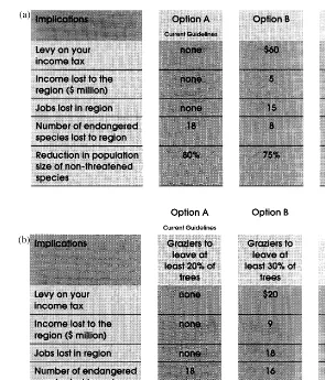
10Whether or not alternative-specific attribute levels are required clearly depends to a large extent on the nature of the information communicated by the labels. For example, labels based on biogeographic differences such as ‘The Desert Up-lands’ and ‘The Brigalow’ may not require alternative-specific attribute levels if respondents do not have strong a priori expectations regarding the relative magnitude of attribute lev-els for these regions.
Fig. 1. (a) An example of a generic choice set. (b) An example of an alternative-specific choice set.
7. Survey logistics
C. Neilsen McNair was contracted to adminis-ter the final questionnaire11
following a census style ‘drop-off and pick-up’ procedure. Thirty nodal points were randomly selected throughout the Brisbane metropolitan area. Each of these nodal points was used as a start point for the random selection of 16 respondent households. The final data set used for this paper contained 481 valid responses of which 241 employed the generic form of choice set presentation. Valid responses were obtained from :40% of all those approached.
8. Results
8.1. Specification issues
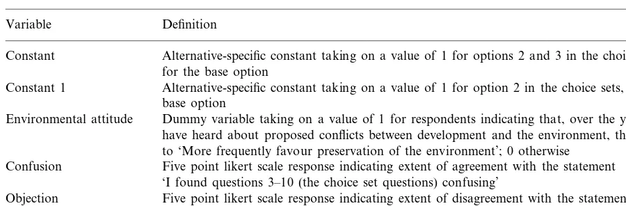
Tables 1 and 2 define the variables included in the choice models presented in this section. In contrast to the ‘environmental attitude’ variable, which provides a measure of respondents’ general stances on environmental issues, the ‘confusion’ and ‘protest’ variables relate to respondents’ reac-tions to the survey instrument.
Table 2
Non-attribute variable definitions Definition Variable
Constant Alternative-specific constant taking on a value of 1 for options 2 and 3 in the choice sets, and 0 for the base option
Constant 1 Alternative-specific constant taking on a value of 1 for option 2 in the choice sets, and 0 for the base option
Dummy variable taking on a value of 1 for respondents indicating that, over the years, when they Environmental attitude
have heard about proposed conflicts between development and the environment, they have tended to ‘More frequently favour preservation of the environment’; 0 otherwise
Five point likert scale response indicating extent of agreement with the statement Confusion
‘I found questions 3–10 (the choice set questions) confusing’
Five point likert scale response indicating extent of disagreement with the statement Objection
‘A tree levy is a good idea’
Dummy variable equalling 1 for the labelled treatment and 0 otherwise Version
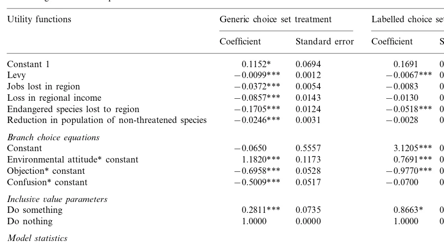
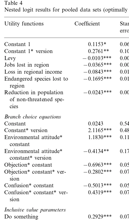
from a serious IIA violation in the generic, but not the labelled, treatment, using the Hausman and McFadden (1984) test. The violation was addressed by using a nested logit model with the two environmental improvement alternatives grouped in one branch and the status-quo or do-nothing option in the other. A branch-choice equation was specified in which respondents are first seen to choose between ‘doing something’ and ‘doing nothing’. The utilities of these two branches depends on an ASC and its interaction with environmental attitudes, self-reported confu-sion, and self-reported levy protest. Respondents choosing one of the pro-environment options are expected to have greener attitudes, and lower levels of confusion and protest, than those prefer-ring a continuation of the current tree cleaprefer-ring guidelines.12
At the second level of the nest, respondents are assumed to choose on the basis of the attributes of the alternatives. Although the labelled treat-ment did not present a significant IIA violation, the same nested structure was applied to facilitate model comparisons.
The second key issue is whether a generic model is appropriate for the alternative-specific treat-ment. The different labels and/or attribute ranges across alternatives may stimulate different mar-ginal utilities for the same attribute across
differ-ent alternatives. To this end, the labelled treatment was tested for compatibility for mod-elling using generic taste parameters (i.e. bj=1= bj=2=bj=3=b). The likelihood ratio test involves estimating both an unrestricted alterna-tive-specific model and a restricted generic model. The resultant LR statistic was 2.1, well below the critical values of 11.1 on 5 degrees of freedom (df). It appears that a generic model specification is appropriate for the alternative-specific treatment.13
Results for the final nested logit specifications are presented in Table 3. At the top level of the nest, all interactions with the ASC have the ex-pected signs and are highly significant in most cases. Respondents with a pro-environment orien-tation are more likely to choose one of the im-provement options than those with a pro-development perspective. Those who report being confused are more likely to choose the status quo, as are those who have a problem with the idea of a tree levy. Results pertaining to status-quo bias are discussed in more detail later in this section.
13This implies that the marginal attribute values are equal across options in the labelled treatment, even though the range of levels represented in each option is alternative-specific. It would appear that marginal utility is not diminishing at a significant rate over the range of attribute levels included in the questionnaire (Table 1).
Table 3
Nested logit results for separate data sets
Utility functions Generic choice set treatment Labelled choice set treatment Standard error Coefficient Standard error Coefficient
0.0694
Constant 1 0.1152* 0.1691 0.3218
0.0012
Levy −0.0099*** −0.0067*** 0.0018
0.0054 −0.0083
−0.0372*** 0.0092
Jobs lost in region
−0.0857***
Loss in regional income 0.0143 −0.0130 0.0271
0.0124 −0.0518***
−0.1705*** 0.0184
Endangered species lost to region
0.0031 −0.0028
Reduction in population of non-threatened species −0.0246*** 0.0061 Branch choice equations
Constant −0.0650 0.5557 3.1205*** 0.7698
0.1173 0.7691***
1.1820*** 0.1234
Environmental attitude* constant
−0.6958***
Objection* constant 0.0528 −0.9770*** 0.0554
0.0517 −0.0700 0.0509
Confusion* constant −0.5009***
Inclusi6e6alue parameters
0.0735 0.8663*
Do something 0.2811*** 0.4872
0.0000 1.0000
1.0000 0.0000
Do nothing Model statistics
1806 1840
n(choice sets)
−1547.388
LogL −1704.261
Adj rho-square (%) 26.7 18.2
* Denotes significance at the 10% significance level. ** Denotes significance at the 5% level.
*** Denotes significance at the 1% level.
8.2. Hypothesis 1
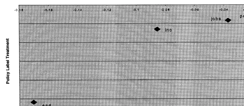
Before conducting a formal test of the equality of parameter vectors across the two treatments, it is useful first to examine visually the differences. Fig. 2 plots the attribute parameter vectors shown in Table 3. An examination of the plot suggests a fair degree of proportionality between the two vectors. Eyeing in a line of best fit in Fig. 2 indicates that the ratio of ‘generic’ to ‘labelled’ parameters is \1, implying that if the underlying taste parameters are the same, the generic data set has the lower variance. If inclusion of the policy labels results in greater heterogeneity with respect to choice strategies, one would expect variance to be higher in the labelled case.
The grid search technique of Swait and Lou-viere (1993) was applied to the stacked data sets. Results shown in Table 4 permit the hypothesis of equal attribute taste parameters across the two treatments to be tested. All terms involving the ASC are allowed to differ between treatments and
only the common attribute parameters are rescaled. The Swait – Louviere test can be used to test whether this reduced set of equality restric-tions provides as good a fit as the separate models shown in Table 3. The maximum log-likelihood for the rescaled data model corresponded to lL/ G=0.365, implying that the generic treatment has the lower variance. The likelihood ratio test statis-tic is
LR= −2[−3254.518
−(−1547.388+ −1704.261)]=5.74.
The critical value of thex2distribution is 11.07 at
the 95% significance level on 5 df. The hypothesis that the vector of common attribute parameters is equal across data sets thus cannot be rejected.
Fig. 2. Plot of attribute parameter vectors. LR= −2[−3273.947−(−3254.518)]=38.91
which well exceeds the critical value of 3.84 at the 95% CI.14
It appears that whilst the labelled treatment has stimulated respondents to base their responses more on the labels, and less on the attributes, than the generic treatment, underlying tastes with respect to the attributes do not differ significantly.
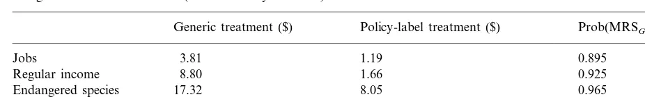
8.3. Hypothesis 2
Whilst the above results indicate no overall difference in the vector of attribute parameters across treatments, it is conceivable that one or more differences in marginal rates of substitution (MRS) may exist. In particular, the insignificance of several of the non-monetary coefficients in the labelled model is suggestive of lower implicit val-ues. The MRSs between the monetary attribute and each of the non-monetary attributes are pre-sented in Table 5 for each treatment. Note that the signs of the differences across treatments are as expected a priori in all cases. That is, the
labelled treatment is associated with a reduced importance of all non-monetary attributes. For example, a one million dollar increase in regional income is valued at $1.7 in the labelled treatment and $8.8 in the generic. Indeed, averaged over all four non-monetary attributes, the generic treat-ment produces MRSs that are more than four times higher than corresponding labelled MRSs.
Whilst the differences are statistically significant at the 95% level for both of the environmental attributes, using the Poe et al. test, the differences for regional income and jobs are significant at approximately the 90% significance level. Thus, whilst no significant differences in the parameter vectors containing the attributes were detected with the Swait – Louviere test, some differences in MRSs are apparent, and these have the expected sign. The use of alternative-specific labels and values appears to have reduced the implicit value of the attributes.
8.4. Hypothesis 3
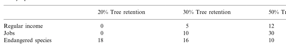
The third hypothesis takes on increased impor-tance given the results of the previous section. This hypothesis involves comparing the two treat-ments in terms of the overall welfare estimates generated for two specific scenarios. Eq. (10) is used to estimate compensating surplus associated with a movement from 20% tree retention to 30, 14An examination of results in Table 3 suggests that
or 50%, retention. These environmental improve-ments are associated with higher opportunity costs in the form of foregone regional income and jobs. Table 6 specifies the attribute values associ-ated with each of the policy options under consideration.
Using Eq. (10) to estimate the welfare implica-tions of moving from 20 to 30% retention pro-duces mean welfare estimates of $119 and $83 per respondent (one-off), respectively, for the labelled
and generic treatments. These values are calcu-lated at the mean values for protect, confusion and objection. Both the ASCs and the attributes are included when calculating Vi0 and Vi1.
An examination of the magnitude of the ASC terms indicates considerable unobserved and sys-tematic utility. In the generic treatment, for exam-ple, the environmental improvement options have an unobserved utility of – 2.9 relative to the cur-rent guidelines. This is suggestive of the occur-rence of status-quo biases similar to those reported by Adamowicz et al. (1998). When mini-mum rather than average levels of objection and confusionare substituted, the unobserved utility of the improvement options increases to – 0.66.15 In the labelled treatment, the improvement options have an unobserved utility of +0.4175 relative to the current guidelines, at the average levels of confusion and objection, and +2.4 at the mini-mum of these variables. Thus, the environmental improvement alternatives are associated with greater unobserved utility in the labelled treat-ment than the generic treattreat-ment.
Potentially offsetting the positive utility associ-ated with the pro-environmental labels in the labelled treatment is the lower contribution of utility from the attributes in this treatment. A Poe et al. test was conducted to determine whether the $119 estimate is significantly higher than the $83 estimate. The two estimates were not found to be significantly different (P=0.41).
These welfare estimates represent net improve-ments in the mean welfare of Brisbane residents resulting from tighter tree clearing guidelines in the Desert Uplands. They are net values in the sense that they take into account the losses experi-enced by Brisbane residents resulting from changes to the economy of the Desert Uplands region. It is possible to recalculate the estimates for the case in which only the above environmen-tal improvements are considered. When employ-ment and income effects are held constant and at the levels specified for the 20% tree retention Table 4
Nested logit results for pooled data sets (optimally scaled) Coefficient Standard
Constant 1* version 0.1081
−0.0103*** 0.0011 Levy
−0.0365***
Jobs lost in region 0.0053
Loss in regional income −0.0843*** 0.0141 Endangered species lost to −0.1695*** 0.0120
region
0.0031 Reduction in population −0.0243***
of non-threatened
spe-Environmental attitude* 1.1830*** 0.1173 constant
0.1702 Environmental attitude* −0.4134**
constant* version
Objection* constant −0.6963*** 0.0528 Objection* constant* ver- −0.2802*** 0.0765
sion
Confusion* constant −0.5013*** 0.0517 Confusion* constant* ver- 0.4319*** 0.0725
sion
Inclusi6e6alue parameters
0.2929***
Do something 0.0729
Do nothing 1.0000 0.0000
Model statistics
0.365 Optimal scale ratio
n(choice sets) 3646
LogL −3254.518
Adj rho-square (%) 22.4
* Denotes significance at the 10% significance level. ** Denotes significance at the 5% level.
*** Denotes significance at the 1% level.
Table 5
Marginal rates of substitution (with monetary attribute)
Policy-label treatment ($) Prob(MRSG−MRSL\0)
Generic treatment ($)
1.19
Jobs 3.81 0.895
Regular income 8.80 1.66 0.925
Endangered species 17.32 8.05 0.965
0.39 0.965
2.51 Population species
scenario, the welfare estimates become $106 and $108, respectively. Again, the difference is not statistically significant (P=0.49). The latter esti-mates should only be considered an approxima-tion. Whilst contributions to utility from the job and regional income attributes can be controlled for, the ASC terms will to some extent reflect attitudes to employment, which cannot be isolated.
In the case of 50% rather than 20% tree reten-tion, the mean welfare estimates are $107 and $84, respectively, for the labelled and generic treat-ments. The difference was not found to be signifi-cantly different using the Poe et al. test (P=0.44). When the employment and income effects associ-ated with the environmental improvement are as-sumed to be zero, the estimates increase to $146 and $155, respectively, which are still not statisti-cally different.
It appears that the labelled and generic treat-ments do not produce significantly different esti-mates of consumer surplus for the scenarios considered in this section.
9. Conclusion
A key issue that arises when conducting CM studies is whether to present choice sets in a generic or alternative-specific form. The preferred approach will often depend on the objective of the study. When the objective is to estimate attribute values or marginal rates of substitution the generic approach will tend to be preferred. This approach has the potential to elicit more discern-ing trade-off information. An assumption that more informed preferences are in some way
desir-able is implicitly made when designing most SP questionnaires.
When the objective is to predict the amount of money people would actually pay to obtain a given policy alternative, and meaningful labels for the alternatives are apparent, the labeled ap-proach will tend to be preferred. This apap-proach can be expected to result in greater predictive validity when the inclusion of policy or other labels increases correspondence between emo-tional triggers and other cues embedded within the questionnaire and those that would be embed-ded within a true market or electoral context. When the objective is to estimate consumer sur-plus, the preferred approach is less clear and depends on the fit between the circumstances de-scribed in the questionnaire and those relevant to the environment in which consumer surplus would be experienced.
The two approaches to choice set construction were compared in this study in the context of a case study involving the possibility of increased retention of remnant vegetation in the Desert Uplands of Central Queensland. Results indicate that whilst the mean unobserved utility compo-nent differs across the generic and alternative-spe-cific treatments, as reflected by the ASCs and their interactions, the vectors of attribute taste parame-ters do not differ significantly when scale differ-ences are incorporated.
Table 6
Policy options used in welfare estimation
30% Tree retention
20% Tree retention 50% Tree retention
5
Regular income 0 12
Jobs 0 10 30
16
Endangered species 18 10
50
80 35
Population species
unless this alternative is deemed unacceptable in terms of the one or two most important attributes (levy and impact on endangered species). The fact that the two attribute parameter vectors rescale is in part a function of the relatively high standard errors of the parameters in the alternative-specific treatment, and the fact that three of the five attributes add little to explanatory power.
Differences between the treatments also emerged with respect to marginal rates of substi-tution. In general, implicit prices for the attributes were lower in the alternative-specific treatment, a result that is consistent with the response strategy suggested above.
Importantly, however, no statistically signifi-cant differences in welfare estimates were de-tected, when estimated for two different environmental improvement options. This sug-gests that the inclusion of alternative-specific pol-icy labels and levels may have simply redistributed the source of the utility in terms of the attribute part worths and the ASC terms. The inclusion of policy labels appears to have shifted respondents’ attention from the attributes to the labels, with the overall utility implications of a given policy option remaining unchanged. This is a positive result as far as the convergent validity of CM is concerned.
Acknowledgements
The research reported in this paper was funded by the the Land and Water Resources Research and Development Corporation (LWRRDC), En-vironment Australia, Queensland Department of Primary Industries (QDPI) and the Queensland Department of Natural Resources (QDNR).
References
Adamowicz, W., Louviere, J., Williams, M., 1994. Combining revealed and stated preference methods for valuing envi-ronmental amenities. J. Environ. Econ. Manag. 26, 271 – 292.
Adamowicz, W.L., Swait, J., Boxall, P., Louviere, J., Williams, M., 1996. Perceptions versus objective measures of envi-ronmental quality in combined revealed and stated prefer-ence models of environmental valuation. J. Environ. Econ. Manag. 32, 65 – 84.
Adamowicz, W., Boxall, P., Williams, M., Louviere, J., 1998. Stated preference approaches for measuring passive use values: choice experiments and contingent valuation. Am. J. Agric. Resour. Econ. 80, 64 – 75.
Ben-Akiva, M., Lerman, S.R., 1985. Discrete Choice Analysis: Theory and Application to Travel Demand. MIT Press, Cambridge.
Blamey, R.K., 1996. Citizens, consumers and contingent valu-ation: clarification and the expression of citizen values and issue opinions. In: Adamowicz, V (Ed.), Forestry, Eco-nomics and the Environment. CAB International, Walling-ford, UK.
Blamey, R.K., Gordon, J., Chapman, R., 1999. Choice mod-elling: assessing the environmental values of water supply options. Aust. J. Agric. Res. Econ. 43, 337 – 357. Blamey, R.K., Rolfe, J.C., Bennett, J.W., Morrison, M.D.,
1997. Environmental Choice Modelling: Issues and Quali-tative Insights, Research Report No. 4. Department of Economics and Management, ADFA.
Boxall, P.C., Adamowicz, W.L., Swait, J., Williams, M., Lou-viere, J., 1996. A comparison of stated preference methods for environmental valuation. Ecol. Econ. 18, 243 – 253. Carson, R.T., Louviere, J.J., Anderson, D.A., et al., 1994.
Experimental analysis of choice. Marketing Letts. 5, 351 – 368.
Choi, K.-H., Moon, C.-G., 1997. Generalized extreme value model and additively separable generator function. J. Econom. 76, 129 – 140.
Daganzo, C.F., Kusnic, M., 1993. Two properties of the nested logit model. Transp. Sci. 27, 395 – 400.
Hanemann, W.M., 1984. Applied Welfare Analysis with Qual-itative Response Models, Working Paper 241. University of California, Berkeley, CA.
Hausman, J., McFadden, D., 1984. Specification tests for the multinational logit model, Econometrica, September, pp. 1219 – 1240.
Hanley, N., MacMillan, D., Wright, R.E., Bullock, C., Simp-son, I., ParsisSimp-son, D., Crabtree, B., 1998a. Contingent valuation versus choice experiments: estimating the benefits of environmentally sensitive areas in Scotland. J. Agric. Econ. 49, 1 – 15.
Hanley, N., Wright, R.E., Adamowicz, V., 1998b. Using choice experiments to value the environment. Environ. Resour. Econ. 11, 413 – 418.
Hensher, D.A., Johnson, L.W., 1981. Applied Discrete Choice Modelling. John Wiley, New York, 468 pp.
Herriges, J.A., Kling, C.L., 1997. The performance of nested logit models when welfare estimation is the goal. Am. J. Agric. Econ. 79, 792 – 802.
Kling, C.L., Thomson, C.J., 1996. The implications of model specification for welfare estimation in nested logit models. Am. J. Agric. Resour. Econ. 78, 103 – 114.
Krinsky, I., Robb, A.L., 1986. On approximating the statisti-cal properties of elasticities. Rev. Econ. Stat. 68, 715 – 719. Lancaster, K., 1966. A new approach to consumer theory. J.
Polit. Econ. 74, 132 – 157.
Lancaster, K., 1991. Modern Consumer Theory. Edward El-gar, Brookfield.
Lockwood, M, Loomis, J., DeLacy, T., 1994. The relative unimportance of a non-market willingness to pay for tim-ber harvesting. Ecol. Econ. 9, 145 – 152.
Louviere, J.J., 1988. Analyzing Decision Making: Metric Con-joint Analysis. Sage Publications, Newbury Park. McCosker, J.C., Cox, M.J., 1996. Central Brigalow
Biore-gional Conservation Strategy Report. Australian Nature Conservation Agency, Canberra.
McFadden, D., 1978. Modeling the choice of residential loca-tion. In: Karlquist, A., Lundquist, L., Snickars, F., Weibull, J.W. (Eds.), Spatial Interaction Theory and Plan-ning Models. North-Holland, Amsterdam, pp. 75 – 96. Mitchell, R.C., Carson, R., 1989. Using Surveys to Value
Public Goods: The Contingent Valuation Method. Re-sources for the Future, Washington.
Morrison, M, Blamey, R.K., Bennett, J.W., Louviere, J., 1996. A Comparison of Stated Preference Techniques for Esti-mating Environmental Values, Research Report No. 1. Department of Economics and Management, ADFA, p. 30.
Morrison, M.D., Bennett, J.W., Blamey, R.K., 1997. Design-ing Choice ModellDesign-ing Surveys UsDesign-ing Focus Groups: Re-sults from the Macquarie Marshes and Gwydir Wetlands Case Studies, Research Report No. 5. Department of Economics and Management, ADFA.
Morrison, M.D., Bennett, J.W., Blamey, R.K. 1999. Valuing improved wetland quality using choice modelling. Water Resour. Res. (in press).
Opaluch, J.J., Swallow, S.K., Weaver, T., Wessells, W., Wichelns, D., 1993. Evaluating impacts from noxious facil-ities: including public preferences in current siting mecha-nisms. J. Environ. Econ. Manag. 24, 41 – 59.
Poe, G.L., Severance-Lossin, E.K., Welsh, M.P., 1994. Mea-suring the difference (x(y) of simulated distributions: a convolutions approach. Am. J. Agric. Econ. 76, 904 – 915. Poe, G.L., Welsh, M.P., Champ, P.A., 1997. Measuring the difference in mean willingness to pay when dichotomous choice contingent valuation responses are not independent. Land Econ. 73, 255 – 267.
Portney, P.R., 1994. The contingent valuation debate: why economists should care. J. Econ. Perspect. 8, 3 – 17. Rolfe, J., Bennett, J. 1996. Valuing International Rainforests:
A Choice Modelling Approach. Paper presented at the 40th Annual Conference of the Australian Agricultural Economics Society, Melbourne, February, pp. 11 – 16. Rolfe, J, Blamey, R.K., Bennett, J.W., 1997. Remnant
Vegeta-tion and Broadscale Tree Clearing in the Desert Uplands Region of Queensland, Research Report No. 3. Depart-ment of Economics and ManageDepart-ment, ADFA.
Rossiter, J.R., Percy, L., 1997. Advertising Communications and Promotion Management. McGraw Hill, Sydney. Simon, H.A., 1955. A behavioural model of rational choice. Q.
J. Econ. 69, 99 – 118.
Swait, J., Louviere, J., 1993. The role of the scale parameter in the estimation and comparison of multinomial logit mod-els. J. Marketing Res. 30, 305 – 314.
Swait, J., Louviere, J., Williams, M., 1994. A sequential ap-proach to exploiting the combined strengths of SP and RP data: application to freight shipper choice. Transportation 21, 135 – 152.
Train, K., 1986. Qualitative Choice Analysis, Theory, Econo-metrics and an Application to Automobile Demand. MIT Press, London.
Train, K.E., McFadden, D.L., Ben-Akiva, M., 1987. The demand for local telephone service: a fully discrete model of residential calling patterns and service choices. Rand J. Econ. 18, 109 – 123.