www.elsevier.com/locate/econedurev
Evaluating performance in Chicago public high schools in
the wake of decentralization
Shawna Grosskopf
a,*, Chad Moutray
baOregon State University, Economics Department, Corvallis, OR 97331-3612, USA bRobert Morris College, 401 South State Street, Chicago, IL 60605, USA
Received 15 September 1996; accepted 27 January 1999
Abstract
This research analyses the changes in performance for Chicago high schools between 1989 and 1994 following the introduction of site-based management in 1988. The purpose of this paper is to assess whether this decentralization improved performance or not. We modeled the change from centralized to decentralized control following Grosskopf, Hayes, Taylor & Weber, 1999 (Anticipating the consequences of school reform: a new use of DEA, Management
Science), and used cost indirect output distance functions to model decentralized control. Malmquist productivity index
results show very little improvement in productivity with sample achieved improvements off-setting realized declines. Second stage regression results, though, provide some evidence of small improvements in efficiency over this time period. Thus, the overall results are mixed.2001 Elsevier Science Ltd. All rights reserved.
JEL classification: I21; D24
Keywords: Chicago; Data envelopment analysis (DEA); Education performance; Educational finance; Efficiency; Productivity; Resource allocation
1. Introduction
In the November 7, 1987 issue of the Chicago Sun
Times, William Bennett, then Secretary of Education,
declared the Chicago public school system to be the “worst in America”. According to Hess (1991), about one half of Chicago’s high schools scored in the lowest one percent on the ACT of all US high schools, and sixty to seventy percent of elementary students were below national norms on reading tests.
Perhaps in response, the Illinois legislature passed the Chicago School Reform Act of 1988, which dramatically changed the organization of Chicago public schools. Before this reform, all of the almost 600 schools in
* Corresponding author.
E-mail addresses: [email protected] (S. Grosskopf), [email protected] (C. Moutray).
0272-7757/01/$ - see front matter2001 Elsevier Science Ltd. All rights reserved. PII: S 0 2 7 2 - 7 7 5 7 ( 9 9 ) 0 0 0 6 5 - 5
Chicago were in one school district governed centrally by the Chicago Board of Education. The 1988 reform introduced site-based management, which returned decision-making control to the individual schools. Each school acquired its own elected local school council, which could make decisions concerning principal evalu-ation and selection, budgeting and planning.
must attend summer school, etc. Although the local school councils are nominally in place, in effect the Chicago public schools have been returned to a high degree of central control.
The purpose of this paper is to assess whether the earl-ier experiment in site-based management really failed to improve performance in Chicago’s high schools.1 We
employ a stylized model of schools under site-based management as the building blocks for our performance measures. One of the features of site-based management is the devolution of control over the budget to the indi-vidual schools and their elected councils. The budget is given in total, but the local council is given discretion over how to spend it. To capture this basic element of site-based management we use a cost indirect output dis-tance function to model individual schools. This is essen-tially a multiple output production function with a budget constraint. The idea is that the local council’s goal is to maximize school outcomes, given the technological possibilities, and given their budget. How to allocate the budget across inputs is a choice variable in this problem. We use these building blocks to compute productivity changes over the 1989–94 time period. This index, the Malmquist productivity index, does not require output prices to aggregate outputs and does not presume efficiency or profit-maximizing behavior. The Malmquist productivity index also provides information on the sources of productivity change, which include changes in efficiency and changes in the frontier (innovation). This will prove useful, for instance, in determining if the decentralized system under reform became more (less) efficient as a result of the change, or whether these changes actually shifted the frontier.
We analyze the changes in performance of Chicago high schools between 1989 and 1994 using data obtained from both the Illinois State Board of Education and the Chicago Panel on Public School Policy and Finance. We find that performance in Chicago public high schools was mixed over the 1989–94 reform period. Roughly half of the schools improved (slightly), while roughly half showed declines in productivity over this time per-iod. Higher spending per pupil was associated with lower productivity in our sample.
2. Background
Smylie et al. (1994) provide a description of the Chicago site-based management program:
In 1989, Chicago’s public schools began the nation’s “most radical” experiment in school decentralization.
1 We do not include Chicago primary level public schools in our analysis due to data limitations.
Each of the city’s nearly 600 schools acquired its own governing board in the form of an elected local school council (LSC). Six of each council’s 11 members are parents and community representatives. Armed with the power to hire and fire their building principals, these councils also acquired significant, previously centralized controls over school-site budgets, curric-ula, and school-improvement planning.
Prior to reform, all Chicago schools were in one school district (District 299) and the Chicago Board of Education coordinated all schools and made most of the decisions.2
After reform local school councils were formed; they consisted of parents, community members, teachers, the school principal, and a student. Except for the principal, these members were elected every two years. Easton & Storey (1994) describe the functions of the LSC mem-bers as follows.
They have major decision-making power in three important areas: principal evaluation and selection, budgeting, and school improvement planning. LSCs are also charged with making recommendations on textbooks, advising the principal on attendance and disciplinary policies, and evaluating the allocation of staff in the school.
The motivation for decentralization was to allow tea-chers and parents to make crucial decisions affecting their students and children.3 Those who actually were
involved personally with the school would make decisions regarding school policies, curricula, and dis-cretionary funding. By empowering teachers and parents, real “local control” could be established. Following Garms, Guthrie & Pierce (1978), parents are more likely to participate in their children’s education when they have a voice in the decisions concerning their individual school. This participation was expected to improve edu-cational outcomes.
After the Chicago School Reform Act of 1988, Chicago schools also regained access to funds from Title 1 (formerly Chapter 1). These are federal funds distrib-uted by the state of Illinois based on low-income student enrollment. Before the reform, according to Rosenkranz
2 Under both the old and the reform system, there are twenty elementary and three high school subdistricts. Each subdistrict has a superintendent responsible for nineteen and thirty-eight schools.
(1994) “. . . the Chicago panel revealed that one third of the targeted funds were being misappropriated and diverted away from schools into central office bureau-cratic positions”. After the Chicago School Reform Act of 1988, more of these funds reached the individual schools, which were then able to decide how these funds would be used. In the 1993–94 school year, new dis-cretionary funds amounted to $491,000 for elementary and $849,000 for high schools on average.4
Current evidence on the impact of these reforms—in Chicago and elsewhere—is mixed. For instance, Eub-anks & Levine (1983) describe improvements in test scores in both Milwaukee and New York after school-based planning committees were instituted to encourage more parent–teacher cooperation. Similarly, Rogers & Chung (1983) find improvements in reading and math scores in New York between 1970 and 1979. Meanwhile, Sickler (1988a,b) notes that standardized test scores rose and student and teacher absenteeism fell when the ABC District in Cerritos, California gave teachers more con-trol over curriculum. While Steward (1991) finds posi-tive gains in ACT scores at Tilden High School during the first few years after the Chicago site-based manage-ment reform, Bryk et al. (1994) find no significant gains in improvement on the Iowa Test of Basic Skills for grades one through eight in Chicago. In reviewing the literature, Malen, Ogawa & Kranz (1990) conclude that there is no consistent link between school-based manage-ment and student achievemanage-ment.
Downes & Horowitz (1994) provide some econo-metric evidence concerning the results of Chicago’s 1988 reform on outcomes. The authors analyze test score data from the Illinois Goals Assessment Program (IGAP) and ACT to determine if decentralization positively or nega-tively affected student performance. They conclude that IGAP reading test scores for grades 3, 6, and 8 decreased relative to other schools in the state after reform; on the other hand, post-reform high school graduation rates and
4 In addition to site-based management, many Chicagoans want to establish other types of reforms. For instance, the Illi-nois legislature has considered a plan that would establish a pilot voucher program similar to the one in Milwaukee. Accord-ing to Harp (1995), this plan would shift $5 million from the Chicago school district’s budget to provide a $2,500 voucher to low-income parents. The parents could then opt for a private or parochial school. The pilot program would start in the His-panic neighborhoods of Pilsen and Little Village. This legis-lation passed the Illinois Senate, but it failed to get enough votes in the Illinois House in May 1995. Thus, its future is uncertain. The second reform is the establishment of charter schools that would allow individual schools, by escaping many state rules and regulations, to experiment with new teaching techniques. According to Dizon & Pearson (1996), Governor Jim Edgar signed the bill into law creating 15 charter schools in Chicago, 15 in the suburbs, and 15 downstate.
ACT scores have increased relatively. The authors find lower outcomes after reform for those Chicago schools with a larger percentage of students with limited English proficiencies (LEP) and a larger percentage of students who qualify for low-income school lunch assistance. Thus, they write the following:
The negative relationship between post-reform suc-cess and the relative size of a school’s at-risk popu-lation appears to imply that decentralization may not be the answer for urban school systems, since the result seems to indicate individual Chicago schools failed to benefit from additional control over Chapter 1 funds.
Despite the political and social momentum that appears to be building around changing the status quo, there is still very little empirical evidence on the success of educational reform in improving school outcomes. There are several reasons for this. One reason is that the first experiments in reform that do exist are recent, and therefore, there is little post-reform data. Another prob-lem is the difficulty in measuring performance. For instance, it is not obvious how to measure outputs, and it is not clear how best to model exogenous factors such as the role of the family. This measurement debate has been well-documented in the literature; it is perhaps best summarized in Hanushek (1986).
In this paper, we propose to address some of these problems and measure the performance of Chicago high schools during the site-based management experiment, i.e., 1989–1994. In terms of a measure of performance, we follow Grosskopf, Hayes, Taylor & Weber (1999) and actually measure potential gains from allowing for the type of decentralized decision-making that should occur under site-based management. This is achieved by using cost indirect output distance functions (due to Shephard (1953, 1974)) which we use to construct our productivity measures. One advantage of this model and technique is that it readily allows for multiple outputs or educational outcomes and explicitly includes a budget constraint. As educational outputs we include measures of changes in test scores which have been corrected for student characteristics and previous performance, i.e., we include measures of the value-added in terms of test scores due to the school. We also include two other mea-sures of school success (which the current Daley-led sys-tem also employs as school performance benchmarks): graduation rates and degree of truancy. We turn next to a discussion of our performance measures.
3. Performance measurement
con-trol over their budgets. We follow Grosskopf et al. (1999) and use indirect output distance functions to achi-eve that goal.
Shephard type distance functions are generalizations of a production function to the multiple output case.5
They provide a complete description of technology and also have a built-in interpretation as a performance meas-ure: they are reciprocals of Farrell (1957) technical efficiency measures. We begin with what we call the direct output distance function. In terms of notation, let
x denote a N-dimensional non-negative vector of inputs,
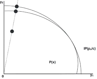
which are used to produce a M-dimensional vector of non-negative outputs, y. The most basic description of technology in this multiple-output case is the production possibilities set, which we denote P(x). It is the set of all outputs producible from the given input vector x.
The formal definition of the direct output distance function is:
Do(x,y)5min
q
{q.0:y/qeP(x)} where xPRNt, yPRMt. (1)
In this definition, 1/qis the proportion that the vector of outputs y could feasibly be expanded to reach the frontier or boundary of the production possibilities set.
This is illustrated for a two output case in Fig. 1. Point
A represents a school which is using input vector x, but
is producing an output vector that is interior to the boundary of the production possibilities set, P(x); i.e., school A is using the given input vector x, but is not achieving maximum potential output. The value of the direct output distance function for this observation can be written as:
Do(x,y)5
0A
0U. (2)
Thus, in order to expand an inefficient observation, such as A, up to the frontier, the value of the direct output distance function would have to be smaller than one. Note that observations on the boundary of the set would have values equal to one, i.e., no further scaling of out-puts are possible.
More generally, the production possibilities set (or output set) can be characterized as:
P(x)5{y:Do(x,y)#1}. (3)
Under site-based management, however, individual schools have some control over input choices, as long as they do not exceed their budgets. With this in mind, we follow Grosskopf et al. (1999) and use cost indirect
5 As shown by Shephard (1953), distance functions also satisfying nice duality properties.
output distance functions to model education production under site-based management. Following Shephard (1974), the cost indirect output distance function is defined as follows:
IDo(pv/c,y)5min
l
{l.0:y/lPIP(pv/c)}. (4)
In this equation pv represents the vector of variable
input prices, and total variable cost is denoted as c. The indirect production set, IP(pv/c), illustrates the
combi-nations of outputs which are feasible given the budget constraint. This can be expressed as:
IP(pv/c)5{y:yPP(x), pvxv#c}. (5)
Instead of variable inputs being given as in the direct output distance function, they are chosen subject to satis-faction of the budget constraint. Thus, the indirect dis-tance function helps model the decentralized control over input choices which is a keystone of site-based manage-ment.
Analogous to the direct output distance function, 1/l is the proportion that the vector of outputs y could feasi-bly be expanded to reach the (indirect) production possi-bilities frontier. In addition, the indirect output distance function at observation A equals:
IDo(pv/c,y)5
0A
0T. (6)
Returning to Fig. 1, in order for observation A to be expanded up to the frontier, the value of the indirect out-put distance function would be smaller than one. Schools are efficient in the Farrell sense for both direct and indirect output distance functions if they equal one.
Since, at least in principle, Chicago’s site-based man-agement reforms decentralized the overall budget decisions of the individual schools, the individual schools had more control over the choice of the appropri-ate choice of inputs subject to their budget constraint. Decentralization, it was hoped, would increase the level of potential output, which in our model is illustrated by the fact that the indirect output set is “larger than” the direct output set, giving the school more choice in terms of inputs.
In estimating the distance functions, we use the same techniques employed in data envelopment analysis (DEA). This approach uses linear programming tech-niques to form IP(pv/c) and measure the “distance” to
Fig. 1. Direct and indirect output distance functions. Source: Grosskopf et al. (1999).
compute the indirect output distance functions are included in Appendix A.6
The discussion up to this point has concentrated on a static analysis of technical efficiency; next we turn to a comparative static model, which computes performance over time, namely productivity change. Specifically, we begin with the Malmquist productivity index as described in Fa¨re, Grosskopf, Lindgren & Roos (1989) and Fa¨re & Grosskopf (1994) but modified to the indirect case as in Fa¨re et al. (1985). The Malmquist productivity index was first proposed by Caves, Christensen & Diew-ert (1982). Computations in a DEA framework and the technique of separating this index into technical inno-vation and efficiency change was later developed by Fa¨re et al. (1989). This procedure has been applied to many
6 Several recent studies have used DEA type approaches in assessing the technical efficiency of individual school districts. For example, studies applying DEA to education include Bessent & Bessent (1980); Bessent, Bessent, Kennington & Reagan (1982) and Charnes et al. (1978). Later, Jesson, Mays-ton & Smith (1987) and Barrow (1991) used DEA to analyze local education authorities in England. In a more recent study, McCarty & Yaisawarng (1993) measure technical efficiency in New Jersey schools. Meanwhile, Fare, Grosskopf & Weber (1989) concentrate on Missouri schools, and Grosskopf et al. (1999) compute the potential gain from deregulating Texas school districts.
topics; for example, Fa¨re, Grosskopf, Lindgren & Roos (1992) study productivity changes in Swedish phar-macies, and Fa¨re, Grosskopf, Norris & Zhang (1994) analyze productivity growth in industrialized countries. The aforementioned studies used a Malmquist index based on direct output distance functions. Since we will be analyzing productivity of Chicago schools under site-based management, we instead use a Malmquist index based on indirect output distance functions, following Fa¨re et al. (1985).7
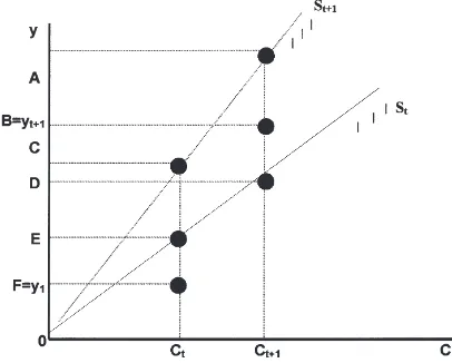
Fig. 2 illustrates the concept of the Malmquist indirect productivity index assuming constant returns to scale. This diagram uses two technologies, Stand St+1, for two
time periods. The total cost of the variable inputs is again denoted as c. In this situation, all points lying below the technology St are technically inefficient; point F is an example of such an observation. Given the budget con-straint, the production set Stis defined as:
St5{(xt,yt):ytPIPt(ptv/ct)} where xtPRN+,ytPRM+. (7)
Time period t+1 provides another technology St+1
which lies above the first; thus, more output can be achi-eved with the same budget. Point B is an example of a technically inefficient observation at time period t+1.
Fig. 2. Malmquist indirect output-based productivity index.
The Malmquist productivity index computes the change in performance between t and t+1.
Given the output distance functions defined earlier, Caves et al. (1982) (CCD) proposed measuring pro-ductivity as the ratio of two distance functions at periods
t and t+1. CCD make the assumption that there is no technical inefficiency. Fa¨re et al. (1989) relax this assumption and express the output-based Malmquist pro-ductivity index as the geometric mean of two CCD indexes. Following Fa¨re & Grosskopf (1994) and Fa¨re et al. (1985), the indirect version of this index is:
IMo((pv/c)t+1,yt+1,(pv/c)t,yt) (8)
This geometric mean can be decomposed into two parts as:
Using this formulation, it is possible to isolate both the change in technical efficiency and the change in tech-nical innovation between the years t and t+1. The first term in Eq. (10) is the efficiency change measure. The square root term is the technical change portion. In geo-metric terms using Fig. 2, the indirect version of the Malmquist productivity index can be given as:
IMo( )5
If there is an improvement in technical efficiency over the two time periods, the Malmquist index will be greater
than one; a decline in productivity will produce an index that is less than one. The two component measures have a similar interpretation. As mentioned earlier we use DEA type techniques to estimate the indirect output dis-tance functions used to construct the productivity index. These productivity indexes allow us to look at whether performance under site-based management improved over the 1989–94 time period.
To conclude the discussion on the Malmquist pro-ductivity index, Fa¨re & Grosskopf (1990) cite its advan-tages over the Fisher or To¨rnqvist indexes. First, since both the Fisher and To¨rnqvist indexes require price and quantity data on both inputs and outputs, they might be difficult to use in education and other industries where output prices, for example, are not available. The Malmquist indirect productivity index, on the other hand, does not require output price data which makes it the more practical choice for education research. The second advantage is the fact that, unlike the Fisher and To¨rnqvist indexes, the Malmquist index can be applied to cases where profit maximization is not presumed to prevail.
4. Chicago high school data
Like many states, Illinois publishes a “school report card” every year to assess the performance of each school. All data in this paper are taken from the Illinois State Board of Education’s School Report Card except for data on teachers and administrators. The number of teachers and administrators for each school and the aver-age teacher and administrator salaries are from the Chicago Panel on Public School Policy and Finance. Since the Chicago Panel’s data starts in fiscal 1989, Chicago’s high schools will be assessed here using the data for the fiscal years 1989 through 1994.8
Several studies argue that the most appropriate method of measuring educational output is the value-added effects of school outcomes. The idea is that the school should be credited with producing improvements in edu-cational outcomes above and beyond previous test per-formance and the effects outside the control of the school including student background and parental input. Examples of this approach include Aitken & Longford (1986), Boardman & Murnane (1979), Hanushek (1986) and Hanushek & Taylor (1990). In this paper we use the marginal effects method described in Aitken & Longford
(1986), Hanushek & Taylor (1990) and Grosskopf, Hayes, Taylor & Weber (1998).9
This is achieved by regressing test scores on measures of previous performance and other exogenous factors. Specifically, the following ordinary least squares regression is computed for each fiscal year t for the two ACT tests, math and English:
TESTi,t5b01b1TESTi,t−11b2LEPi,t1b3LOWi,t (11)
1b4MOBi,t1ei,t
In this equation TESTi,tis the average ACT score for a particular high school for fiscal year t. Similarly,
TESTi,t21is a school’s average ACT score for the
pre-vious fiscal year.10 LEP
i,t is the limited English pro-ficiency rate, and LOWi,tis the rate of students who qual-ify for school lunch assistance. MOBi,t is the mobility rate for each school and each fiscal year. According to the Illinois State Board of Education, this rate can exceed 100 percent since it counts both the number of students entering and exiting a school during the year. Finally, the estimated residual, ei,t, captures the average value-added effects. This model was estimated separately for ACT math and English scores.
Using this method of estimated value-added effects, school districts that add less than the average of all Chicago high schools will have negative output meas-ures. Following Grosskopf et al. (1998), these residuals are normalized in the following manner to ensure non-negative values.
YTESTi,t5(TESTt1ei,t)∗TAKERSi,t (12)
This measure of value-added effects for each school multiplies the number of students taking the ACT exams (TAKERSi,t) times the sum of the average ACT test score in either English or math for all Chicago high schools (
TESTt) and the value-added residuals from Eq. (11) for each fiscal year (ei,t). Adding the mean to the residual eliminates negative values. Multiplying by the number
9 For the purposes of comparison, we also estimated our model using levels rather than value-added effects. This did not produce significantly different results, and they are not reported here.
10 It would be preferable to regress the ACT English and math scores against some other exam, such as the tenth/eleventh grade Illinois Goals Assessment Program (IGAP) test scores. This would allow us to truly measure the value-added effects of a specific group of students. This is not possible, though, since the IGAP scores are not available for all of the years studied. Thus, Eq. (12) serves as a proxy for these value-added effects. We note that using ACT scores means that our measure ignores the value added to students who don’t take the ACT test.
of test takers gives us an aggregate measure of the value-added in test scores, which is consistent with notions of production or distance functions.
In all, our model includes four measures of output. The first two are the value-added effects from Eq. (12) for math and English. The two other outputs are based on the attendance and high school graduation rates for each individual school, which we include to capture other aspects of school performance. To be consistent with the specification of aggregate inputs and outputs rather than “rates”, we scale the rates up by enrollment in the high school for each fiscal year:
ATTi,t5ATTENDi,t∗ENROLLi,t (13)
HSGi,t5HSGRADi,t∗ENROLLi,t (14)
Thus, ATTi,tmeasures the average number of students attending school on the average day in a particular fiscal year. In Eq. (13), ATTENDi,tis the attendance rate, and
ENROLLi,tis the total school enrollment. The state report card defines HSGRADi,t as the number of entering 9th graders who end up graduating. However, since the ninth grade enrollment that serves as the denominator in this ratio is unknown, HSGi,tin Eq. (14) attempts to give the total number of high school graduates.
We also include two variable and two fixed inputs. The variable inputs include the number of teachers and administrators.11 We also include what we refer to as
fixed inputs12to control for factors outside the control
of the individual schools. Following Grosskopf et al. (1998), these fixed factors are computed as the predicted values from equation (12)R. We transform these so that they are in levels rather than rates:
XTESTi,t5TEˆ STi,t∗ENROLLi,t (15)
In this equation, TEˆ STi,tis the predicted value of the ACT score for a given fiscal school year. Recall that there are two tests: math and English.
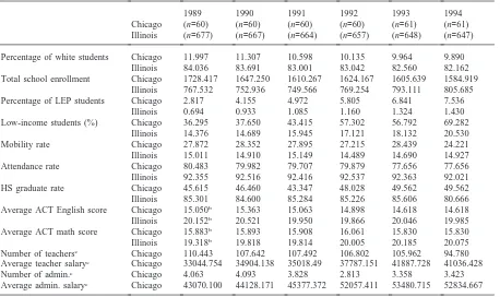
Table 1 reports means for a variety of variables for the public high schools in Chicago and for the rest of the state as a whole. Table 2 includes means and standard deviations of the variables used in our model for Chicago public high schools. The data are taken from the Illinois State Board of Education’s school report card and the
11 This data, as well as data on salaries, was provided by the Chicago Panel since the school report card only contains this information for each school district.
Table 1
Means for Chicago and Illinois high schools, 1989–1994a
1989 1990 1991 1992 1993 1994
Chicago (n=60) (n=60) (n=60) (n=60) (n=61) (n=61)
Illinois (n=677) (n=667) (n=664) (n=657) (n=648) (n=647) Percentage of white students Chicago 11.997 11.307 10.598 10.135 9.964 9.890
Illinois 84.036 83.691 83.001 83.042 82.560 82.162
Total school enrollment Chicago 1728.417 1647.250 1610.267 1624.167 1605.639 1584.919 Illinois 767.532 752.936 749.566 769.254 793.111 805.685 Percentage of LEP students Chicago 2.817 4.155 4.972 5.805 6.841 7.536
Illinois 0.694 0.933 1.085 1.160 1.324 1.430
Low-income students (%) Chicago 36.295 37.650 43.415 57.302 56.792 69.282
Illinois 14.376 14.689 15.945 17.121 18.132 20.530
Mobility rate Chicago 27.872 28.352 27.895 27.215 28.439 24.221
Illinois 15.011 14.910 15.149 14.489 14.690 14.927
Attendance rate Chicago 80.483 79.982 79.707 79.879 77.656 77.656
Illinois 92.355 92.516 92.416 92.537 92.363 92.021
HS graduate rate Chicago 45.615 46.460 43.347 48.028 49.562 49.562
Illinois 85.301 84.600 85.284 85.226 85.606 80.666
Average ACT English score Chicago 15.050b 15.363 15.063 14.898 14.618 14.618 Illinois 20.152b 20.521 19.950 19.866 20.046 19.985 Average ACT math score Chicago 15.883b 15.893 15.908 16.061 15.830 15.830 Illinois 19.318b 19.818 19.814 20.005 20.185 20.075 Number of teachersc Chicago 110.443 107.642 107.492 106.802 105.962 94.780 Average teacher salaryc Chicago 33044.754 34904.138 35018.49 37787.151 41887.728 41036.428
Number of admin.c Chicago 4.063 4.093 3.828 2.813 3.358 3.423
Average admin. salaryc Chicago 43070.100 44128.171 45377.372 52057.411 53480.715 52834.667 a Sources: Compiled by the authors using data taken from the Illinois State Board of Education, Chicago Panel on Public School Policy and Finance, and ACT (1989).
b Concordant value.
c State averages not available.
teacher and administrator data compiled from the Chicago Panel on Public School Policy and Finance. Table 1 illustrates the striking difference in character-istics between public high schools in Chicago and in the state as a whole. Chicago schools have relatively more nonwhite students, bigger enrollments, lower graduate rates, higher truancy, and lower scores. As shown in Appendix C, these differences are often statistically sig-nificant based on simple z-tests.13
Turning to Table 2 which includes descriptive stat-istics of the variables included in our model, we see that the data are fairly stable over time. In addition, standard deviations are generally smaller than the means, suggest-ing some degree of homogeneity within the sample.
13 It should be noted at this point that since the American Collegiate Test (ACT) changed its format in 1989, the scores for 1989 are not automatically comparable with those for 1990– 1994. Thus, the earlier scores for each individual school have been adjusted using a concordance table distributed by ACT; the new scores approximate those consistent with the newer “enhanced” ACT test given in recent years. A copy of the con-cordance tables appears in Appendix B .
5. Chicago high school malmquist productivity index
In this section we explicitly account for changes in the performance of Chicago high schools over time by estimating productivity change using the Malmquist pro-ductivity index described earlier.
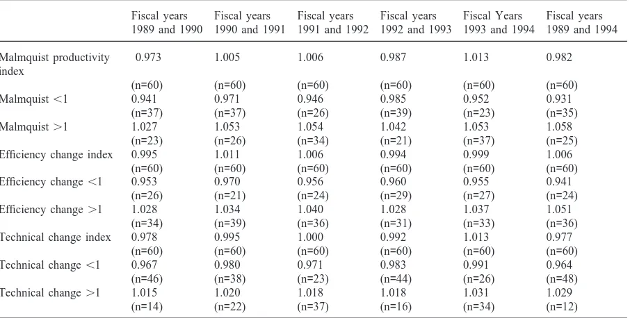
In calculating this index for Chicago high schools, only the sixty observations that appear in all six fiscal years are included. Although we estimate indexes for each high school for each pair of years, we summarize the results in Table 3. Included are the geometric means of the indirect Malmquist productivity index and all of its components, the efficiency change and the technology change indices for each pair of fiscal years. The last col-umn, which is outlined, shows the overall changes between fiscal year 1989 and 1994, averaged over the 60 schools.
pro-Table 2
Means for Chicago high school inputs and outputs, 1989–1994 (Standard deviations in parentheses)a
1989 1990 1991 1992 1993 1994
Inputs:
Number of teachers 110.443 107.642 107.492 106.802 105.962 94.780
(38.212) (35.839) (36.892) (35.838) (37.203) (31.463)
Avg. teacher salary 33044.754 34904.138 35018.149 37787.151 41887.728 41036.428 (899.388) (933.360) (1019.953) (1240.670) (1195.129) (1124.551)
Number of administrators 4.063 4.093 3.828 2.813 3.358 3.423
(1.517) (0.948) (1.048) (0.869) (1.309) (1.336)
Avg. admin. salary 43070.100 44128.171 45377.372 52057.411 53480.715 52834.667 (2526.711) (3445.006) (3368.020) (4326.771) (4115.021) (4330.407) XTEST (English ACT) 26439.294 25837.269 24845.766 24681.069 24450.248 23651.386 (12318.535) (12349.963) (12366.053) (12366.053) (12670.123) (12359.530) XTEST (Math ACT) 27788.364 26621.969 26087.068 26518.869 26170.135 25591.733
(12015.385) (12045.309) (12292.520) (12394.690) (12820.066) (12607.778) Outputs:
ATT 1405.999 1335.103 1302.979 1315.845 1283.241 1251.470
(578.836) (565.805) (579.766) (579.182) (593.876) (583.523)
HSG 823.128 791.992 740.131 818.316 805.533 819.209
(559.918) (483.784) (532.303) (562.745) (517.026) (547.751) YTEST (English ACT) 2242.069 2266.313 2202.348 2166.948 2208.623 2130.208 (2046.988) (1799.375) (1775.004) (1749.573) (1737.715) (1848.956) YTEST (Math ACT) 2352.207 2336.398 2327.326 2334.563 2371.899 2304.535
(2064.253) (1819.594) (1887.275) (1866.835) (1864.369) (1955.770) a Sources: Compiled by the authors using data taken from the Illinois State Board of Education, Chicago Panel on Public School Policy and Finance, and ACT (1989).
Table 3
Geometric means of Chicago high school Malmquist productivity index resultsa
Fiscal years Fiscal years Fiscal years Fiscal years Fiscal Years Fiscal years 1989 and 1990 1990 and 1991 1991 and 1992 1992 and 1993 1993 and 1994 1989 and 1994
Malmquist productivity 0.973 1.005 1.006 0.987 1.013 0.982
index
(n=60) (n=60) (n=60) (n=60) (n=60) (n=60)
Malmquist,1 0.941 0.971 0.946 0.985 0.952 0.931
(n=37) (n=37) (n=26) (n=39) (n=23) (n=35)
Malmquist.1 1.027 1.053 1.054 1.042 1.053 1.058
(n=23) (n=26) (n=34) (n=21) (n=37) (n=25)
Efficiency change index 0.995 1.011 1.006 0.994 0.999 1.006
(n=60) (n=60) (n=60) (n=60) (n=60) (n=60)
Efficiency change,1 0.953 0.970 0.956 0.960 0.955 0.941
(n=26) (n=21) (n=24) (n=29) (n=27) (n=24)
Efficiency change.1 1.028 1.034 1.040 1.028 1.037 1.051
(n=34) (n=39) (n=36) (n=31) (n=33) (n=36)
Technical change index 0.978 0.995 1.000 0.992 1.013 0.977
(n=60) (n=60) (n=60) (n=60) (n=60) (n=60)
Technical change,1 0.967 0.980 0.971 0.983 0.991 0.964
(n=46) (n=38) (n=23) (n=44) (n=26) (n=48)
Technical change.1 1.015 1.020 1.018 1.018 1.031 1.029
(n=14) (n=22) (n=37) (n=16) (n=34) (n=12)
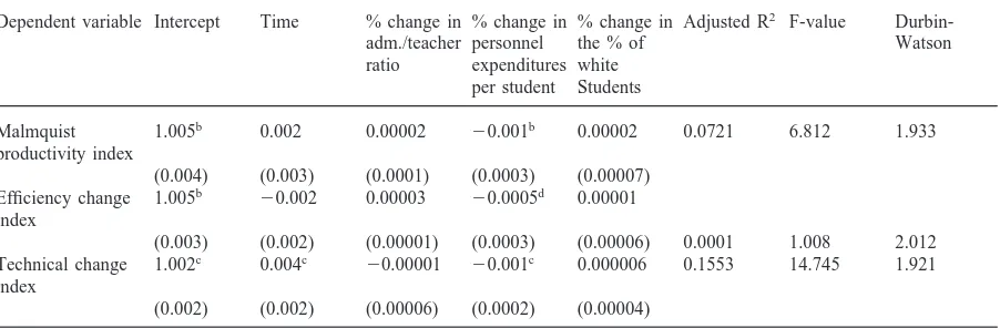
Table 4
OLS results of time trend equations for the Malmquist productivity index, 1989–1994 (Standard errors in parenthesis)a Dependent variable Intercept Time % change in % change in % change in Adjusted R2 F-value
Durbin-adm./teacher personnel the % of Watson
ratio expenditures white per student Students
Malmquist 1.005b 0.002 0.00002 20.001b 0.00002 0.0721 6.812 1.933
productivity index
(0.004) (0.003) (0.0001) (0.0003) (0.00007) Efficiency change 1.005b 20.002 0.00003 20.0005d 0.00001 index
(0.003) (0.002) (0.00001) (0.0003) (0.00006) 0.0001 1.008 2.012 Technical change 1.002c 0.004c 20.00001 20.001c 0.000006 0.1553 14.745 1.921 index
(0.002) (0.002) (0.00006) (0.0002) (0.00004)
a Sources: Compiled by the authors using data taken from the Illinois State Board of Education, Chicago Panel on Public School Policy and Finance, and ACT (1989).
b Significant at the 1 percent level of significance. c Significant at the 5 percent level of significance. d Significant at the 10 percent level of significance.
duction possibilities frontier for these schools has shifted inward slightly on average between 1989 and 1994. There is, however, a slight increase in efficiency on aver-age at the high schools. The overall averaver-age change in productivity, however, is negative.
Looking at the more disaggregated results, we see that there is a nearly even split between schools that improved in terms of productivity and those that declined. In addition, the average productivity vacillates around one on average over this time period. The same pattern occurs for the two components of productivity change. Note, however, that over half of the schools con-sistently achieve improvements in the efficiency change; i.e., they are catching up to the frontier over time.
To determine if there are any significant changes, we include a regression model in which our productivity change, technical change, and efficiency change meas-ures are dependent variables. Independent variables include a time trend, the change in the ratio of adminis-trators to teachers, the change in per pupil expenditures, and the change in the percent of students who are white. The results are summarized in Table 4.
Although we find no significant time trend in the pro-ductivity index or the efficiency change index, there is a small but significant improvement in the technical change index. The only other significant variable is the per pupil expenditure variable, which is consistently small but negative in all three regressions, i.e., schools with greater per pupil expenditure are associated with lower productivity. Finally, if we interpret the intercept term as the average value of our measures after con-trolling for our independent variables, we find that we can reject the hypothesis that the efficiency change
inter-cept is equal to one at the ten-percent level of signifi-cance, based on a simple t-test.14This suggests that there
has been a measured improvement in the efficiency of Chicago high schools on average over this time period. On the other hand, we cannot reject this hypothesis for the other index measures.
6. Concluding remarks
The purpose of this paper was to model and assess the effect of introducing site-based management to Chicago public high schools. We model the change from cen-tralized to decencen-tralized control following Grosskopf et al. (1999). This approach uses cost indirect output dis-tance functions to model decentralized control. To test for improvements over time and to determine whether these responses were brought about due to innovation or improvements in resource utilization, we compute Malmquist productivity indexes and develop these into measures of innovation (technical change or shifts in the frontier) and efficiency change. On average there was very little improvement over the 1989–94 time period. Inspection of the disaggregated results suggests that this is due to the distribution of the indexes—roughly half of
the sample achieved improvements which were offset by the half that realized declines.
A second stage regression provides some statistical evidence that there may have been a small improvement in efficiency over the 1989–94 time period. These results also suggest that schools whose per pupil expenditures were increasing over this time period had relatively lower productivity. We conjecture that these schools may have been receiving relatively more Title 1 money and have more disadvantaged students, which is broadly con-sistent with the findings by Downes & Horowitz (1994). We conclude that our evidence suggests that Chicago’s school reform experiment in site-based management resulted in mixed results in terms of performance over the 1989–94 time period.
Our results only include data on schools in the post-reform period; thus, there might have been improve-ments that we have not captured. Also, we are looking at the performance of Chicago public high schools rela-tive to themselves. If it were available, it would be extremely useful to include information on private schools and other public high schools in the state. This would allow us to compare the relative effectiveness of site-based management and magnet schools, for example.
Of course, our results lead to the obvious question— will the Daley led return to centralized control yield bet-ter performance in Chicago’s schools than site-based management achieved? Anecdotal evidence suggests that performance is improving. We would propose comp-lementing this evidence with something like the pro-ductivity indexes employed here.
Acknowledgements
We would like to thank Diane Primont of Southeast Missouri State University; Randy Dunne and Daniel Pri-mont of Southern Illinois University at Carbondale; Wil-liam W. Cooper at the University of Texas at Austin; Corrine Hansen Taylor of the University of Wisconsin at Madison and two anonymous referees for their helpful comments. In addition, this paper would not be possible without both the school report card data provided by Bill Fritcher at the Illinois State Board of Education and teacher and administrator data provided by Todd Rosen-krantz at the Chicago Panel on Public School Policy and Finance.
Appendix A. Activity analysis equations linear programming problem
In data envelopment analysis, the activity analysis model of production is used to measure efficiency and productivity. Using the notation of Grosskopf et al.
(1999), there are I observations (individual schools), M outputs, and N inputs15(of which F are fixed and N
2F
are variable); each vector of inputs and outputs is non-negative. Another important element of the activity analysis model is the inclusion of intensity variables (zi),
which describe the degree to which this activity is involved in the production process of outputs. The activity analysis linear programming problem, or DEA, used to calculate direct output distance functions for an observation i9is written as follows:
[Do(xi9f,xi9v,yi9)]−15max
The indirect output distance function can be calculated in a similar fashion using the nonparametric linear pro-gramming approach. For observation i9, we compute:
[IDo(xi9f,pi9v/ci9,yi9)]−15max
Notice that Eqs. (A.2) solves for the optimal levels of variable inputs for each school, which Eqs. (A.1) does
not. The indirect problem also includes a budget con-straint, where pv is the vector of variable input prices
and ciis the observed budget.
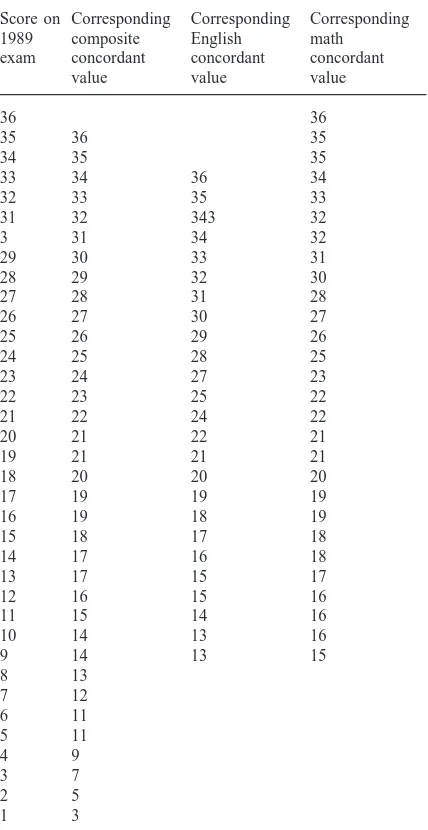
Appendix B. Adjusting 1989 ACT Scores with concordant values
When the American Collegiate Test (ACT) changed in 1989, some method of comparing the old and new scores was needed. Thus, ACT distributed Concordance Tables to make comparisons; this table appears below.
Table 5
Concordance tables for ACT exam scoresa
Score on Corresponding Corresponding Corresponding
1989 composite English math
According to ACT (1989), a concordant value “corre-sponds to the same relative standing (percent at or below) as the given score [on the old exam]”. To adjust the earlier scores so that they are consistent with the new ones, simply find the concordant value in the table on the next page corresponding to the old score. For non-whole numbers, ACT recommends rounding to the near-est whole number. This is, after all, only an approxi-mation. Table 5.
Appendix C. Chicago high school data z-statistics
Table 6.
References
ACT, 1989. The Enhanced ACT Assessment: Concordance Tables, Iowa City: American Collegiate Test, Iowa City. Aitken, M., & Longford, N. (1986). Statistical modeling issues
in school effectiveness studies. Journal of The Royal Stat-istical Society, 149A (1), 1–26.
Barrow, M. (1991). Measuring local education authority per-formance: a frontier approach. Economics of Education Review, 10, 19–27.
Bessent, A., & Bessent, W. E. (1980). Determining the com-parative efficiency of schools through data envelopment analysis. Educational Administration Quarterly, 16, 57–75. Bessent, A., Bessent, W., Kennington, J., & Reagan, B. (1982). An application of mathematical programming to assess pro-ductivity in the Houston independent school district,. Man-agement Science, 28, 1355–1367.
Boardman, A., & Murnane, R. (1979). Using panel data to improve estimates of the determinants of educational achievement. Sociology of Education, 52, 113–121. Bryk, A., Deobster, P., Easton, J., Cuppescu, S., & Thurn, Y. M.
(1994). Measuring achievement gains in the Chicago public schools. Education and Urban Society, 26, 306–319. Caves, D. W., Christensen, L. R., & Diewert, W. E. (1982). The
economic theory of index numbers and the measurement of input, output and productivity. Econometrica, 50, 1393– 1414.
Charnes, A., Cooper, W. W., & Rhodes, E. (1978). Evaluating program and managerial efficiency: an application of data envelopment analysis to program follow through. Manage-ment Science, 27, 668–696.
Chubb, J., & Moe, T. (1990). Politics, Markets and America’s Schools. Washington, DC: The Brookings Institution. Dizon, M., & Pearson, R. (1996). Edgar signs bill creating 45
charter schools, Chicago Tribune 11, (Section 1), p. 7. Downes, T.A., & Horowitz, J.L. (1994). An Analysis of the
Effect of Chicago School Reform on Student Performance. Paper presented at the Education Conference at the Federal
Reserve Bank of Chicago, Chicago.
(ftp://ftp.frbchi.org/pub/edecon94/downes.pdf)
Table 6
Hypothesis test results between variable means for Chicago high schools, 1989 and 1994 (Standard deviations in parenthesis) H0: m1989#m1994H0: m1989∃m1994OR Ha:m1989.m1994Ha:m1989,m1994a
Chicago 1989 Chicago 1994 Chicago z- Illinois 1989 Illinois 1994 Illinois
z-means means statistic means means statistic
11.997 9.890 0.828 Percentage of white students 84.036 82.162 1.165
(14.854) (13.080) (28.662) (29.793)
1728.417 1784.918 1.210 Total school enrollment 767.532 805.685 20.935
(644.812) (659.386) (742.666) (742.274)
2.817 7.536 23.214b Percentage of LEP students 0.694 1.430 23.833b
(4.312) (10.613) (2.168) (4.401)
36.295 69.282 211.555b Low-income students (%) 14.376 20.530 26.439b
(16.126) (15.255) (13.663) (20.312)
27.872 24.221 1.648 Percentage of mobile students 15.011 14.927 0.123
(13.008) (11.287) (12.669) (12.127)
80.483 77.656 2.129c Attendance rate 92.355 92.021 1.088
(6.346) (8.160) (4.976) (6.110)
45.615 49.562 21.336d HS graduation rate 85.301 80.666 4.990b
(16.835) (15.625) (16.538) (17.229)
15.050e 14.618 1.051 Average ACT English score 20.152 19.985 1.272
(2.348) (2.170) (2.423) (2.355)
15.883e 15.830 0.187 Average ACT math score 19.318 20.075 26.468b
(1.462) (1.651) (1.912) (2.156)
110.443 94.780 2.459b Number of teachersf (38.212) (31.463)
4.063 3.423 2.461b Number of adminstratorsf (1.517) (1.336)
15.608 16.404 22.120c Student/teacher ratioff (1.880) (2.232)
443.883 492.614 22.026+ Student/Admin. Ratiof (114.824) (193.576)
a Sources: Compiled by the authors using data taken from the Illinois State Board of Education, Chicago Panel on Public School Policy and Finance, and ACT (1989). Note: The hypothesis tests of ratios might not be valid if the distribution is nonnormal.
b Reject H0at 1 percent level of significance. c Reject H0at 5 percent level of significance. d Reject H0at 10 percent level of significance. e Concordant value.
f No state averages available.
schools projects in New York City and Milwaukee. Phi Delta Kappan, 64, 697–702.
Fa¨re, R., & Grosskopf, S. (1994). Cost and Revenue Con-strained Production, Bilkent University Lecture Series. Springer-Verlag.
Fa¨re, R., & Grosskopf, S. (1990). Theory and Calculation of Productivity Indexes: Revisited. Southern Illinois University at Carbondale, Economics Department Discussion Paper, Carbondale, pp. 90–98.
Fa¨re, R., Grosskopf, S., & Lovell, C. (1985). The Measurement of Efficiency of Production. Boston: Kluwer-Nijhoff. Fa¨re, R., Grosskopf, S., Lindgren, B., & Roos, P. (1989).
Pro-ductivity Development in Swedish Hospitals: A Malmquist Output Index Approach. Southern Illinois University at Car-bondale, Economics Department Discussion Paper, Carbon-dale, pp. 89–83.
Fa¨re, R., Grosskopf, S., Lindgren, B., & Roos, P. (1992). Pro-ductivity changes in Swedish pharmacies 1980–1989: a
non-parametric approach. Journal of Productivity Analysis, 3, 85–101.
Fare, R., Grosskopf, S., & Weber, W. (1989). Measuring school district performance, Public Finance Quarterly, 17, 409-428.
Fa¨re, R., Grosskopf, S., Norris, & Zhang, Z. (1994). Pro-ductivity growth, technical progress, and efficiency change in industrialized countries. American Economic Review, 84, 66-83.
Farrell, M. J. (1957). The measurement of productive efficiency. Journal of the Royal Statistical Society, 120A (3), 253–281. Garms, Guthrie, J. G., & Pierce, L. (1978). School Finance: The Economics and Politics of Public Education. Engle-wood Cliffs, NJ: Prentice-Hall, Inc.
Grosskopf, S., Hayes, K., Taylor, L., & Weber, W. (1999). Anticipating the consequences of school reform: a new use of DEA. Management Science, 45, 608–620.
Competition and School Efficiency. Paper presented at the annual meeting of the National Tax Association.
Hanushek, E.A. (1986). The economics of schooling: pro-duction and efficiency in public schools. Journal of Econ-omic Literature, 24, 1141-1177.
Hanushek, E. A., & Taylor, L. (1990). Alternative assessments of the performance of schools: measurement of state vari-ations in achievement. Journal of Human Resources, 25, 179–201.
Harp, L. (1995). Revolutionary School-Voucher Measure Falls Short in Illinois House, Education Week, 13.
Hess, G. A. Jr (1991). School Restructuring, Chicago Style. Newbury Park: Corwin Press.
Jesson, D., Mayston, D., & Smith, P. (1987). Performance assessment in the education sector: education and economic perspectives. Oxford Review of Education, 13, 249–266. Malen, B., Ogawa, R., & Kranz, J. (1990). What Do we know
about school-based management? A case study of the litera-ture—a call for research. In W. H. Clune, W. J. Witte, & J. F. Witte, Choice and Control in American Education, The Practice of Choice, decentralization and School Restructur-ing, vol. 2. London: The Falmer Press.
McCarty, T. A., & Yaisawarng, S. (1993). Technical efficiency
in New Jersey school districts. In H. O. Fried, E. Knowx-Lovell, & S. Schmidt, The Measurement of Productive Efficiency. New York: Oxford University Press.
Rogers, D., & Chung, N. H. (1983). 110 Livingston Street Revisited: Decentralization in Action. New York: New York University Press.
Rosenkranz, T. (1994). Reallocating resources: discretionary funds provide engine for change. Education and Urban Society, 26, 264–284.
Shephard, R. W. (1953). Cost and Production Functions. Prin-ceton: Princeton University Press.
Shephard, R. W. (1974). Indirect Production Functions. Mein-senhelm am Glan: Verlag Anton Hain.
Sickler, J. L. (1988a). Teachers in charge: empowering the pro-fessionals. Phi Delta Kappan, 69, 354–356.
Sickler, J. L. (1988b). Teachers in charge: empowering the pro-fessionals. Phi Delta Kappan, 69, 375–376.
Smylie, M., Crowson, R., Chou, V., & Levin, R. (1994). The principal and community-school connections in Chicago’s radical reform. Education Administration Quarterly, 30, 342–364.