Economics of Education Review 18 (1999) 405–415
www.elsevier.com/locate/econedurev
A comparison of conventional linear regression methods and
neural networks for forecasting educational spending
Bruce D. Baker
a,*, Craig E. Richards
baDepartment of Teaching and Leadership, 202 Bailey Hall, University of Kansas, Lawrence, KS 66045, USA
bDepartment of Organization and Leadership, Teachers College, Columbia University, 525 West 120th Street, Box 16, Main Hall 212A, New York, NY 10027, USA
Received 1 June 1997; accepted 2 February 1998
Abstract
This study presents an application of neural network methods for forecasting per pupil expenditures in public elemen-tary and secondary schools in the United States. Using annual historical data from 1959 through 1990, forecasts were prepared for the period from 1991 through 1995. Forecasting models included the multivariate regression model developed by the National Center for Education Statistics for their annual Projections of Education Statistics Series, and three neural architectures: (1) recurrent backpropagation; (2) Generalized Regression; and (3) Group Method of Data Handling. Forecasts were compared for accuracy against actual values for educational spending for the period. Regarding prediction accuracy, neural network results ranged from comparable to superior with respect to the NCES model. Contrary to expectations, the most successful neural network procedure yielded its results with an even simpler linear form than the NCES model. The findings suggest the potential value of neural algorithms for strengthening econometric models as well as producing accurate forecasts. [JELC45, C53, I21] 1999 Elsevier Science Ltd. All rights reserved.
Keywords:Forecasting; Time series; Neural networks
1. Introduction
From 1940 to 1990, per pupil spending on public elementary and secondary education grew from US$722 to US$4622, a constant dollar increase of 540% (Hanushek, 1994). At issue is whether educational spending as one component of our economic system is outpacing the growth and eventually the carrying capacity of the system as a whole. As a result, questions exist as to whether we can reasonably expect a continu-ance of the current rate of growth into our near or distant future. Such questions point to the increasing importance of developing and testing more sensitive forecasting methods for projecting educational expenditures.
* Corresponding author. Tel.:11-785-864-9844; fax:1 1-785-864-5076; e-mail: [email protected]
0272-7757/99/$ - see front matter1999 Elsevier Science Ltd. All rights reserved. PII: S 0 2 7 2 - 7 7 5 7 ( 9 9 ) 0 0 0 0 3 - 5
Over the past decade, neural network technologies have found their way into competitive industries from the financial markets (Lowe, 1994) to real estate (Worzala, Lenk & Silva, 1995) and health care (Buchman, Kubos, Seidler & Siegforth, 1994). Neural networks are primarily touted for their prediction accu-racy compared with conventional linear regression modeling methods. Ostensibly, neural networks are an extension of regression modeling, occasionally referred to as flexible non-linear regression (McMenamin, 1997). Recently, social scientists have begun to assess the use-fulness of neural network methods for developing a deeper understanding of trends and patterns in data, or “knowledge extraction from data,” in addition to the usual emphasis in neural network research on prediction accuracy (Liao, 1992).
gen-eral. Yet, future adoption of these methods in public fin-ance depends on our ability to establish standards for neural network application compared with conventional methods and applied to public finance forecasting prob-lems of interest. This study explores the potential value of using neural network methods alongside of more con-ventional regression methods used by the National Center for Education Statistics for forecasting edu-cational spending. A reasonable expectation, validated in other forecasting studies in public finance (Hansen & Nelson, 1997), is that neural networks, by way of flex-ible, non-linear estimation, are likely to reveal changes, or inflection points, in the general trend of education spending.
2. Neural networks
The primary objective of neural networks is predictive modeling. That is, the accurate prediction of non-sample data using models estimated to sample data. With cross-sectional data, this typically means the accurate predic-tion of outcome measures (dependent variable) of one data set generated by a given process, by providing input measures (independent variables) to a network (deterministic non-linear regression equation) trained (estimated) to a separate data set generated by the same process. With time-series data, the objective is typically forecasting, given a sample set of historical time-series realizations. This is a departure from traditional econo-metric modeling where a theoretically appropriate model is specified, then estimated using the full sample for pur-poses of hypothesis testing, the primary objective being inference.
Identification of the best predicting model begins with subdividing the sample data set into two components, the
training setand the test set, a hypothetical set of non-sample data extracted from the non-sample, against which prediction accuracy of preliminary models can be tested. Typically, thetest setconsists of up to 20% of the sam-ple (Neuroshell 2user’s manual, WSG, 1995, p. 101). For time-series modeling, thetest setconsists of the most recent realizations. The objective is to identify the model which, when estimated to the training set, most accu-rately predicts the outcome measures of the test set as measured by absolute error or prediction squared error. It is then expected that the same model will best predict non-sample data, sometimes referred to as theproduction set(WSG, 1995, p. 101).
Two methods are typically used for estimating the deterministic neural network model: (1) iterative conver-gent algorithms and (2) genetic algorithms. Superficially, the iterative, convergent method begins by randomly applying a matrix of coefficients (connection weights) to the relationships from each independent variable to the dependent variable of the training set. The weights are
then used to predict the outcome measure of the test set. Prediction error is assessed, and either a new set of ran-dom weights is generated, or learning rate and momen-tum terms dictate the network to incrementally adjust the weights based on the direction of the error term from the previous iteration (WSG, 1995, pp. 8, 52, 119). The pro-cess continues until several iterations pass without further improvement of test set error. The genetic algor-ithm approach begins by randomly generating pools of equations. Again superficially explained, initial equa-tions are estimated to the training set and prediction accuracy of the outcome measure is assessed using the test set to identify a pool of the “most fit” equations. These equations are then hybridized or randomly recom-bined to create the next generation of equations. That is, parameters from the surviving population of equations may be combined, or excluded to form new equations as if they were genetic traits. This process, like the iterative, convergent application of weights, continues until no further improvement in predicting the outcome measure of the test set can be achieved.
A common concern regarding flexible non-linear mod-els is the tendency to “overfit” sample data (Murphy, Fogler & Koehler, 1994). It has been shown, however, that while iterative or genetic, selective methods can gen-erate complex non-linear equations that asymptotically fit the training set, the prediction error curve with respect to non-linear complexity for the test set isU (Murphy et al, 1994) orV(Farlow, 1984) shaped; that is, beyond an identifiable point, additional complexity erodes, rather than improves, prediction accuracy of the test set.
Backpropagation algorithms are among the oldest, and until recently, most popular neural networks (Caudill, 1995, p. 5). Backpropagation primarily describes an esti-mation procedure. Apply the previously discussed iterat-ive estimation method to the regression equation
Y5b1X11e
Iterative estimation of the equation involves selecting the initial value forbat random, evaluating the predic-tion error ofY, and incrementally adjusting buntil we have reduced prediction error to the greatest extent poss-ible. This description represents a “single output, feed forward system with no hidden layer and with a linear activation function” (McMenamin, 1997, p. 17). The typical backpropagation neural network consists of three layers, and can be represented in regression terms as
Y5F[H1(X),H2(X),…,HN(X)]1e
same applies for all Xs. While for inferential purposes this replication results in irresolvable collinearities, in the three-layer backpropagation network it allows for alter-nate weighting schemes to be applied to the same inputs, creating the possibility of different sensitivities of the outcome measure at different levels of each input, resulting in heightened prediction accuracy. The resca-ling procedure, activation function or “hidden layer transfer function” (McMenamin, 1997), sometimes referred to as squashing (Rao & Rao, 1993), typically involves rescaling all inputs to a sigmoid distribution using either a logistic or hyperbolic tangent function. Backpropagation has proven an effective tool for both time-series prediction (Hansen & Nelson, 1997; Lachter-macher & Fuller, 1995) and cross-sectional prediction (Buchman et al, 1994; Odom & Sharda, 1994; Worzala et al, 1995).
Two alternatives used in addition to backpropagation in this study are (1) Generalized Regression neural net-works (GRNN) (Specht, 1991) and (2) Group Method of Data Handling (GMDH) polynomial neural networks (Farlow, 1984). Both involve identifying best predicting non-linear regression models. An advantage of Specht’s GRNN is removal of the necessity to specify a functional form by using the observed probability density function (pdf) of the data (Caudill, 1995, p. 47). GRNN interp-olates the relationship between inputs, and inputs and outcomes by applying smoothing parameters (a) to mod-erate the degree of non-linearity in the relationships and serve as a sensitivity measure of the non-linear response of the outcome to changes in the inputs. Smoothing para-meters typically vary among model inputs with the opti-mal combination of smoothing parameters being selected by (1) a holdout method1 or (2) a genetic adaptive
method.2GRNN has been implicated for effective
cross-sectional prediction of binary outcomes (Buchman et al, 1994) and recommended for time-series prediction, parti-cularly for use with sparse data and data widely varying in scale (Caudill, 1995, p. 47).
A.G. Ivakhnenko (1966, in Farlow, 1984) proposed GMDH for identifying a best prediction polynomial via a Kolmogorov–Gabor specification.3GMDH polynomial
fitting differs from backpropagation and GRNN in that
1Described by Specht (1991) but not used in this study. Thus due to space constraints we opt not to discuss this method furth-er.
2Recommended for identifying best predicting models where “input variables are of different types and some may have more of an impact on predicting the output than others” using Neuro-shell 2(WSG, 1995, p. 138).
am) is the vector of coefficients or weights (Liao, 1992).
no training set is specified. Rather a measure referred to as FCPSE (Full Complexity Prediction Squared Error) is used. FCPSE consists of a combination of Training Squared Error4 combined with an overfitting penalty
similar to that used for the PSE (Prediction Squared Error)5 but including additional penalty measures for
model complexity.6 Also unlike backpropagation,
GMDH generally applies linear scaling to inputs.7
3. Methods
3.1. Data
All data used for this study were provided by the National Center for Education Statistics (NCES) (see Appendix A). Complete annual time series for all vari-ables in the models were available from 1959 through 1995. Variables used in the analyses include:
CUREXP: Current expenditures per pupil in average daily attendance
PCI: Per capita income
ADAPOP: Ratio of average daily attendance to the population
SGRNT: Local governments’ education receipts from state sources per capita
BUSTAX: Business taxes and non-tax receipts to state and local governments per capita
PERTAX: Personal taxes and non-tax receipts to state and local governments per capita
RCPIANN: Inflation rate measured by the consumer price index
All variables are measured in 1982–84 constant dol-lars.8
While actual data were available for use as predictors for 1991 through 1995, the intent of this study was to mimic true forecasting circumstances, where such values would not be available, thus necessitating univariate
4Referred to as Norm.MSE. Discussed in more detail in WSG (1995) pp. 149–151.
5PSE5 Norm.MSE1 23 var(p)3 k/N, whereNis the number of patterns in the pattern file, andkis the number of coefficients in the model (which are determined in order to min-imize Norm.MSE) (WSG, 1995, p. 149).
6WSG retains proprietary rights to the design of FCPSE and therefore does not disclose the formula for its determination (WSG, 1995, p. 150).
7X9 523(X2Min)/((Max2Min)21), further described in WSG (1995, p. 158).
forecasts of predictors. For all univariate analyses mod-els were estimated to data from 1959 through 1990 and forecasts generated from 1991 through 1995. For all multivariate models, equations were estimated, or neural networks trained, on time series from 19609 through
1990 and forecasts generated from 1991 through 1995. Forecasts (1991–1995) were compared for accuracy with actual values for Current Expenditures per Pupil reported by NCES.
3.2. Univariate models and forecasts
Univariate models were estimated for all series using the SAS System (v6.12) selection procedure, which applies a variety of trend analyses, exponential smoo-thing methods and ARIMA models to untreated, logged and differenced forms of each series. Forecasting models were selected for each series on the basis of Root Mean Square Error (RMSE).
3.3. The multivariate (AR1) regression model
The multivariate regression model used for forecasting educational spending is based on the National Center for Education Statistics models annually published in the Projections of Education Statistics series (Gerald & Hus-sar, 1996–1998). The model consists of two multiple regression equations that have taken various forms over the years. The model is based on a median voter model which presumes that spending for public goods reflects the preferences of the median voter; that is, the voter in the community with the median income and/or median property value. In recent years, both equations in the model have assumed a multiplicative functional form, thus requiring the use of the natural log form of all ser-ies. Estimation of the model equations has typically been performed using AR1 methods in order to correct for autocorrelation of residuals.10
The primary equation for forecasting Current Expendi-tures per Pupil can be expressed:
ln CUREXP5b01b1ln PCI1b2ln SGRNT (1)
1b3ln ADAPOP1u
where CUREXP, PCI, SGRNT and ADAPOP are as pre-viously defined, (ln) refers to the natural logarithm and “u” is the error term expected to display first-order auto-correlation.
The model requires a secondary equation for
generat-9While data were available back to 1959, accommodation of lagged variables reduced the estimable series by one period.
10For a more in-depth discussion of the theoretical basis and mathematical specification of the model, consult Gerald and Hussar (1996–1998, pp. 151–154).
ing forecast predictors of SGRNT, the measure of state contributions. The equation takes the following form: ln SGRNT5b01b1ln BUSTAX{1}
1b2ln PERTAX{1}1b3ln ADAPOP (2)
1b4ln (RCPIANN/RCPIANN{1})1u
where BUSTAX,11PERTAX, ADAPOP and RCPIANN
are as previously defined, {1} refers to a lag of one per-iod and “u” is the error term expected to display first-order autocorrelation. AR1 estimation of the model was conducted using RATS 4.0 (Regression Analysis of Time Series, 32-bit version).12 Forecasts of ln SGRNT
and ln CUREXP were also prepared in RATS applying the respective equations. Updating of coefficient esti-mates was not used.
3.4. Neural network methods
All neural networks were estimated (trained) and fore-casts prepared usingNeuroshell 2 (Release 3.0, 32-bit) (WSG, 1995). For backpropagation, a Jordan–Elman recurrent backpropagation architecture, where the net-work includes a connection from the output layer to the input layer, was selected.13 Caudill (1995, pp. 19–24)
recommends recurrent backpropagation for time-series prediction. Default learning parameters were applied.14
For the Generalized Regression neural networks (GRNN), the genetic adaptive algorithm was used for smoothing parameter selection. Most default parameters
11BUSTAX is not included in Gerald and Hussar’s most recent (1997) models, but was included in earlier iterations (1996). We have chosen to include this variable for two reasons: (1) our re-estimates of the NCES models, the effects of includ-ing this variable on forecast accuracy are negligible; and (2) we wished to include this variable in the training procedures of the neural network algorithms in order to allow the neural network to determine, for itself, the value of the additional predictor. Therefore, inclusion in the conventional model was for the pri-mary purpose of retaining comparability.
12For more detail on the RATS AR1 procedure see RATS user’s manual (Doan, 1996, pp. 5–6, 14–6).
13The particular importance of the output–input connection is discussed in WSG (1995, pp. 106–107).
were applied.15 For Group Method of Data Handling
(GMDH), default parameters were also applied.16
For both the recurrent backpropagation models and Generalized Regression neural networks, the training sets consisted of data from 1960 to 1980 and test sets consisted of data from 1981 through 1990.17 Alternate
models were trained with log (ln) transformed data. Pre-dictors and lags were the same as those specified for the linear regression equation. Only the main equation for the prediction of CUREXP was modeled with the neural networks. Forecasts were generated for the period from 1991 through 1995 by providing the trained neural net-works with the same set of forecast predictors (univariate results) used for the linear regression model including regression predictions of SGRNT from the secondary multiple linear regression equation.
4. Results and discussion
4.1. Univariate models
All models selected for univariate forecasting were either (1) Linear (Holt) Exponential Smoothing18(PCI,
PERTAX) or (2) Damped Trend Exponential Smoothing (ADAPOP, BUSTAX, RCPIANN) models. Parameters for the models and measures of fit are displayed in Appendix B.
4.2. Multivariate model
The estimated AR1 multivariate regression model for forecasting SGRNT is:
ln SGRNT50.13 (0.90)
15Including linear scaling (0,1) of the input layer and model selection based on test set error, with the stop criterion set to 20 generations without reduction of error. One alteration made was increasing the size of the gene pool to 300 from the default of 20. Incrementally increased gene pool size, while requiring longer training times, produced more accurate results.
16Including linear scaling of the input, 21,11 > > and output layers [21,11], “Smart” model selection and optimiz-ation, applying FCPSE as the selection criteria, and the option to construct a model of “high” non-linearity, indicating the option to include second- and third-order terms on all para-meters and two- and three-way interactions.
17An arbitrary specification of 33%, in excess of the rec-ommended 20% (WSG, 1995, p. 101) test set that yielded equi-valent results.
18Which for prediction or forecasting purposes can be expressed as: Zˆn(l) 5 a[Zn 1 (12a)Zn21 1 (12
a)2Z
n221…]5 Sn, where the predicted future observation
Zˆn(l) is based on previous observations Zn−t multiplied by a
decaying smoothing constanta, (12a)2… andS
nrepresents
the smoothed statistic (Liu & Hudak, 1994, p. 9.3).
10.67 ln BUSTAX{1} (0.04)
10.30 ln PERTAX{1} (0.12) (3)
10.31 ln ADAPOP (0.01)
20.03 ln(RCPIANN/RCPIANN{1}) (0.08)
with Rho50.19 (0.37),R250.992,p-values in
parenth-eses.
Forecasts of SGRNT were generated from this model using the univariate forecasts of predictors (BUSTAX, PERTAX, ADAPOP, RCPIANN) (Appendix C).
The estimated AR1 multivariate regression model for forecasting CUREXP is:
ln CUREXP5 21.30 (0.29)
10.55 ln PCI (0.02)10.63 ln SGRNT (0.00) (4)
20.32 ln ADAPOP (0.02)
with Rho50.41 (0.04),R250.997,p-values in
parenth-eses.
Forecasts of CUREXP were generated from this model using the univariate forecasts of PCI and ADAPOP, and multivariate forecast of SGRNT (Appendix C).
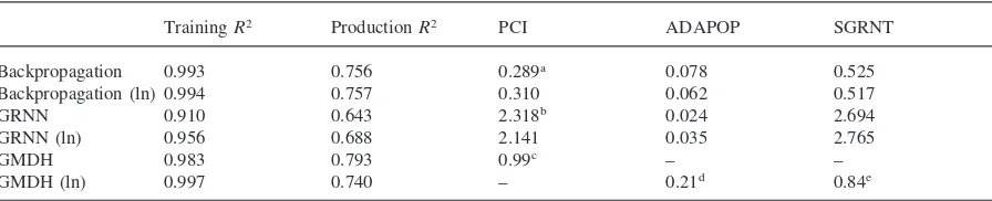
4.3. Neural models
Table 1 displays the training (sample fit) and pro-duction (forecast fit) results for each of the neural net-work models, including both fitness measures and each network’s respective measure of input contribution to prediction. For the recurrent backpropagation models, each obtained exceptionally strong fit to the training set (R250.993 to 0.994(ln)) and produced reasonable fit to
the production set (R250.756 to 0.757(ln)). The
aggre-gate contribution factors19 implicate state-level support
(SGRNT) as the primary influence on spending. Both GRNN models were slightly less fit (R250.910
to 0.956(ln)) to the training set than recurrent backpagation models and both produced looser fit to the pro-duction set (0.643 to 0.688(ln)). Again, aggregate weighting factors, in this case smoothing parameters, suggest relatively high importance of state-level support (SGRNT) for predicting spending (CUREXP).
GMDH produces comparable fitness to both training and production sets to recurrent backpropagation. Note,
Table 1
Training and forecast fitness of neural models
TrainingR2 ProductionR2 PCI ADAPOP SGRNT
Backpropagation 0.993 0.756 0.289a 0.078 0.525
Backpropagation (ln) 0.994 0.757 0.310 0.062 0.517
GRNN 0.910 0.643 2.318b 0.024 2.694
GRNN (ln) 0.956 0.688 2.141 0.035 2.765
GMDH 0.983 0.793 0.99c – –
GMDH (ln) 0.997 0.740 – 0.21d 0.84e
PCI: per capita income; ADAPOP: average daily attendance as a percent of the population; SGRNT: state-level support to public education (per pupil in ADA)
aAggregate weighting or “Contribution” factor (see WSG, 1995, p. 191). bAggregate smoothing factor (a) (see WSG, 1995, pp. 198–205).
cLinear coefficient (b), based on rescaled PCI (ˆPCI)523(PCI27504.39)/13932.6121. dLinear coefficient (b), based on rescaled SGRNT (ˆSGRNT)523(ln SGRNT24.79)/1.2821. eLinear coefficient (b), based on rescaled ADAPOP (ˆADAPOP)523(ln ADAPOP11.98)/0.4821.
however, that the GMDH model that produces greater fit to the training data (0.997(ln) compared to 0.983) does not perform as well on the production data (0.740(ln) compared to 0.793). In addition, while measures of pre-dictor importance were fairly consistent between back-propagation and GRNN models, GMDH models took varied forms, with the first (not log transformed) includ-ing only per capita income and the second (log transformed) including only state support and average daily attendance. Interestingly, though GMDH learning was set for the possibility of including both second- and third-order terms as well as two- and three-way interac-tion terms, resultant (best predicting) models included only first-order (linear) parameters.
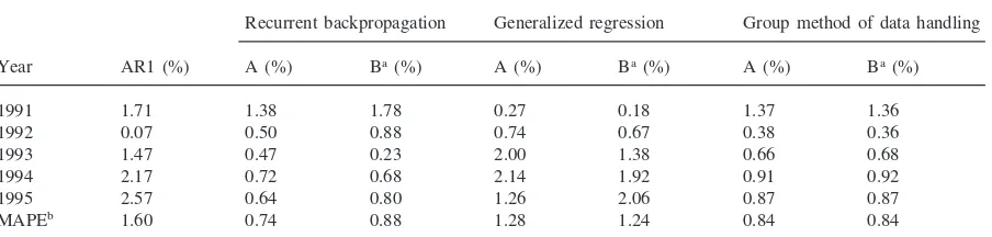
4.4. Model forecasts and accuracy assessment
Table 2 displays the AR1 and neural forecasts of edu-cational spending alongside actual spending values (1982–1984 constant dollars) for the period 1991–1995. Note that beyond 1993 all models provide overestimates
Table 2
Comparison of forecast accuracy
Group method of data Recurrent backpropagation Generalized regression
handling
Year Actual (US$) AR1 (US$) A (US$) Ba(US$) A (US$) Ba(US$) A (US$) Ba(US$)
1991 3923 3856 3869 3853 3934 3917 3870 3870
1992 3920 3918 3901 3886 3949 3947 3906 3906
1993 3916 3973 3934 3925 3994 3970 3942 3942
1994 3942 4027 3970 3968 4026 4017 3977 3978
1995 3979 4081 4004 4010 4029 4061 4013 4013
Prices reported in constant school-year 1982–84 dollar using reported consumer price index (CPI) as the deflator. aIndicates model trained with log (ln) transformed series.
of educational spending, the most significant overesti-mates coming from the AR1 model.
Table 3 displays the comparisons of forecast accuracy for the AR1 multiple regression model and the three neu-ral network models. While the NCES model performed quite well for the entire period (MAPE51.60%), each of the neural models outperformed the NCES model on average for the forecast period. Period-to-period predic-tions, however, vary quite significantly, for example, with the AR1 model outperforming the others for the second (1992) time period. Overall, recurrent backpro-pagation and GMDH models performed particularly well, providing an approximate 23increase in forecast accuracy over the NCES model.
aver-Table 3
Comparison of forecast accuracy
Recurrent backpropagation Generalized regression Group method of data handling
Year AR1 (%) A (%) Ba(%) A (%) Ba(%) A (%) Ba(%)
1991 1.71 1.38 1.78 0.27 0.18 1.37 1.36
1992 0.07 0.50 0.88 0.74 0.67 0.38 0.36
1993 1.47 0.47 0.23 2.00 1.38 0.66 0.68
1994 2.17 0.72 0.68 2.14 1.92 0.91 0.92
1995 2.57 0.64 0.80 1.26 2.06 0.87 0.87
MAPEb 1.60 0.74 0.88 1.28 1.24 0.84 0.84
aIndicates model trained with log (ln) transformed series.
bAmong others, Chase (1995) explains the interpretation and use of Mean Absolute Percentage Error (MAPE) in assessing forecast accuracy.
age backpropagation and GMDH forecasts increased (0.9%). GRNN forecasts increased more slowly (from 0.7% to 0.8%), with a low of 0.4% for 1991–1992 (GRNN) and 0.6% for 1992–1993 (ln GRNN). That GRNNs revealed this pattern is consistent with Caudill’s (Caudill, 1995, pp. 47–48) suggestion that GRNNs are particularly sensitive to non-linear relationships in sparse and/or noisy data.
5. Conclusions and recommendations
Neural network algorithms display promise for use in multivariate forecasting, although not necessarily for the expected reasons. It was presumed at the outset of this study that the primary advantage of neural networks would be their ability to flexibly accommodate non-lin-ear relationships among variables. Non-linnon-lin-ear functions were expected to better represent the changing relation-ships between economic indicators over time, thus pro-ducing more accurate, more sensitive forecasts. Contrary to our expectations, two of the best performing models, the GMDH models of both the standard and log transfor-med series, generated by neural network algorithms con-tained only linear parameters. That non-linear estimation
seemed not to advantage neural networks in this study is likely a result of the relatively high linearity of the nationally aggregated annual measures used.
Appendix A
Data for model estimation
Year CUREXP PCI SGRNT ADAPOP PERTAX RCPIANN BUSTAX CPI 1959 1205 8,624 97 0.178 84 1.371 274 0.290 1960 1292 8,744 110 0.183 95 1.438 291 0.294 1961 1322 8,757 113 0.185 100 1.248 301 0.298 1962 1413 9,063 123 0.189 108 1.036 319 0.301 1963 1424 9,243 130 0.193 115 1.220 322 0.304 1964 1492 9,605 138 0.198 122 1.424 344 0.309 1965 1547 10,102 145 0.200 132 1.296 362 0.313 1966 1684 10,645 160 0.202 139 2.159 390 0.319 1967 1740 10,982 165 0.203 157 3.105 400 0.329 1968 1935 11,335 182 0.205 170 3.341 427 0.340 1969 1939 11,615 194 0.206 194 4.874 456 0.357 1970 2159 11,985 210 0.207 212 5.908 477 0.378 1971 2294 12,293 214 0.207 214 5.094 492 0.397 1972 2407 12,548 224 0.203 252 3.630 532 0.412 1973 2515 13,323 230 0.201 281 4.029 564 0.428 1974 2588 13,607 244 0.196 274 8.953 561 0.467 1975 2635 13,392 244 0.194 267 11.022 544 0.518 1976 2711 13,707 264 0.191 278 7.080 551 0.555 1977 2789 14,007 254 0.187 300 5.875 571 0.587 1978 2910 14,539 254 0.182 316 6.670 584 0.626 1979 2949 14,971 263 0.176 314 9.393 588 0.685 1980 2927 14,988 260 0.170 306 13.281 565 0.776 1981 2888 15,014 254 0.166 303 11.606 556 0.866 1982 2895 15,172 242 0.161 304 8.687 545 0.942 1983 3010 15,171 247 0.158 314 4.275 557 0.982 1984 3117 15,898 253 0.155 346 3.701 604 1.018 1985 3280 16,628 269 0.154 362 3.921 633 1.058 1986 3449 16,930 284 0.153 374 2.906 662 1.089 1987 3567 17,143 294 0.153 404 2.235 672 1.113 1988 3657 17,528 298 0.153 403 4.155 682 1.159 1989 3831 17,883 309 0.152 419 4.572 684 1.212 1990 3920 18,042 313 0.153 431 4.784 686 1.270
Source: National Center for Education Statistics (1998). Variable definitions on page 3.
Appendix B
Univariate model estimates
Parameters for univariate models
Linear (Holt) exponential smoothing models
LEVEL wgta TREND wgtb
Variable Smoothed level Smoothed trend RMSE R2
(p-value) (p-value)
PCI 0.999 (0.0001) 0.001 (0.9772) 180.42 311.82 214.96 0.995 PERTAX 0.999 (0.0001) 0.001 (0.9886) 430.77 11.13 11.29 0.988
aWhere the level weight,a, is used in the determination of the calculated averageZ
tby the equationZt5a(Zt)1
(12a)Zt21(Armstrong, 1985, p. 165).
bWhere the trend weight, b, is used in the determination of the calculated trend by the equation G
t5b(Zt2 Zt21)1(12b)(Gt21) (Armstrong, 1985, p. 168).
Damped trend exponential smoothing models
LEVEL wgt TREND wgt Smoothed Smoothed
Variable DAMPING wgta RMSE R2
(p-value) (p-value) level trend
ADAPOP 0.868 (0.0001) 0.999 (0.0125) 0.917 (0.0001) 0.153 0.0005 0.001 0.995 BUSTAX 0.999 (0.0005) 0.999 (0.2278) 0.713 (0.0004) 685.69 1.959 14.33 0.987 RCPIANN 0.999 (0.0001) 0.001 (0.9914) 0.990 (0.0001) 4.78 0.08 1.88 0.662
aWhere the damping factor (0, K
Appendix C
Base forecasts of SGRNT
Forecasts of predictors for SGRNT equation
BUSTAX{1}a PERTAX{1}b RCPIANN{1}e
Year ADAPOPc (US$) RCPIANNd(US$)
(US$) (US$) (US$)
1991 685 430 0.153 4.861 4.649
1992 687 442 0.154 4.936 4.861
1993 688 453 0.154 5.012 4.936
1994 689 464 0.154 5.086 5.012
1995 689 475 0.155 5.159 5.086
aBusiness tax receipts lagged one period. bPersonal tax receipts lagged one period.
cAverage daily attendance as a percent of the population. dInflation rate (change in CPI).
eInflation rate lagged one period.
Forecasts of predictors for main equation
Year PCIa(US$) ADAPOPb SGRNTc (US$)
1991 18,354 0.153 311
1992 18,666 0.154 315
1993 18,978 0.154 318
1994 19,289 0.154 320
1995 19,601 0.155 323
aPer capita income.
bAverage daily attendance as a percent of the population. cState level support to public education (per pupil in ADA).
References
Armstrong, J.S. (1985).Long-range forecasting: From crystal ball to computer. New York: Wiley.
Buchman, T.G., Kubos, K.L., Seidler, A.J., & Siegforth, M.J. (1994). A comparison of statistical and connectionist models for the prediction of chronicity in a surgical intensive care unit.Journal of Critical Care Medicine,22(5), 750–762. Caudill, M. (Ed.) (1995). Using neural networks. AI Expert
(Special Issue), February.
Chase, C.W. (1995). Editorial: Measuring forecast accuracy. Journal of Business Forecasting,14(3), 2.
Doan, T. (1996). RATS (regression analysis of time series) user’s guide. Evanston, IL: Estima Products.
Farlow, S.J. (1984). Self-organizing method of modeling: GMDH type algorithms. New York: Marcel Dekker.
Gerald, D., & Hussar, W. (1996–1998). Projections of edu-cation statistics to 2006. Washington, DC: National Center For Education Statistics, US Department of Education. Hansen, J.V., & Nelson, R.D. (1997). Neural networks and
tra-ditional time-series methods: a synergistic combination in state economic forecasts.IEEE Transactions on Neural Net-works,8(4), 863–873.
Hanushek, E. (1994). Making schools work: Improving per-formance and controlling costs. Washington, DC: Brook-ings Institution.
Lachtermacher, G., & Fuller, D. (1995). Backpropagation in time-series forecasting. Journal of Forecasting, 14(4), 381–393.
Liu, L.M., & Hudak, G.B. (1994).Forecasting and time series analysis using the SCA statistical system. Chicago, IL: Scientific Computing Associates.
Lowe, D. (1994). Novel exploitation of neural network methods in financial markets.IEEE Transactions on Neural Networks 3623–3628.
McMenamin, J.S. (1997). A primer on neural networks for fore-casting.Journal of Business Forecasting,16(3), 17–22. Murphy, C., Fogler, H.R., & Koehler, G. (1994). Artificial
stu-pidity.ICFA Continuing Education30 March, 44–49. Odom, M., & Sharda, R. (1994). A neural network model for
bankruptcy prediction. Unpublished manuscript, Oklahoma State University.
Rao, V., & Rao, H. (1993).C1 1neural networks and fuzzy logic. New York: MIS Press.
Specht, D.F. (1991). A generalized regression neural network. IEEE Transactions on Neural Networks,2(5), 568–576. Ward Systems Group (WSG). 1995. Neuroshell 2. User’s
Guide. Frederick, MD: WSG.