EVALUATING THE NOVEL METHODS ON SPECIES DISTRIBUTION MODELING
IN COMPLEX FOREST
C. H. Tua, N. J. Lob, W. I Changc, K. Y. Huangd, *
a
Graduate student, Dept. of Forestry, Chung-Hsing University, Taiwan, E-mail: [email protected] b
Specialist, EPMO, Chung-Hsing University, Taiwan, E-mail: [email protected] c
Director, Hsinchu Forest District Office, Taiwan, E-mail: [email protected] d
Professor, Dept. of Forestry, Chung-Hsing University, Taiwan, E-mail: [email protected] 250 Kuo-Kuang Road, Taichung 402, Taiwa, R. O. C.
Commission II, WG II/3 KEY WORDS: Ecology, Forestry, GIS, Prediction, Statistics, Modelling
ABSTRACT:
The prediction of species distribution has become a focus in ecology. For predicting a result more effectively and accurately, some novel methods have been proposed recently, like support vector machine (SVM) and maximum entropy (MAXENT). However, high complexity in the forest, like that in Taiwan, will make the modeling become even harder. In this study, we aim to explore which method is more applicable to species distribution modeling in the complex forest. Castanopsis carlesii (long-leaf chinkapin, LLC), growing widely in Taiwan, was chosen as the target species because its seeds are an important food source for animals. We overlaid the tree samples on the layers of altitude, slope, aspect, terrain position, and vegetation index derived from SOPT-5 images, and developed three models, MAXENT, SVM, and decision tree (DT), to predict the potential habitat of LLCs. We evaluated these models by two sets of independent samples in different site and the effect on the complexity of forest by changing the background sample size (BSZ). In the forest with low complex (small BSZ), the accuracies of SVM (kappa = 0.87) and DT (0.86) models were slightly higher than that of MAXENT (0.84). In the more complex situation (large BSZ), MAXENT kept high kappa value (0.85), whereas SVM (0.61) and DT (0.57) models dropped significantly due to limiting the habitat close to samples. Therefore, MAXENT
model was more applicable to predict species’ potential habitat in the complex forest; whereas SVM and DT models would tend to underestimate the potential habitat of LLCs.
* Corresponding author.
1. INTRODUCTION
Recently, the prediction of species’ distribution and potential
habitat has been implemented widely and become a focus in ecology (Miller et al., 2004). With the innovations of remote sensing (RS) and geographic information system (GIS) tools and statistical techniques, the predictive capability of models is substantially increasing and the models can be used to classify the dataset in more detail, like the classification of similar tree species (Dalponte et al., 2008).
Most of the previous studies were located in large areas of pure
or planted forest or agricultural area to predict plant’s
present/absence or health and growth conditions. Few of them were devoted to classify the species in a complex forest, like the forests in Taiwan. Many species in a complex forest have the biophysiological characteristics so similar that they are difficult to discriminate. The complexity in forest with high biodiversity will cause more interaction among species. Furthermore, the competition among species will result in that a species might be absence in its suitable habitat so that hard to predict precisely. To classify the species accurately, we must consider about the elements in modeling, including predictive variables, quality of data, statistical methods, and so on (Guisan and Zimmermann, 2000). In terms of statistical methods, each method was developed from different principles on each scientific field, like entropy, regression, or envelope, and they will generate different results that can be used in different applications, like economic, demography, or ecology, or different level, like different scale.
Support vector machine (SVM) is a novel method that has been used widely for classification and identification studies (Dalponte et al., 2008; Drake et al., 2006; Guo et al, 2005; Melgani and Bruzzone, 2004). Maximum entropy (MAXENT) is also a novel method, and it has been demonstrated for predictive research in ecology (Elith et al., 2006; Hernandez et al., 2006; Kumar and Stohlgren, 2009; Peterson et al., 2007). These two methods were chosen to build the predictive models in this study, and comparing with a classification techniques, decision tree (DT) that are commonly used in most investigations (Bourg et al., 2005; De’ath and Fabricius, 2000; Felicísimo and Gómez-Muñoz, 2004; Landenburger et al., 2008;
and O’Brien et al., 2005) to evaluate the capability for
predicting the potential habitat.
Castanopsis carlesii (Long-leaf chinkapin, LLC) trees grow widespread in the mountains in central Taiwan and are an important heliophilous species. According to the field survey in the past, this species may only grow above the elevation of 1700 m. Seeds of LLCs have long been recognized as an important food source for animals, showing that their value of ecological system has been significant.
In this study, we aim to evaluate which method will be the most applicable for the prediction of species’ potential habitat in the complex forest. We used a GIS to overlay field tree samples on environmental layers of altitude, slope, aspect, terrain position, and vegetation indices derived from SPOT-5 images to analyze the distribution of LLCs. The complexity in forest (biodiversity) where single species will live in smaller area with the increasing of biodiversity was represented by large background sample
size. Three methods, SVM, MAXENT, and DT, were chosen to establish the predictive models.
2. STUDY AREA
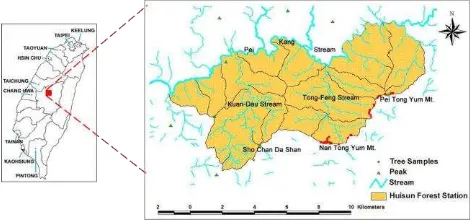
The study area encompasses the Huisun Experimental Forest Station, the property of National Chung-Hsing University, situated within 242´–245´ N latitude and 121´–1217´ E longitude, in central Taiwan. The station has a total area of 7, 477 ha. Its elevation ranges from 454 m to 2, 419 m, and its climate is temperate and humid. Hence, the study area has nourished many different plant species (more than 1100 species) and is a representative forest in central Taiwan. It comprises five watersheds, including two larger watersheds, Kuan-Dau at west and Tong-Feng at east (Figure 1).
Figure 1. Location map of the study area
3. METHODS AND MATERIAL 3.1 Data Collection and Processing
3.1.1 Field Data: LLC samples were acquired from the study area by using a GPS linked with a laser range. The error of the system would be below one meter after post differential positioning, and the sample data were rectified to the TWD67 (GRS67) Transverse Mercator map projection of two-degree zone. Total number of LLC samples we acquired was 123. There were 105 LLC samples acquired from Tong-Feng watershed, where two-third of them (72) were used to establish predictive models (Training Set), and one-third of them (33) were used in model validation (Test Set 1). Remaining 18 tree samples were from the sites with 0.5 km gap from the west side of Tong-Feng watershed, and were used to examine the ability of extrapolating of models (Test Set 2).
Because background sites (non-target) correspond to the vast majority of the study area, larger variation is expected in environmental characteristics for this group. The number of background pixels (sites) should be three times more than that of target pixels to acquire a more representative sample of the habitat characteristics at background sites (Pereira and Itami, 1991; Sperduto and Congalton, 1996), and the background sample data were taken from data layers by random sampling technique (pseudo-absence) to minimize spatial autocorrelation in the independent variables (Pereira and Itami, 1991).
The proportion of relative occurrence area of single species will decrease with increasing of the biodiversity in the forest due to the competition among species, and thus we raised the background sample size to stand for the higher biodiversity in the forest. In Training Set, we took the background sample size about five times and 100 times more than target sample size to represent low biodiversity (LB) and high (HB) biodiversity,
respectively. In Test Sets 1 and 2, we only used five times background sample size to test both two types of models.
3.1.2 Digital Elevation Model: Digital elevation model (DEM) was acquired from the Aerial Survey Office, Forestry Bureau of the Council of Agriculture, Taiwan. To meet the requirements of the study, the DEM was interpolated into 5 5 m grid size, geo-referenced to the coordinate system, TWD67 (Taiwan Datum spheroid: GRS67) and Transverse Mercator map projection over two-degree zone with the central meridian 121E.
The altitude data layer was derived directly from the DEM. Slope and aspect data layers were generated from the DEM by using ERDAS Imagine software.
3.1.3 Orthophoto Base Maps: We used orthophoto base maps (1:10,000) together with DEM to generate terrain position layer. We calculated the Euclidean distance from each pixel to the nearest ridge and the nearest valley that were digitalized artificially from orthophoto maps, and determined the terrain position by estimating the relative proportions of the distance from each pixel to the ridge and valley (Skidmore, 1990). The orthophoto base map was also used to assist in field survey from which we took long-leaf chinkapin tree samples.
3.1.4 SPOT-5 Satellite Images: There were two-date SPOT-5 images we acquired from Center for Space and Remote Sensing Research, National Central University (CSRSR, NCU), Taiwan (© SPOT Image Copyright 2004 and 2005, CSRSR, NCU). System calibration and geometric correction with level 2B were performed on the images, and then they were rectified to the TWD67 Transverse Mercator map projection and images of the Huisun study area.
We used the SPOT-5 images to generate a vegetation index layer by using the difference ratio of NIR and MIR of two SPOT-5 images based on the principle elucidated in Hoffer (1978) to discriminate tree species. The formula of the vegetation index (VI) is expressed as follows:
summer
We overlaid four topographic variables, including altitude, slope, aspect, and terrain position, as well as a vegetation index from SPOT-5 images to a GIS database, and then those pixels of the five data layers lying at the same position with LLC tree sample pixels and randomly selected background pixels were clipped out.
To evaluate the effect of complexity in forest, we built the low-biodiversity models with five-times background samples (LB models) and high-biodiversity models with 100-times background samples (HB models), and were consistent in other inputs and any parameter and setting in statistical methods.
3.3 Model Development
The models for predicting potential habitat of LLCs were created using three statistical methods: (1) support vector machine (SVM), (2) maximum entropy (MAXENT), and (3) decision trees (DT).
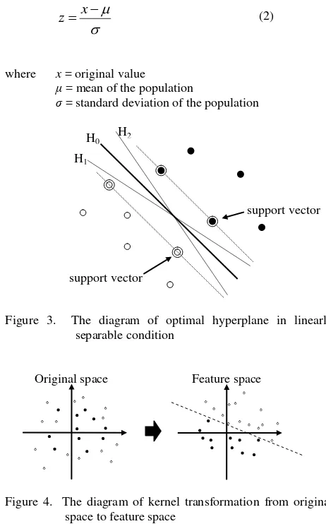
3.3.1 Support Vector Machine: SVM was a machine-learning method and developed by Vapnik (1998). In the linearly separable condition, it classifies the dataset by finding at least one hyperplane defined by support vector that can discriminate two classes (Figure 3: H0 - H2). The optimal hyperplane is that the distance between the closest training sample and the hyperplane was maximized (Figure 3: H0). If it cannot be discriminated linearly, it will input into high-dimensional feature space by kernel transformation to find the linearly separable condition (Melgani and Bruzzone, 2004), as shown in Figure 4. The kernel function available in the software included linear, polynomial, radial basis function (RBF), and sigmoid, they will be chosen based on the distribution of data. The kernel function we used was RBF that had been demonstrated suitable for most conditions. In this model, all input variable had been standardized to Z-score:
σ= standard deviation of the population
Figure 3. The diagram of optimal hyperplane in linearly
3.3.2 Maximum Entropy: MAXENT can make predictions from incomplete information (Phillips et al., 2006), and may remain effective from small sample sizes (Kumar and Stohlgren, 2009). The principle of MAXENT is based on the concepts of entropy in thermodynamic, referred to as the measure of disorder, and then is used to described the probability distribution in several domains, and Bayesian statistics is for exploring the probability distribution of each pixel when the
L = linear Predictor Normalizer
Z = a scaling constant that ensures that P sums to 1 over all grid cells
MAXENT software is freely available on the worldwide web (http://www.cs.princeton.edu/~schapire /MAXENT).
3.3.3 Decision Tree: DT (also called Classification and Regression Trees, CART) is a non-parametric classification algorithm for data mining with both classifying and predicting capability. DT could build classified rules from observations or some experiences (Guisan and Zimmermann, 2000). Decision tree algorithm sequentially partitions the dataset with some important predictors in order to maximize differences on a dependent variable. As show in Figure 5, the decision pathways originate from a starting node (root) that contains all observations, then classify step by step into binary subsets based on the important predictors, and so on. Finally, it will end at multiple nodes containing unique subsets of observations. Terminal nodes are assigned a final outcome based on group
membership of the majority of observations (De’ath and
Fabricius, 2000; Bourg et al., 2005; O’Brien et al., 2005). DT was implemented by using SPSS CRT software module.
Figure 5. The diagram of the classified process of DT Population
3.4 Model Validation
Accuracy assessment contains the overall accuracy and kappa coefficient of agreement of the predictions for two species. The kappa coefficient is a measure of agreement between predictive values and observations. The kappa value of 1.0 indicates a perfect agreement and the value of 0.0 indicates an agreement equivalent to chance (Viera and Garrett, 2005), and the value higher than 0.8 indicate a stronger agreement and the value lower than 0.4 indicate a poorer agreement (Jensen, 2005).
4. RESULTS AND DISCUSSION
As shown in the LB case of Table 6, the accuracies of SVM and DT with test set 1 were slightly higher than that of MAXENT. Nevertheless, the kappa values of all three models were higher than 0.8, it means that they had a stronger agreement. However, the ability of extrapolation (Test Set 2) was poor for all three models, with kappa values lower than 0.6, where MAXENT was the worst, with a value of 0.38. The main reason is that these models were built merely based on topographic factors that affect the growth of plant indirectly. The effect of directly operating factors, like microclimate, could not be derived from topographic factors, thereby making the models unable to simulate the species’ growth in different areas.
As shown in the HB case of Table 6, MAXENT kept high kappa values (0.85, Test Set 1), whereas those of SVM (0.61) and DT (0.57) models declined significantly. The lower kappa value in Training Set resulted from more commission errors with a larger background sample size. In terms of accuracy, MAXENT will take the accuracies of both target and background samples into account; whereas SVM and DT will tend to raise the accuracies of background samples, thereby reducing the accuracies of target samples and overall accuracies. In the respect of statistical characteristics, MAXENT calculates the probability distribution by entropy that attempts to find the maximum present probability in nature, which is close to the status of ecology, and considering the background samples with lower probability instead of viewing as absences for taking account of overall distribution of target samples, thus resulting in higher accuracy on extrapolation. Since SVM and DT are developed based on mathematical concepts, they will divide each class as complete as possible. Thus, more disperse or confused information in samples or more background samples incorporated in the models, more fragmentary or convergent area will been predicted either in SVM or DT models. The predictions of SVM and DT in HB cases resulted in not only underestimating potential habitat but also unreasonable conditions in reality. For example, in the prediction of DT in
range around the samples at hand, they were hard to extrapolate to the area that we do not have any samples.
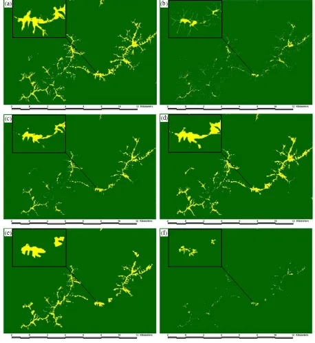
Figure 7 shows the area of potential habitat of three models with low and high biodiversity. In MAXENT model, the area of potential habitat increased slightly when it was in high biodiversity (large background size). It attributed to that MAXENT would attempt to keep the overall distribution of the target samples. The predictions of SVM and DT models resulted in that the area of potential habitat tended to very concentrated and fragmentary in the HB cases, especially in DT models. These two models would tend to underestimate the potential habitat, thereby limiting the ability of extrapolation. However, these results had the potential to find out the area with the highest probability of presence in where the environment was extremely close to that in the existed samples. It was still very useful for reducing the area of species field survey to save much time and labor.
Model LB HB
Table 6. The accuracies of models with low biodiversity (LB) and high (HB) biodiversity
5. CONCLUSIONS
The accuracies of all three models had excellent capability on predicting the potential habitat in low biodiversity (kappa > 0.8). However, only MAXENT could keep the excellent prediction in high biodiversity; whereas SVM and DT models would be too convergent, thereby underestimating the potential habitat.
Therefore, we conclude that MAXENT is the best one for predicting the species’ potential suitable habitat to assist the decision-making of plantation, reforestation, or recovery. In contrast, the prediction of SVM and DT models would underestimate species distribution significantly, and thus limit the ability of extrapolation, but they still could be used to find out the area with the highest probability of species’ presence to assist species field survey or restoration selection of rare species.
In future, to predict more accurately, we will consider about other factors that are more directly related to the growth of species, like shade or solar illumination factors, to improve the predictions of models. And we will also use the classification maps derived from LIDAR or hyperspectral imagery to identify different species precisely to promote the predictive capability of models in more detail.
Figure 7. The maps of potential habitat of LLCs predicted by three models: (a) SVM, LB;(b) SVM, HB;(c) MAXENT, LB;(d) MAXENT, HB;(e) DT, LB;(f) DT, HB. The insets over the up-left are a part of entire area for showing the details of the maps.
6. REFERENCES
Bourg, N. A., Mcshea, W. J., and Gill, D. E., 2005. Putting a CART before search: successful habitat prediction for a rare forest herb. Ecology, 86(10), pp. 2793-2804
Dalponte, M., Bruzzone, L., and Gianelle, D., 2008. Fusion of hyperspectral and LIDAR remote sensing data for classification of complex forest areas. IEEE Transactions on Geoscience and Remote Sensing, 46(5), pp. 1416-1427.
De’ath, G. and Fabricius, K. E., 2000. Classification and regression trees: a powerful yet simple technique for ecological data analysis. Ecology, 81 (11), pp. 3178-3192.
Drake, J. M., Randin, C., and Guisan, A, 2006. Modelling ecological niches with support vector machines. Journal of Applied Ecology, 43, pp. 424-432.
Elith, J., Graham, C. H., Anderson, R. P., Dudík, M., Ferrier, S., Guisan, A., Hijmans, R. J., Huettmann, F., Leathwick, J. R., Lehmann, A., Li, J., Lohmann, L, G., Loiselle, B, A., Manion, G., Moritz, C., Nakamura, M., Nakazawa, Y., Overton, J. McC., Peterson, A. T., Phillips, S. J., Richardson, K., Scachetti-Pereira, (b)
(a)
(e) (f)
(c) (d)
R., Schapire, R. E., Soberón, J., Williams, S., Wisz, M. S., and Zimmermann, N. E., 2006. Novel methods improve prediction
of species’ distributions from occurrence data. ECOGRAPHY, 29, pp. 129-151.
Felicísimo, A. M. and Gómez-Muñoz, A., 2004. GIS and predictive modeling: a comparison of methods applied to forestal management and decision-making. Proceedings of GIS Research UK, pp. 143-144.
Guisan, A. and Zimmermann, N. E., 2000. Predictive habitat distribution models in ecology. Ecological Modeling, 135, pp. 147-186.
Guo, Q., Kelly, M., and Graham, C. H., 2005. Support vector machines for predicting distribution of Sudden Oak Death in California. Ecological Modelling,182(2005), pp. 75-90.
Hernandez, P. A., Graham, C. H., Master, L. L., and Albert, D. L., 2006. The effect of sample size and species characteristics on performance of different species distribution modeling methods. ECOGRAPHY, 29, pp. 773-785.
Hoffer, R. M., 1978. Biological and physical considerations in applying computer-aided analysis techniques to remote sensor data. In: Swain, P. H. and S. M. Davis (Eds.), Remote Sensing: The Quantitative Approach, McGraw-Hill, Inc., New York, pp. 227-289.
Jensen, J. R., 2005. Introductory Digital Image Processing: A Remote Sensing Perspective, 3rd Edition. Pearson Education, Inc., New Jersey, pp. 506-508.
Kumar, S. and Stohlgren, T. J., 2009. Maxent modeling for predicting suitable habitat for threatened and endangered tree Canacomyrica monticola in New Caledonia. Journal of Ecology and Natural Environment, 1(4), pp. 94-98.
Landenburger, L., Lawrence, R. L., Podruzny, S., and Schwartz, C. C., 2008. Mapping regional distribution of a single tree species: white bark pine in the Greater Yellowstone Ecosystem. Sensors, 8, pp. 4983-4994.
Melgani, F. and Bruzzone, Lorenzo, 2004. Classification of Hyperspectral Remote Sensing Images With Support Vector Machines. IEEE Transactions on Geoscience and Remote Sensing, 42(8), pp. 1778-1790.
Miller, J. R., Turner, M. G., Smithwick, E. A. H., Dent, C. L., and Stanley, E. H., 2004. Spatial extrapolation: the science of predicting ecological patterns and processes. BioScience, 54 (4), pp. 310-320.
O’Brien, C. S., Rosenstock, S. S., Hervert, J. J., Bright, J. L.,
and Boe, S. R., 2005. Landscape – level models of potential habitat for Sonoran pronghorn. Wildlife Society Bulletin, 33 (1), pp. 24-34.
Peterson, A. T., Papeş, M., and Eaton, M., 2007. Transferability and model evaluation in ecological niche modeling: a comparison of GARP and Maxent. Ecography, 30, pp. 550-560.
Pereira, J. M. C. and Itami, R. M., 1991. GIS-based habitat modeling using logistic multiple regression: a study of the Mt. Graham red squirrel. Photogrammetric Engineering & Remote Sensing, 57 (11), pp. 1475-1486.
Phillips, S. J., Anderson, R. P., and Schapire, R. E., 2006. Maximum entropy modeling of species geographic distributions. Ecol. Model, 190, pp. 231-259.
Skidmore, A. K., 1990. Terrain position as mapped from a gridded digital elevation model. International Journal of Geographical Information Systems, 4(1), pp. 33-49.
Sperduto, M. B. and Congalton, R. G., 1996. Predicting rare orchid (small Whorled Pogonia) habitat using GIS. Photogrammetric Engineering & Remote Sensing, 62 (11), pp. 1269-1279.
Vapnik,V. N., 1998. Statistical Learning Theory. Hoboken, NJ: Wiley.
Viera, A. J. and Garrett, J. M., 2005. Understanding interobserver agreement: the kappa statistic. Family Medicine, 37(5), pp. 360-363.