A PLUGIN TO INTERFACE OPENMODELLER FROM QGIS FOR SPECIES’
POTENTIAL DISTRIBUTION MODELLING
Daniel Beckera,∗, Christian Willmesa, Georg Baretha, Gerd-Christian Wenigerb
a
Institute of Geography, University of Cologne, Albertus-Magnus-Platz, 50923 Cologne, Germany (daniel.becker, c.willmes, g.bareth)@uni-koeln.de
b
Neanderthal Museum, Talstraße 300, 40822 Mettmann, Germany [email protected]
Commission VII, SpS10 - FOSS4G: FOSS4G Session (coorganized with OSGeo)
KEY WORDS:openModeller, QGIS, Python, Plugin, Ecological Niche Modelling, ENM, Species Potential Distribution Modelling, SPDM
ABSTRACT:
This contribution describes the development of a plugin for the geographic information system QGIS to interface the openModeller software package. The aim is to use openModeller to generate species’ potential distribution models for various archaeological ap-plications (site catchment analysis, for example). Since the usage of openModeller’s command-line interface and configuration files can be a bit inconvenient, an extension of the QGIS user interface to handle these tasks, in combination with the management of the geographic data, was required. The implementation was realized in Python using PyQGIS and PyQT. The plugin, in combination with QGIS, handles the tasks of managing geographical data, data conversion, generation of configuration files required by openModeller and compilation of a project folder. The plugin proved to be very helpful with the task of compiling project datasets and configuration files for multiple instances of species occurrence datasets and the overall handling of openModeller. In addition, the plugin is easily extensible to take potential new requirements into account in the future.
1. INTRODUCTION
The work presented here is realized in the context of the inter-disciplinary research project Collaborative Research Centre 806 (CRC8061). The main topic of the CRC806 is entitled ”Our Way to Europe” and one of the main objectives of it, is to capture the complex nature of chronology, regional structure, climatic, envi-ronmental and socio-cultural contexts in Europe during the last 190.000 years by interdisciplinary research (Richter et al., 2012).
The overall context of this work is the modelling of ecological niches (ENM) or species’ potential distributions (SPDM) of var-ious faunal species for the Upper Palaeolithic (50-10 kyBP). The results are planned to be used as data to investigate if findings of faunal remains at archaeological sites on the Iberian Penin-sula are associated with the modelled distributions. The main study area of the project C1 is the Iberian Peninsula, its discussed role as a refuge for Neanderthals and the replacement process of Neanderthals by anatomically modern humans (Weniger and Re-icherter, 2015).
OpenModeller (de Souza Mu˜noz et al., 2011) is a cross-platform environment to carry out ecological niche modelling experiments, that was built with the motivation to provide a single expand-able open source platform for ENM or SPDM with different al-gorithms. The extensibility, cross-platform capabilities, the pos-sibility to apply and compare multiple modelling algorithms as well as the ability to project the modelling results to environ-mental data of a different time slice in particular, are the reasons openModeller was picked for this purpose. Based on the fact that the desktop GUI version was not updated since 2010 and that the original QGIS plugin is not available anymore for the current
∗Corresponding author
1http://www.sfb806.de
version of QGIS, and that the manual editing of the configuration files is relatively complicated, a GUI for more comfortable, effec-tive handling and generation of the input data was required. This work presents a QGIS plugin we developed for this purpose and exemplary results that were accomplished using openModeller in combination with the plugin.
In the following section 2. the terminology of the modelling ap-proach is explained, as well as related work concerning SPDM and the openModeller application while the focus of this contri-bution is on the presentation of the QGIS plugin. Section 3. ex-plains the software used to implement the plugin and the data and modelling algorithm applied to produce the example results. In section 4. the data import and cartography is documented briefly and the implementation of the plugin and its functionalities are explained. The user interface and work flow of the plugin is ex-plained in section 5., as well as a short presentation of an exem-plary SPD-model, that are both discussed in section 6..
2. CONCEPTS AND RELATED WORK
Within the C1 and Z2 project (2) of the CRC806, GIS-supported site catchment analysis (Vita-Finzi and Higgs, 1970, Becker, 2012) (SCA) is applied to palaeolithic sites in northern Spain to anal-yse the relationship between the sites inhabitants and their envi-ronment (Ullah, 2011) and the resources in the sites economic range (Legg, 2008). To enable further analysis of potential prey species in the sites environment and investigation of a possible relationship to the actual on-site findings of faunal remains, ex-tensive data about potential faunal distribution of various species is assumed to be useful. The basic idea is that hunter-gatherer economies and lifestyles were tied to the distributions of faunal
and floral resources (and resources of inanimate nature) while those were themselves influenced by changes in the environment (Franklin et al., 2015, Gravel-Miguel, 2015). Overall it is valu-able to reconstruct past environments to understand economic be-haviours and mobility of hunter-gatherers.
To generate faunal palaeodistribution data, species’ potential dis-tribution modelling (SPDM) (Phillips et al., 2006) is applied, uti-lizing the openModeller software package. It appears that the exact terminology is still in debate and that the terms ecologi-cal niche modelling (ENM) and species distribution modelling (SDM) are often used inappropriately without the required dis-tinction (Peterson and Sober´on, 2012, Elith and Leathwick, 2009). This contribution settles for the terminology used by the team be-hind openModeller (SPDM) in the related publication (de Souza Mu˜noz et al., 2011). The key assumption of these approaches is that a species’ distribution depends on their environment since specific environmental variables allow long-term survival of a species (Phillips et al., 2006). The modelling approach uses ob-servations of species at locations as the dependent variable, while the environmental factors are treated as explanatory variables (Elith and Franklin, 2013). Since the goal is the modelling of species potential palaeodistributions, appropriate environmental data is necessary and available in the form of climate data that should be used to project present species occurrences to past potential distributions. OpenModeller provides multiple model algorithms like Maxent, GARP & Bioclim. This contribution limits the re-sults to an example modelled with the Maxent modelling algo-rithm.
3. DATA AND METHODS
The data and methods used for the species’ potential distribution modelling, as well as the tools used for the plugin development are introduced in this section.
3.1 Occurrence and Environmental Data
To accomplish the modelling process with openModeller, species occurrence data (also: ”presence data”) is needed. The source for the used occurrence data is the Global Biodiversity Information Facility (GBIF Secretariat: GBIF Backbone Taxonomy, 2013), which is an extensive source for records of various organisms. The data is provided as CSV text files, as Darwin Core Archives (TDWG Task Group, 2009) or via an API to retrieve the datasets directly. The files contain latitude/longitude coordinates for the points of occurrence and further data on the species and were converted to shapefiles with QGIS to enable simpler handling of the data.
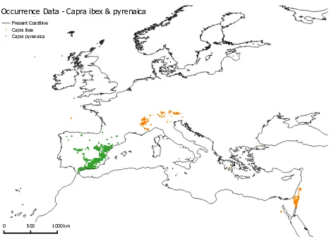
Concerning the selection of species for the modelling approach, there are multiple candidates that qualify for SPDM in this ar-chaeological context (including recent distribution), such as wild boar, red deer, roe deer or bison (Gravel-Miguel, 2015). For now it was decided to apply the work flow on Capra (also: ”Ibex”). Because of the localization on or in the proximity of the Iberian Peninsula, the modelling process was run for Capra ibex and Capra pyrenaica for the exemplary results.
The modelling process relies on a second set of variables, the en-vironmental data. A subset of the ’bioclimatic’ variables of the WorldClim global climate data collection was used for this pur-pose (Hijmans et al., 2005). The climate data for the Last Glacial Maximum (21 kyBP) is available in 2.5 arc-minute resolution. The bioclimatic variables are derived from monthly temperature and rainfall values with the aim to generate variables that are more biologically meaningful than the raw climate data. Since
Present Coastline Capra ibex Capra pyrenaica
0 500 1000 km
Occurrence Data - Capra ibex & pyrenaica
Figure 1: Occurrence Data for Capra ibex and Capra pyrenaica. (GBIF Secretariat: GBIF Backbone Taxonomy, 2013)
the modelling for this work was mainly done for first testing pur-poses, the complete set of bioclimatic variables (BIO 1-19) of the MPI-ESM-P model data was selected to conduct the modelling. Further, the 2014 version of GEBCO (General Bathymetric Chart of the Oceans 2014, 2014) was used as the source for the topo-graphic data, in the form of elevation and aspect rasters, to be able to take account of the changed sea-level in the LGM.
3.2 openModeller & QGIS
The openModeller software package is used for the actual SPDM modelling process. OpenModeller is very well suited for the use case presented here, since it allows to easily project recent species distributions to different scenarios, based on different palaeoenvi-ronmental data of various time slices such as the LGM mentioned above. The purpose for developing the openModeller framework was to perform the most common tasks related to species’ po-tential distribution modelling that are based on a correlative ap-proach. The open and modular architecture of openModeller al-lows it to implement new modelling algorithms as plugins that use the core modelling components via a defined interface (de Souza Mu˜noz et al., 2011). OpenModeller uses species occur-rence and environmental data to produce the species’ potential distribution models. The fact that these datasets are of geospatial nature suggests to use a geographic information system (GIS) for the data management and, in consequence, the configuration of the command line based openModeller software. Various inter-faces, SWIG python bindings for example, allow different client applications to interact with openModeller. For now, this di-rect implementation was not pursued, instead the included shell-programs are utilized and the associated configuration files are generated with the presented plugin. QGIS came to mind first, be-cause a now deprecated plugin already exists for an older version (<2.0) of QGIS and was ultimately selected because it satisfies all the demands necessary for the task at hand and its expandabil-ity through the very well documented PyQGIS and PyQT APIs that provide an excellent option to build UI-based plugins for QGIS.
3.3 The modelling algorithm
of ENM or SPDM these constraints consist of the range of en-vironmental data where the species occur, while the occurrence points of the species serve as the sample points (Phillips et al., 2006, Townsend Peterson et al., 2007). Maxent is also the name of a software package, which was presented in 2006 (Phillips et al., 2006) to perform maximum entropy modelling with georef-erenced occurrence data and environmental variables and the al-gorithm was later implemented in openModeller. The Maxent implementation in openModeller produces a continuous raster in various output file types that represent cumulative probabilities of occurrence (Phillips et al., 2006). In this application, integer type rasters with value ranges from 0-100 are used.
4. IMPLEMENTATION
The data import is explained briefly in this section, followed by a detailed description of the functionalities and the implementation of the presented plugin and a short summary of the cartography.
4.1 Data Import
The occurrence data was retrieved from GBIF (GBIF Secretariat: GBIF Backbone Taxonomy, 2013) as .csv files. Besides data about the species classification, binomial name, recording entity etc., the file contains geographic coordinates in decimal latitude/-longitude. The tool ”Create a Layer from a Delimited Text File” was used to convert the .csv file(s) to a point-type shapefile, which allows more simple handling with a GIS.
The bioclimatic datasets (Present & LGM) were downloaded in the .bil (Band Interleaved by Line) file format and converted to GeoTIFF files with QGIS as well, to ensure compatibility with openModeller, although openModeller should accept all file for-mats supported by GDAL (GDAL Development Team, 2015).
The netCDF version of the global GEBCO 2014 was downloaded and converted to GeoTIFF with gdal translate. To use coherent topographic data, the GEBCO 2014 data was used to produce landmass rasters mirroring the present day and the LGM sea-level (120m below today’s sea-sea-level (Clark and Mix, 2002). This was done with GRASS GIS r.mapcalc. The aspect rasters derived from the GEBCO DEM were computed using GDAL.
4.2 Plugin
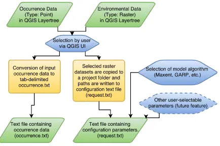
The plugin was implemented using PyQGIS and PyQT with the aid of ”Plugin Builder 2.8.1” (Sherman, 2015) as a starting point. QGIS Plugin Builder provides a working template from which a plugin can be built. The user interface was arranged with QT Designer. For now, the plugin is required to fulfill the follow-ing tasks (seen in figure 2 & 3 in section 5.): The openModeller om console.exe, which is used to conduct the modelling process, requires a text file ”occurrence.txt” with occurrence data and a configuration file ”request.txt”. The occurrence data is contained in the occurrence.txt, while the request.txt contains paths to the used environmental variables and further configuration parame-ters like the applied modelling algorithm, for example. The aim of the plugin is to generate these files with the aid of the QGIS user interface shown in figure 3 and conduct necessary file con-versions via the steps illustrated in the chart in figure 2 and ex-plained in the following segment:
• Select vector & raster layers in the QGIS layer tree to assign them to the appropriate categories.
– Point vector layer→occurrence data.
Figure 2: Chart of the plugins functionality.
– Raster data→environmental datasets.
• Allow selection of different modelling algorithms through the UI.
• Generate the occurrence.txt.
– The necessary columns (species label, longitude/lati-tude coordinates) are copied to the generated occur-rence.txt.
– In some cases it may be requested to generate a model for a whole genus instead of a species. The GBIF oc-currence files contain columns for ”genus” and ”species” and the plugin should allow switching between those.
– Multiple instances of occurrence layers can be added, one request.txt and one occurrence.txt is generated for every layer.
• Copy the environmental datasets into the project folder.
• Generate the request.txt.
– Paths to raster and vector files are copied to the ap-propriate place in the request.txt which generated with the necessary, selected parameters.
– The name of the occurrence layer is used for ”Occur-rences group” parameter, so it must match the ”species” or ”genus” string from the source data.
• If all files are copied and the text files are generated, the om console.exe can be executed with the respective request.txt as parameter and the model is computed.
4.3 Cartography
The cartography of the SPDM maps was realized with the QGIS (version 2.12) print composer. OpenModeller produces GeoTIFF raster files in which the probability of occurrence is stored with an integer value from 0 to 100 (other output formats are possi-ble, for example floating point 0-1) that were colored in evenly distributed classes. The coast lines for the present time slice are taken from the natural earth dataset (Kelso and Patterson, 2010), the lines for the LGM are constructed from the the GEBCO global bathymetry DEM (sea level -120m).
5. RESULTS
In this section the functionality of the plugin is explained briefly, followed by an example modelling result that was produced with the plugin and the before presented work flow and software.
5.1 Plugin
The general process allows the user to select one or multiple lay-ers in the QGIS layer tree, followed by a click on the respective button to load the layers into the list. The plugin allows the se-lection of multiple occurrence vector layers (figure 3a) with the result that one request.txt and a occurrence.txt is generated for every layer loaded into the list widget. Radio buttons (Figure 3a) allow switching between ”genus” and ”species”, for the data ex-port. The second list (figure 3b) should be filled with raster layers representing environmental data that builds the model, the before mentioned bioclimatic variables for the present time slice, for ex-ample. The mask layer list (figure 3c) sets three data points in the request.txt that delimit the modelling and projection area and define the format (e.g. resolution) of the output file containing the model data. The last list (figure 3d) should contain the en-vironmental variable layers that correspond to the datasets in the list in figure 3b. This can be the same set of data, or correspond-ing data for another time slice like the LGM, which results in the projection of the model to this explicit data. The output folder is selected as seen at 3e, while the model algorithm is selected with a combobox (figure 3f). The ”Generate” button starts the process of generating the folder structure, the configuration files and copying the data. The plugin is published in the CRC806 database (Willmes et al., 2014) where it can be acquired from (Becker and Willmes, 2015).
a
b
c
d
e f
Figure 3: Workflow of the Plugin. (a) This defines multiple oc-currence data layers, for every instance a request.txt and a occur-rence.txt is generated. (b) Defines the data that will be used to build the model. (c) Defines the raster datasets that are used as ”Mask” or ”Output format” & ”Output mask”. (d) These layers will be used to project the model. (e) Defines the destination path. Combobox (f) lets the user choose the modelling algorithm.
5.2 Examplary modelling results
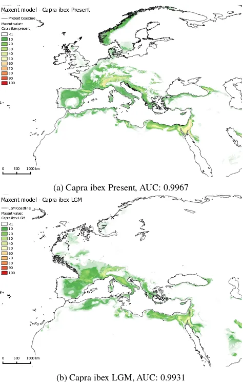
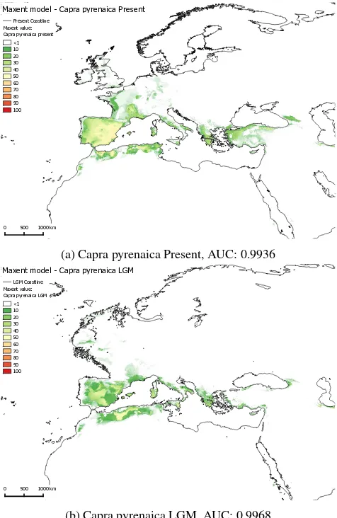
Figures 4a,4b,5a and 5b show maps visualizing the potential dis-tribution of Capra ibex and Capra pyrenaica modelled with open-Modeller’s Maxent implementation for two time slices (Present and LGM). The before explained bioclimatic and topographic datasets were used as environmental data (explanatory variable) for present and LGM climate conditions to project the model. The Maxent results are displayed in 10% classes, while discard-ing values<1 (white). The maps show an obvious impact of the data used for the different time slices, since even the lowest Max-ent values show a smaller overall area of potMax-ential distribution and strongly reduced probabilities of occurrence in the northern areas of the map, which were also glaciated in the LGM. Accord-ing to the area under the curve (AUC) values generated by open-Modeller, the models performed very well (Capra ibex present / LGM: 0.9936 / 0.9931; Capra pyrenaica present / LGM: 0.9967 / 0.9968).
The resulting models should fulfill their purpose to gain quantita-tive data about the palaeolithic fauna in the last glacial maximum, however, not without further classification and interpretation of the data, and with regard to the fact that the results are partly based on climate data from simulated model experiments as well. Nonetheless, the results should provide a valuable insight about this part of the LGM palaeoenvironment.
Present Coastline
Maxent value: Capra ibex present
<1 10 20 30 40 50 60 70 80 90 100
0 500 1000 km
Maxent model - Capra ibex Present
(a) Capra ibex Present, AUC: 0.9967
LGM Coastline Maxent value: Capra ibex LGM
<1 10 20 30 40 50 60 70 80 90 100
0 500 1000 km
Maxent model - Capra ibex LGM
(b) Capra ibex LGM, AUC: 0.9931
Present Coastline
Maxent model - Capra pyrenaica Present
(a) Capra pyrenaica Present, AUC: 0.9936
LGM Coastline
Maxent model - Capra pyrenaica LGM
(b) Capra pyrenaica LGM, AUC: 0.9968
Figure 5: Maps showing modelling results for Capra pyrenaica with Maxent values 1-100.
6. DISCUSSION AND CONCLUSIONS
The plugin presented in this work proved to be very helpful with the task of using multiple geographic datasets of occurrence and environmental data to produce a collection of input data and con-figuration files needed to control openModeller’s om console com-mand line program. QGIS is a perfectly suitable software envi-ronment to process the geographic input data, the combination with PyQGIS and the standard python abilities enables and sim-plifies potentially necessary file conversions or pre-processing. Thus, it was the right choice to implement the plugin for QGIS.
However, despite openModeller’s numerous benefits, like exten-sibility, versatility by supporting a wide variety of modelling al-gorithms, the ability to project results to other time slices with different input data, it seems that other options are utilized more often. While there are modelling studies (Jim´enez-Valverde et al., 2011, Dupin et al., 2011) that use multiple modeling algorithms, driven by various software packages (including openModeller) to compare and evaluate the results, surveys (Joppa et al., 2013, Ahmed et al., 2015) show that R and Maxent were the most com-monly used software packages within their sample, while open-Modeller was used in a few cases. Ahmed et al. (Ahmed et al., 2015) state that both software packages lie at opposing ends of the use-complexity spectrum, with Maxent as a point-and-click solu-tion and R being syntax-driven. We would estimate that open-Modeller is situated near the first category, with the advantage that it unifies the work flow and data management for multiple
modelling algorithms. The openModeller desktop version which is no longer maintained was especially comfortable to use, while the presented plugin is supposed to fill this gap.
The exemplary model results produced with openModeller ap-pear very promising as well, although further processing and in-terpretation of the data is necessary. Many species distribution modelling techniques produce continuous suitability values, but an application that wants to make quantitative assertions, like site catchment analysis, requires classified or binary (presence/ab-sence) output data (Liu et al., 2013). The necessary threshold selection or class definition is a separate problem that will be in-vestigated at another point.
ACKNOWLEDGEMENTS
This work was conducted within the Collaborative Research Cen-tre 806 (www.sfb806.de) which is funded by the German Re-search Foundation.
REFERENCES
Ahmed, S. E., McInerny, G., O’Hara, K., Harper, R., Salido, L., Emmott, S. and Joppa, L. N., 2015. Scientists and software - sur-veying the species distribution modelling community. Diversity and Distributions21(3), pp. 258–267.
Becker, D., 2012. GIS-basierte Distanzanalysen f¨ur die Model-lierung von Einzugsgebieten pr¨ahistorischer Fundst¨atten. Diplo-marbeit, University of Cologne. DOI: http://dx.doi.org/ 10.5880/SFB806.7, accessed: 2015-11-12.
Becker, D. and Willmes, C., 2015. A QGIS plugin to interface openModeller. CRC806-Database, DOI:http://dx.doi.org/ 10.5880/SFB806.16.
Clark, P. and Mix, A., 2002. Ice sheets and sea level of the Last Glacial Maximum.Quaternary Science Reviews21, pp. 1–7.
de Souza Mu˜noz, M. E., De Giovanni, R., de Siqueira, M. F., Sut-ton, T., Brewer, P., Pereira, R. S., Canhos, D. A. L. and Canhos, V. P., 2011. openModeller: a generic approach to species’ poten-tial distribution modelling.GeoInformatica15(1), pp. 111–135.
Dupin, M., Reynaud, P., Jaroˇs´ık, V., Baker, R., Brunel, S., Eyre, D., Pergl, J. and Makowski, D., 2011. Effects of the Training Dataset Characteristics on the Performance of Nine Species Dis-tribution Models: Application to Diabrotica virgifera virgifera.
PloS ONE6(6), pp. 1–11.
Elith, J. and Franklin, J., 2013. Species Distribution Modeling. In:Encyclopedia of Biodiversity, Elsevier, pp. 692–705.
Elith, J. and Leathwick, J. R., 2009. Species Distribution Mod-els: Ecological Explanation and Prediction Across Space and Time. Annual Review of Ecology, Evolution, and Systematics
40(1), pp. 677–697.
Franklin, J., Potts, A. J., Fisher, E. C., Cowling, R. M. and Marean, C. W., 2015. Paleodistribution modeling in archaeol-ogy and paleoanthropolarchaeol-ogy. Quaternary Science Reviews110, pp. 1–14.
GBIF Secretariat: GBIF Backbone Taxonomy, 2013. http:// www.gbif.org/species/2441047, accessed: 2015-10-30.
General Bathymetric Chart of the Oceans 2014, 2014.
http://www.gebco.net/data_and_products/gridded_ bathymetry_data/gebco_30_second_grid, accessed: 2015-11-17.
Gravel-Miguel, C., 2015. Using Species Distribution Model-ing to contextualize Lower Magdalenian social networks visible through portable art stylistic similarities in the Cantabrian region (Spain).Quaternary International. Article in press.
Hijmans, R. J., Cameron, S. E., Parra, J. L., Jones, P. G. and Jarvis, A., 2005. Very high resolution interpolated climate sur-faces for global land areas.International Journal of Climatology
25(15), pp. 1965–1978.
Jim´enez-Valverde, A., Decae, A. E. and Arnedo, M. a., 2011. Environmental suitability of new reported localities of the funnel-web spider Macrothele calpeiana: An assessment using potential distribution modelling with presence-only techniques.Journal of Biogeography38(6), pp. 1213–1223.
Joppa, L. N., McInerny, G., Harper, R., Salido, L., Takeda, K., O’Hara, K., Gavaghan, D. and Emmott, S., 2013. Troubling Trends in Scientific Software Use. Science340(6134), pp. 814– 815.
Kelso, N. V. and Patterson, T., 2010. Introducing Natural Earth Data - Naturalearthdata.com.Geographia Technicapp. 82–89.
Legg, R. J., 2008. Catchment Analysis. In: R. J. Legg (ed.),
Encyclopedia of Archaeology, Elsevier, pp. 2002–2004.
Liu, C., White, M. and Newell, G., 2013. Selecting thresholds for the prediction of species occurrence with presence-only data.
Journal of Biogeography40(4), pp. 778–789.
Peterson, A. T. and Sober´on, J., 2012. Species distribution mod-eling and ecological niche modmod-eling: Getting the Concepts Right.
Natureza a Conservacao10(2), pp. 102–107.
Phillips, S. J., Anderson, R. P. and Schapire, R. E., 2006. Maxi-mum entropy modeling of species geographic distributions. Eco-logical Modelling190(3-4), pp. 231–259.
Richter, J., Melles, M. and Sch¨abitz, F., 2012. Temporal and spatial corridors of Homo sapiens sapiens population dynamics during the Late Pleistocene and early Holocene. Quaternary In-ternational274, pp. 1–4.
Sherman, G., 2015. QGIS Plugin Builder.http://g-sherman. github.io/Qgis-Plugin-Builder/, accessed: 2015-11-03.
TDWG Task Group, 2009. The Darwin Core. http://www. tdwg.org/activities/darwincore/, accessed: 2015-11-25.
Townsend Peterson, A., Pape, M. and Eaton, M., 2007. Trans-ferability and model evaluation in ecological niche modeling: a comparison of GARP and Maxent. Ecography30(4), pp. 550– 560.
Ullah, I. I. T., 2011. A GIS method for assessing the zone of human-environmental impact around archaeological sites: a test case from the Late Neolithic of Wadi Ziqlˆab, Jordan. Journal of Archaeological Science38(3), pp. 623–632.
Vita-Finzi, C. and Higgs, E. S., 1970. Prehistoric economy in the Mount Carmel area of Palestine: site catchment analysis. 36, pp. 1–37.
Weniger, G.-C. and Reicherter, K., 2015. Collaborative Research Centre 806 - Project C1. http://www.sfb806.uni-koeln. de/index.php/projects/cluster-c/c1, accessed: 2015-10-25.
Willmes, C., K¨urner, D. and Bareth, G., 2014. Building Research Data Management Infrastructure using Open Source Software.