INTEGRATING GIS WITH AHP AND FUZZY LOGIC AHP TO GENERATE HAND,
FOOT AND MOUTH DISEASE HAZARD ZONATION (HFMD-HZ) MODEL IN
THAILAND
Ratchaphon Samphutthanon 1,*, Nitin Kumar Tripathi 1, Sarawut Ninsawat 1, Raphael Duboz 2
1 Remote Sensing and Geographic Information Systems Field of Study, School of Engineering and Technology, Asian Institute of Technology (AIT), Thailand; E-Mails: [email protected] (N.K.T); [email protected] (S.N.)
2 Agirs Research Unit, CIRAD, Montpellier, France; E-Mail: [email protected] (R.D.)
* Author to whom correspondence should be addressed;
E-Mail; [email protected]; Tel.:+66-2524-5799; Fax: +66-2524-5597.
KEY WORDS: Hand, Foot and Mouth Disease Hazard Zonation model (HFMD-HZ model); Spatial Multi-criteria Decision Analysis (SMCDA); Analytical Hierarchy Process (AHP); Fuzzy logic AHP; Geographic Information Systems (GIS).
ABSTRACT:
The main objective of this research was the development of an HFMD hazard zonation (HFMD-HZ) model by applying AHP and Fuzzy Logic AHP methodologies for weighting each spatial factor such as disease incidence, socio-economic and physical factors. The outputs of AHP and FAHP were input into a Geographic Information Systems (GIS) process for spatial analysis. 14 criteria were selected for analysis as important factors: disease incidence over 10 years from 2003 to 2012, population density, road density, land use and physical features. The results showed a consistency ratio (CR) value for these main criteria of 0.075427 for AHP, the CR for FAHP results was 0.092436. As both remained below the threshold of 0.1, the CR value were acceptable. After linking to actual geospatial data (disease incidence 2013) through spatial analysis by GIS for validation, the results of the FAHP approach were found to match more accurately than those of the AHP approach. The zones with the highest hazard of HFMD outbreaks were located in two main areas in central Muang Chiang Mai district including suburbs and Muang Chiang Rai district including the vicinity. The produced hazardous maps may be useful for organizing HFMD protection plans.
1. INTRODUCTION
HFMD has been known mostly in the northern region of Thailand for a long time. According to the figures of the Bureau of Epidemiology of the past 10 years, HFMD outbreaks occurred mainly in this region (Samphutthanon, 2014). Until now, effective chemoprophylaxis or vaccination approaches for dealing with HFMD are not available. HFMD is transmitted from one to others via direct contact with saliva, fluid from nose or blisters. In addition, it can also be caused by contact with food or water contaminated with fecal droplets, nose discharge, fluid or saliva of the infectious person.
Attempts to understand the disease are focused only on the study of medicine and public health or demographic distribution. However, understanding it in spatial terms is a different aspect that has not been established yet. Here, the application of GIS technology is useful in spatial analysis concerning medical and public health. The integration of GIS with an AHP using MCDM techniques has been applied to many fields. An AHP is applied to assign the weights of each criterion (Saaty, 1980). Determination of weights in AHP depends on a pairwise rank matrix. Systematic decision making analysis supports decision makers in effective summarizing of all relevant information. An AHP method was chosen for receiving parameter weights because of its simple hierarchical structure, mathematical basis, widespread usage and its ability to measure inconsistencies in judgments. AHP is a popular technique in decision making processes. It can also measure an abstract weight and convert it to concrete or numbers. The
resulting factor weights of the AHP calculation are entered into a main and sub factor analyses by spatial analysis in GIS. An alternative to AHP named Fuzzy Logic AHP was operated for conquer the offset method and the incompetence of the AHP in managing with linguistic variables. The FAHP approach enables a higher flexibility in the decision making process.
The results of the spatial analysis in GIS with AHP and FAHP may prove useful for planning protection measures before an actual outbreak. The reliability of the technical analysis was tested by validation with actual data of disease incidence in 2013. Thus, the accuracy of the results of the generated model could be confirmed.
2. STUDY AREA
The study area of this research is Northern region of Thailand. The geographic coordinate location is Longitude between 97° 19’ 8”E - 101° 22’ 18” E and Latitude between 17° 11’ 12”N - 20° 29’ 1”N. An area covering 93,690.85 sq.km. (9,300 hectares) or 18.25 percent of area in whole Thailand. There are 6,133,208 total population. This area consist of 9 provinces; Mae Hong Son, Chiang Mai, Chiang Rai, Lampun, Lampang, Phayao, Phrae, Nan and Uttraradit province. The relative location within north side connected to Republic of the Union of Myanmar and Laos PDR. East side connected to Laos PDR. West side connected to Republic of the Union of Myanmar and south side connected to Tak, Sukhothai and Pitsanulok province.
Figure 1 Study area: Northern of Thailand
3. METHODOLOGY
The main objective of the study is developing the HFMD hazard zonation model based on the Analytical Hierarchy Process (AHP) and Fuzzy Logic AHP with Geographic Information Systems (GIS). Then comparing the result of AHP and Fuzzy AHP approach with validate data. It can be separated in three main part analysis that consist of AHP calculation, Fuzzy logic AHP calculation and GIS analysis
3.1 Analytic Hierarchy Process (AHP) approach
Presently, AHP is the most popular decision process in multi criteria decision analysis. It builds on the rule of an additive decision that permits the problem structuring in a hierarchy and supply a good device for the decision analysis procession. The AHP components structure has the final target on the top, next below is a number of objectives then attributes and the last is alternatives (Figure 2). In the AHP applied here, the other choices are shown in the databases of GIS while each layer comprisesthe attribute values consigned to the alternatives then each alternative is associated to the attributes in higher level. (Malczewski, 1999).
Figure 2 The hierarchical structure of AHP decision making process (Kordi M. and Brandt S.A., 2012)
The AHP method was created by Saaty (L.T. Saaty,1980). Generally, AHP is specify the relative importance of criteria in multi-criteria decision making problems. AHP is a powerful and flexible decision making process to help people set priorities and make the best decision. The purpose of AHP is to express the importance of each factor relative to the other factors. This process has ability to judge qualitative criteria with quantitative criteria (Boroushaki and Malczewski, 2008). The AHP method has six steps for evaluating alternatives show in Figure 3. (C.H. Cheng et. al., 1999)
Figure 3 AHP process of evaluation alternatives
Step 1: Define the unstructured problem, identification of input or output parameters. The unstructured problem and their characters should be recognized the objectives and outcomes stated clearly.
Step 2: Generate a hierarchy structure, After AHP procedure in decompose decision problem in a hierarchy. This step the complex problem is decomposed in a hierarchical structure with decision elements which are objective, attributes such as criterion map layers and alternatives.
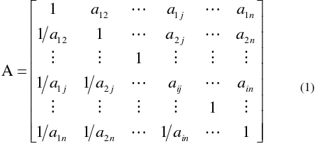
Step 3: Create pairwise comparison matrices, Each element of the hierarchy structure related elements in low hierarchy are linked in pairwise comparison matrices as follows:
1
1
1
1
1
1
1
1
1
1
1
A
2 1
2 1
2 2
12
1 1
12
in n
n
in ij
j j
n j
n j
a
a
a
a
a
a
a
a
a
a
a
a
a
(1)
Then, use geometric mean technique to define the geometric mean of each
a
ij for the final matrix Let k be the amount ofexpert and
a
ijb be the pairwise comparison value of dimensioni
factor toj
given by expert b, where b = 1, 2,…, kand
i,
j
1,2,....,
n
. After that, calculated the final matrixA as following in equation (2), where
x
ijis a geometric mean of AHP comparison value of dimensioni
factor toj
for allexpert, where
i,
j
1,2,....,
n
.
k
kij b
ij ij
ij
ij
a
a
a
a
x
1
2
...
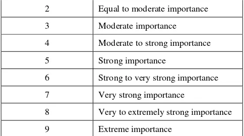
1 2)In order to define the relative preferences for two elements of the hierarchy in matrix A, an underlying meaning scale is applies with values from 1 to 9 to rate (Table 1).
Table 1 Scales for pairwise comparison (Saaty, 1980) Preferences expressed
in numeric variables
Preferences expressed in linguistic variables
1 Equal importance
2 Equal to moderate importance
3 Moderate importance
4 Moderate to strong importance
5 Strong importance
6 Strong to very strong importance
7 Very strong importance
8 Very to extremely strong importance
9 Extreme importance
Step 4: Estimate the relative weights
The eigenvalue method used to calculate the relative weight of element in each pairwise matrix. The relative weight of matrix is achieved from following equation:
Compute the factor weights. Let n and m be the number of
calculated the factor weight (
w
i) using equation (3).
Estimate the consistency ratio (CR) to ensure that the judgments of experts are consistent. Let n be the number of factor and
max
be the average value of the consistency vector (CV).Then, calculated the CV and
maxas following in equation (4) and (5), respectively:
Step 5: Test the consistency ratios
The consistency property of matrices is test to ensure that the decision maker judgments are consistent. The pre parameter is necessary. Consistency Index calculate by following equation:
1
The consistency index of a randomly generated reciprocal matrix be called the random index or RI, with reciprocals forced. An average RI for the matrices of order 1–15 was generated by using a sample size of 100 (Nobre et. al., 1999). The table of random indexes of the matrices of order 1–15 can be seen in Table 2 (Saaty, 1980). The last ratio that has to be calculated is Consistency Ratio or CR. Generally, if CR is less than 0.1, the judgments are consistent, so the derived weights can be used by the following formula:
RI
Step 6: Priority of an alternative by weights composition The last step, the relative weights of decision elements are collected to obtain in overall rating as follows equation:
m = number of attribute, n = number of site3.2 Fuzzy Logic Analytic Hierarchy Process (Fuzzy AHP) approach
Fuzzy logic is used to improve accuracy and reduce uncertainty of human thinking. One of the methods for modeling uncertainty is fuzzy logic (Zadeh, 1965). The Fuzzy AHP uses linguistic expression. It uses fuzzy logic for determining pairwise comparison matrix even AHP can not needed for modeling uncertainty in the decision maker opinions (Mikhailov, 2003). Extent analysis method is used in this research since the steps of this approach are easier than the other Fuzzy AHP approaches (Gumus, 2009 and Chang, 1996). The principle of Fuzzy AHP extent analysis method is a fuzzy number M on R to be a triangular fuzzy number (TFN) if their membership function
M
x
:
R
0
,
1
is equal to following equation (9):
0 fuzzy number by convention.
Figure 4 Membership functions of the triangular fuzzy number.
Table 3 Memberships function of linguistic scale for Triangle Fuzzynumber (Gumus, 2009).
Fuzzy Number Triangular Membership Number
1 (1,1,1) main steps; construct the pairwise comparison matrix and calculate priority weights.
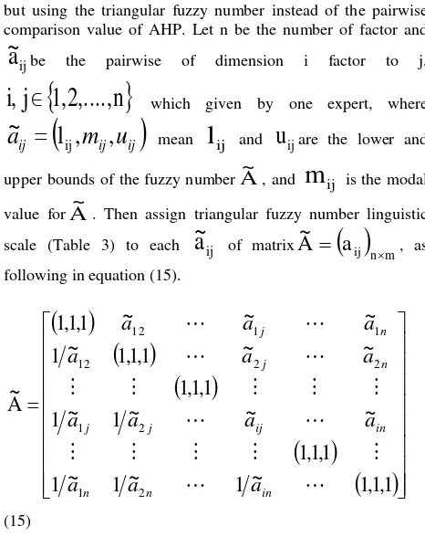
Construct the pairwise comparison matrix among the entire factor. Fuzzy AHP is constructed the pairwise comparison matrix based on the same data set of classical AHP approach,
following in equation (15).
pairwise comparison value of dimensioni
factor toj
given by expert b, where b = 1, 2,…, k andi,
j
1,2,....,
n
. After that, calculated the final pairwise comparison matrix as following in equation (16), where~
x
ijis a geometric mean ofCalculate priority weights. Let 1g
i fuzzy synthetic extent with respect to the ith object is defined as following in equation (17):
of each factor. This expression can be rewritten as following in equation (19):Figure 5 Intersection between
M
1andM
2To compare
M
1andM
2, the values ofV
M
1
M
2
and
V
M
2
M
1
are need. The degree possibility for a convex fuzzy number to be greater than k convex fuzzy numbers
i
1
,
2
,...,
k
Then the weight vector is given by
Through normalization, the weight vectors are normalized by equation (23):
3.3 Multi-criteria Decision Analysis (MCDA) with GIS Traditional MCDA techniques were used to analyze non-spatial data. In a real world situation, it cannot be assumed that the whole study area is spatially homogenous, because the evaluation criteria vary across space (R. Banai, 1993). The combination of MCDA techniques with GIS has advanced to the optimum evaluation alternative (J.R. Eastman, 1997).
MCDA combined with GIS is a decision making process examining geospatial data to provide more information for decision makers (J. Malczewski, 2006). To combine MCDA with GIS, each of the criteria would be displayed by a map (J. Malczewski, 1999). In GIS technology, generally the alternatives are selections of points, lines and polygons attached to such a map of criteria (M.H. Vahidnia et. al., 2008). GIS can be used to compare spatial phenomena and analyze their spatial relationship and thus enables policy makers to connect different information sources, perform complex analyses, imagin trends, project results and plan long term target (J. Malczewski, 2004).
MCDA combined with GIS is a process which merges and converts the inputs of a criteria map to a decision as the output. This process comprises of processes which link to geo spatial data, the decision maker's prefer and the data manipulation to a specified transformation into final ranking values of alternatives (A. Farkas, 2009).
In this case, the results of MCDA by AHP and Fuzzy logic AHP were linked to geospatial data from GIS. The outputs of MCDA were subjected to GIS analysis to weight each main and sub-criteria and generate a hazard zonation model by an overlay process. The overlay techniques were developed because in case of mapping and combining large datasets, the manual approach is limited. (Steinitz et. al., 1976). The WLC was introduced to create a risk map consisting of various zones.
4. MATERIAL OF CRITERIA LAYERS FOR ANALYSIS The criteria important for hazard zonation analysis consist of 3 main groups; 1) disease incidence 2) socio-economic and 3) physical features. The disease incidence datacover the 10 years from 2003 to 2012. The socio-economic data comprise population density, road density and landuse. The physical features concern topography. Each main criteria has a different weighthing volume and sub criteria were also weighted differently. The output of weight calculation by AHP and Fuzzy AHP was input to the geospatial database of spatial features
Figure 6 Criteria for analysis 4.1 Spatial disease incidence
The disease incidence was derived by calculating the ratio between the number of HFMD patients and the population of each village from 2003 to 2012, which was then subjected to an empirical bays smoothing process and Kernel Density Estimate (KDE). The results were classified in 5 levels. The maximum value is associated with the highest incidence and vice versa. The disease incidence in 2013 was derived by the same approach but it was validated by the results of the HFMD-HZ model from both AHP and Fuzzy AHP approach. The HFMD data were obtained from the Bureau of Epidemiology, Ministry of Public Health of Thailand, the population data from the Department of Provincial Administration, Ministry of Interior of Thailand. The village points were obtained from GISTDA, Ministry of Science and Technology of Thailand.
4.2 Socio-economic 4.2.1 Population density
Population density was calculated as population number divided by the area (person/sq.km.) for each sub district. The highest densities occurred in the capital (Mueang) districts of the provinces with the biggest clusters in Chiang Mai and Lampang. The lowest population density was found in Mae Hong Son province. High population density was attributed a high weight value as it implies a higher probability of close contact between persons and thus the spread of HFMD. This assumtion underlied the priority risk rating in 5 categories by population density with the highest population density indicating the highest risk of an outbreak and vice versa. The population data were gained from Department of Provincial Administration. The sub district data were obtained from GISTDA, Ministry of Science and Technology of Thailand.
4.2.2 Road density
Although this factor does not directly tell about contact intensity between people, it was interesting to analyze as a potential factor. An area with high road density might imply more crowded places such as markets, shops, restaurants, schools, nurseries or others that promote gathering. Therefore, for generating the HFMD-HZ model, the road density was classified into 5 classes with high road density rated highest. The road network database was obtained from the Department of Highways, Ministry of Transportation of Thailand.
4.2.3 Landuse
Landuse as of 2010 was interpreted from Landsat5 satellite data gathered by the Department of Land Development. Landuse was classified into many types. These were grouped into 5 categories as agricultural, built-up, forest, mixed forest areas and water bodies. The risk rating was determined by landuse features implying the intensity of human activities, with the highest rate attributed to built-up area. The areas indicating few human activities like water bodies and forest areas were rated lowest.
4.3 Physical feature
Topography means the physical features of an area, in this case, shown in contourline intervals. The contourline data were
derived from the DEM that downloaded from
[http://srtm.csi.cgiar.org/SELECTION/inputCoord.asp] which marks every 100 meters per each intermediate contourline. The data were classified into 5 classes for matching with the other layers. The first class contained plain areas with an elevation of 0-500 meter, the second class elevations of 501-800 meters, the third class 801-1100 meters, the forth class 1101-1400 meters, and the fifth class included mountainous areas with an elevation of more than 1400 meters. Looking back at the epidemic data of 10 years, most villages with outbreaks were found in plain areas. Therefore, it was assumed that plain areas carry a higher risk of disease outbreaks than high land or mountains.
Table 4 Ranking of criteria for consideration
no. Material criteria Ranking
1 Disease incidence Highest importance
2 Socio-economic High importance
3 Physical Importance
Table 4 shows the ranking of material criteria according to their attributed importance. The disease incidence was given the highest importance because it was directly linked to the disease incidence prediction model, whereby the incidence rate of the latest year (2012) got the highest volume of importance which was then incrementally reduced for each preceding year, i.e. going back to 2011, then 2010 and so on. The socio-economic criteria were also attributed a high importance ranking because it related to the intensity of human activity. The physical criteria was included in the importance ranking because it may influence human activities even though it is not directly related to disease outbreaks.
Table 5 Rating Sub-criteria of HFMD-HZ model analysis n
o
. Criteria
Rating
Unit R1 R2 R3 R4 R5
1 Disease Incidence 2012 (C1)
Incidence
Highest High Moderate Low Lowest
2 Disease Incidence 2011 (C2)
Incidence
Highest High Moderate Low Lowest
3
R1 = highest hazard, R2 = high hazard, R3 = moderate hazard, R4 = low hazard, R5 = lowest hazard
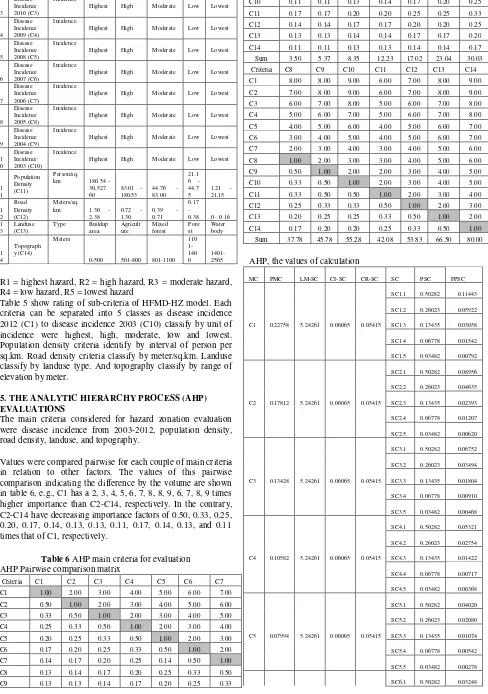
Table 5 show rating of sub-criteria of HFMD-HZ model. Each criteria can be separated into 5 classes as disease incidence 2012 (C1) to disease incidence 2003 (C10) classify by unit of incidence were highest, high, moderate, low and lowest. Population density criteria identify by interval of person per sq.km. Road density criteria classify by meter/sq.km. Landuse classify by landuse type. And topography classify by range of elevation by meter.
5. THE ANALYTIC HIERARCHY PROCESS (AHP) EVALUATIONS
The main criteria considered for hazard zonation evaluation were disease incidence from 2003-2012, population density, road density, landuse, and topography.
Values were compared pairwise for each couple of main criteria in relation to other factors. The values of this pairwise comparison indicating the difference by the volume are shown in table 6, e.g., C1 has a 2, 3, 4, 5, 6, 7, 8, 8, 9, 6, 7, 8, 9 times higher importance than C2-C14, respectively. In the contrary, C2-C14 have decreasing importance factors of 0.50, 0.33, 0.25, 0.20, 0.17, 0.14, 0.13, 0.13, 0.11, 0.17, 0.14, 0.13, and 0.11 times that of C1, respectively.
Table 6 AHP main criteria for evaluation AHP Pairwise comparison matrix
Criteria C1 C2 C3 C4 C5 C6 C7
AHP, the values of calculation
MC PMC LM-SC CI-SC CR-SC SC PSC FPSC
SC6.2 0.26023 0.01681 C6 0.06459 5.24261 0.06065 0.05415 SC6.3 0.13435 0.00868
SC6.4 0.06778 0.00438
SC6.5 0.03482 0.00225
SC7.1 0.50282 0.02393
SC7.2 0.26023 0.01238
C7 0.04759 5.24261 0.06065 0.05415 SC7.3 0.13435 0.00639
SC7.4 0.06778 0.00323
SC7.5 0.03482 0.00166
SC8.1 0.50282 0.02028
SC8.2 0.26023 0.01049
C8 0.04033 5.24261 0.06065 0.05415 SC8.3 0.13435 0.00542
SC8.4 0.06778 0.00273
SC8.5 0.03482 0.00140
SC9.1 0.50282 0.01510
SC9.2 0.26023 0.00782
C9 0.03004 5.24261 0.06065 0.05415 SC9.3 0.13435 0.00404
SC9.4 0.06778 0.00204
SC9.5 0.03482 0.00105
SC10.1 0.50282 0.01327
SC10.2 0.26023 0.00687
C10 0.02640 5.24261 0.06065 0.05415 SC10.3 0.13435 0.00355
SC10.4 0.06778 0.00179
SC10.5 0.03482 0.00092
SC11.1 0.50282 0.01223
SC11.2 0.26023 0.00633
C11 0.02431 5.24261 0.06065 0.05415 SC11.3 0.13435 0.00327
SC11.4 0.06778 0.00165
SC11.5 0.03482 0.00085
SC12.1 0.50282 0.00890
SC12.2 0.26023 0.00460
C12 0.01769 5.24261 0.06065 0.05415 SC12.3 0.13435 0.00238
SC12.4 0.06778 0.00120
SC12.5 0.03482 0.00062
SC13.1 0.50282 0.00661
SC13.2 0.26023 0.00342
C13 0.01314 5.24261 0.06065 0.05415 SC13.3 0.13435 0.00177
SC13.4 0.06778 0.00089
SC13.5 0.03482 0.00046
SC14.1 0.50282 0.00511
SC14.2 0.26023 0.00265
C14 0.01016 5.24261 0.06065 0.05415 SC14.3 0.13435 0.00137
SC14.4 0.06778 0.00069
SC14.5 0.03482 0.00035
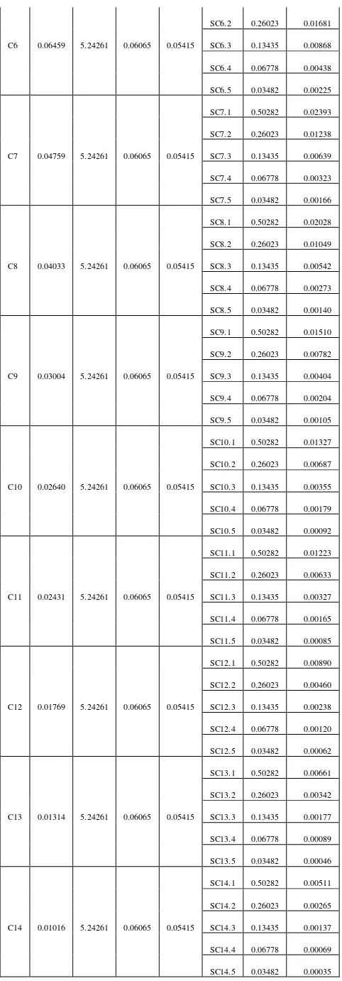
MC = Main Criteria, PMC = Priority of Main Criteria, LM-SC = Lamda max of Sub Criteria, CI-SC = Consistency Index of Sub Criteria, CR-SC = Consistency Ratio of Sub Criteria, SC = Sub Criteria, PSC = Priority of Sub Criteria, FPSC = Final Priority of Sub Criteria, CR-MC = Consistency Ratio of Main Criteria, Lambda max = 15.539468, Consistency index (CI) = 0.118421, Consistency ratio (CR) = 0.075427
The AHP for hazard zonation evaluation resulted in highest importance of weight value of 22.758 % for criteria 1, followed by criteria 2 with a weight value of 17.812 %. The lowest importance weight value of 1.016 % was calculated for criteria 14. For checking accuracy, the consistency ratio (CR) was calculated as 0.075427 which was less than the threshold of 0.1, thus the evaluation was accepted.
Table 7 AHP Sub-criteria pairwise comparison matrix Criteria SC1.1 SC1.2 SC1.3 SC1.4 SC1.5
Priority
Vector PV (%)
SC1.1 1.00 3.00 5.00 7.00 9.00 0.5028 50.28
SC1.2 0.33 1.00 3.00 5.00 7.00 0.2602 26.02
SC1.3 0.20 0.33 1.00 3.00 5.00 0.1344 13.44
SC1.4 0.14 0.20 0.33 1.00 3.00 0.0678 6.78
SC1.5 0.11 0.14 0.20 0.33 1.00 0.0348 3.48
Sum 1.79 4.68 9.53 16.33 25.00 1.0000 100.00
An AHP pairwise comparison matrix was used to evaluate the weighing values of sub-criteria of all 14 main criteria from C1 to C14 in the same way. Table 5.7 shows an example estimation of the sub criteria of the first main criteria. Among C11 through C14, even though the interval contents are different, the values of AHP pairwise comparisons are the same.
Criteria 1 (C1) examined the 5 classes defined by the level of disease incidence. Pairwise values were compared for each pair of classes. The highest disease incidence, sub criteria 1.1, has the highest importance while on the other hand, the lowest disease incidence, sub criteria 1.5, has the least importance.
The calculation by normalized matrix resulted in the highest importance of 50.28% for sub criteria 1.1. The lowest importance value among sub criteria was 3.48 %. The consistency ratio (CR) of 0.05415 indicated an acceptable evaluation.
6. THE FUZZY LOGIC ANALYTIC HIERARCHY PROCESS (FAHP) EVALUATIONS
The evaluation was recalculated applying the fuzzy logic AHP as shown in Table 5.8. The calculation used triangular membership number sets to compare each pair. After a defuzzification process, a normalized matrix was built and the consistency ratio (CR) calculated.
Table 8 FAHP main criteria for evaluation FAHP Pairwise comparison matrix
criteria C1 C2 C3 C4
C1
(1.00,1.00,1.00) (1.00,2.00,3.00) (2.00,3.00,4.00) (3.00,4.00,5.00) C2
(0.33,0.50,1.00) (1.00,1.00,1.00) (1.00,2.00,3.00) (2.00,3.00,4.00) C3
(0.25,0.33,0.50) (0.33,0.50,1.00) (1.00,1.00,1.00) (1.00,2.00,3.00)
C4
(0.20,0.25,0.33) (0.25,0.33,0.50) (0.33,0.50,1.00) (1.00,1.00,1.00) C5
(0.17,0.20,0.25) (0.20,0.25,0.33) (0.25,0.33,0.50) (0.33,0.50,1.00) C6
(0.14,0.17,0.20) (0.17,0.20,0.25) (0.20,0.25,0.33) (0.25,0.33,0.50) C7
(0.13,0.14,0.17) (0.14,0.17,0.20) (0.17,0.20,0.25) (0.20,0.25,0.33) C8
(0.11,0.13,0.14) (0.13,0.14,0.17) (0.14,0.17,0.20) (0.17,0.20,0.25) C9
(0.11,0.13,0.14) (0.11,0.13,0.14) (0.13,0.14,0.17) (0.14,0.17,0.20) C10
(0.11,0.11,0.13) (0.11,0.11,0.13) (0.11,0.13,0.14) (0.13,0.14,0.17) C11
(0.14,0.17,0.20) (0.14,0.17,0.20) (0.17,0.20,0.25) (0.17,0.20,0.25) C12
(0.13,0.14,0.17) (0.13,0.14,0.17) (0.14,0.17,0.20) (0.14,0.17,0.20) C13
(0.11,0.13,0.14) (0.11,0.13,0.14) (0.13,0.14,0.17) (0.13,0.14,0.17) C14
(0.11,0.11,0.13) (0.11,0.11,0.13) (0.11,0.13,0.14) (0.11,0.13,0.14) sum
(3.04,3.50,4.50) (3.93,5.37,7.35) (5.87,8.35,11.35) (8.76,12.23,16.21)
FAHP Pairwise comparison matrix (cont.)
criteria C5 C6 C7 C8
FAHP Pairwise comparison matrix (cont.)
criteria C9 C10 C11
C1
(7.00,8.00,9.00) (8.00,9.00,9.00) (5.00,6.00,7.00) C2 (7.00,8.00,9.00) (8.00,9.00,9.00) (5.00,6.00,7.00)
C3
(6.00,7.00,8.00) (7.00,8.00,9.00) (4.00,5.00,6.00) C4
(5.00,6.00,7.00) (6.00,7.00,8.00) (4.00,5.00,6.00) C5
(4.00,5.00,6.00) (5.00,6.00,7.00) (3.00,4.00,5.00) C6 (3.00,4.00,5.00) (4.00,5.00,6.00) (3.00,4.00,5.00)
C7
(2.00,3.00,4.00) (3.00,4.00,5.00) (2.00,3.00,4.00) C8
(1.00,2.00,3.00) (2.00,3.00,4.00) (2.00,3.00,4.00) C9
(1.00,1.00,1.00) (1.00,2.00,3.00) (1.00,2.00,3.00) C10 (0.33,0.50,1.00) (1.00,1.00,1.00) (1.00,2.00,3.00)
C11
(0.33,0.50,1.00) (0.33,0.50,1.00) (1.00,1.00,1.00) C12
(0.25,0.33,0.50) (0.25,0.33,0.50) (0.33,0.50,1.00) C13
(0.20,0.25,0.33) (0.20,0.25,0.33) (0.25,0.33,0.50) C14
(0.17,0.20,0.25) (0.17,0.20,0.25) (0.20,0.25,0.33) sum
(37.28,45.78,55.08) (45.95,55.28,63.08) (31.78,42.08,52.83)
FAHP Pairwise comparison matrix (cont.)
criter
ia C12 C13 C14
priority vector C1
(6.00,7.00,8.00) (7.00,8.00,9.00) (8.00,9.00,9.00) 0.23864 C2
(6.00,7.00,8.00) (7.00,8.00,9.00) (8.00,9.00,9.00) 0.18839 C3 (5.00,6.00,7.00) (6.00,7.00,8.00) (7.00,8.00,9.00) 0.14290
C4
(5.00,6.00,7.00) (6.00,7.00,8.00) (7.00,8.00,9.00) 0.11239 C5
(4.00,5.00,6.00) (5.00,6.00,7.00) (6.00,7.00,8.00) 0.08485 C6
(4.00,5.00,6.00) (5.00,6.00,7.00) (6.00,7.00,8.00) 0.06838 C7 (3.00,4.00,5.00) (4.00,5.00,6.00) (5.00,6.00,7.00) 0.05127
C8
(3.00,4.00,5.00) (4.00,5.00,6.00) (5.00,6.00,7.00) 0.04266 C9
(2.00,3.00,4.00) (3.00,4.00,5.00) (4.00,5.00,6.00) 0.03185 C10
(2.00,3.00,4.00) (3.00,4.00,5.00) (4.00,5.00,6.00) 0.02800 C11 (1.00,2.00,3.00) (2.00,3.00,4.00) (3.00,4.00,5.00) 0.02603
C12
(1.00,1.00,1.00) (1.00,2.00,3.00) (2.00,3.00,4.00) 0.01886 C13
(0.33,0.50,1.00) (1.00,1.00,1.00) (1.00,2.00,3.00) 0.01395 C14
(0.25,0.33,0.50) (0.33,0.50,1.00) (1.00,1.00,1.00) 0.01081 sum (42.58,53.83,65. Road density, C13= Landuse, C14= Topography
FAHP, the value of calculation
MC PMC LM-SC CI-SC CR-SC SC PSC FPSC
SC4.1 0.50004 0.05314
SC4.2 0.26149 0.02779
C4 0.10626 5.29212 0.07303 0.06521 SC4.3 0.13518 0.01436
SC4.4 0.06823 0.00725
SC4.5 0.03507 0.00373
SC5.1 0.50004 0.04017
SC5.2 0.26149 0.02100
C5 0.08033 5.29212 0.07303 0.06521 SC5.3 0.13518 0.01086
SC5.4 0.06823 0.00548
SC5.5 0.03507 0.00282
SC6.1 0.50004 0.03245
SC6.2 0.26149 0.01697
C6 0.06490 5.29212 0.07303 0.06521 SC6.3 0.13518 0.00877
SC6.4 0.06823 0.00443
SC6.5 0.03507 0.00228
SC7.1 0.50004 0.02432
SC7.2 0.26149 0.01272
C7 0.04863 5.29212 0.07303 0.06521 SC7.3 0.13518 0.00657
SC7.4 0.06823 0.00332
SC7.5 0.03507 0.00171
SC8.1 0.50004 0.02026
SC8.2 0.26149 0.01059
C8 0.04051 5.29212 0.07303 0.06521 SC8.3 0.13518 0.00548
SC8.4 0.06823 0.00276
SC8.5 0.03507 0.00142
SC9.1 0.50004 0.01509
SC9.2 0.26149 0.00789
C9 0.03017 5.29212 0.07303 0.06521 SC9.3 0.13518 0.00408
SC9.4 0.06823 0.00206
SC9.5 0.03507 0.00106
SC10.1 0.50004 0.01329
SC10.2 0.26149 0.00695
C10 0.02659 5.29212 0.07303 0.06521 SC10.3 0.13518 0.00359
SC10.4 0.06823 0.00181
SC10.5 0.03507 0.00093
SC11.1 0.50004 0.01230
SC11.2 0.26149 0.00643
C11 0.02460 5.29212 0.07303 0.06521 SC11.3 0.13518 0.00333
SC11.4 0.06823 0.00168
SC11.5 0.03507 0.00086
SC12.1 0.50004 0.00892
SC12.2 0.26149 0.00467
C12 0.01784 5.29212 0.07303 0.06521 SC12.3 0.13518 0.00241
SC12.4 0.06823 0.00122
SC12.5 0.03507 0.00063
SC13.1 0.50004 0.00661
SC13.2 0.26149 0.00346
C13 0.01322 5.29212 0.07303 0.06521 SC13.3 0.13518 0.00179
SC13.4 0.06823 0.00090
SC13.5 0.03507 0.00046
SC14.1 0.50004 0.00515
SC14.2 0.26149 0.00269
C14 0.01030 5.29212 0.07303 0.06521 SC14.3 0.13518 0.00139
SC14.4 0.06823 0.00070
SC14.5 0.03507 0.00036
MC = Main Criteria, PMC = Priority of Main Criteria, LM-SC = Lamda max of Sub Criteria, CI-SC = Consistency Index of Sub Criteria, CR-SC = Consistency Ratio of Sub Criteria, SC = Sub Criteria, PSC = Priority of Sub Criteria, FPSC = Final Priority of Sub Criteria, CR-MC = Consistency Ratio of Main Criteria, Lambda max = 15.886626, Consistency index (CI) = 0.145125, Consistency ratio (CR) = 0.092436, Consistency Ratio is less than 0.1. Therefore, this evaluation is acceptable.
The achieved weight of each criteria as analyzed by Fuzzy AHP is shown in Table 5.8. This table represents the highest weight value as Criteria 1 (disease incidence 2012) with 22.437 %. The second highest weight value was attributed to Criteria 2 (disease incidence 2011) with 17.756 %, while Criteria 14, topography, had the least weight value of 1.030 %.
Table 9 FAHP pairwise comparison of sub-criteria
Criteria SC1.1 SC1.2 SC1.3 SC1.4 SC1.5
SC1.1 (1.00, 1.00, 1.00)
(2.00, 3.00, 4.00)
(4.00, 5.00, 6.00)
(6.00, 7.00, 8.00)
(8.00, 9.00, 9.00)
SC1.2 (0.25, 0.33, 0.50)
(1.00, 1.00, 1.00)
(2.00, 3.00, 4.00)
(4.00, 5.00, 6.00)
(6.00, 7.00, 8.00)
SC1.3 (0.17, 0.20, 0.25)
(0.25, 0.33, 0.50)
(1.00, 1.00, 1.00)
(2.00, 3.00, 4.00)
(4.00, 5.00, 6.00)
SC1.4 (0.13, 0.14, 0.17)
(0.17, 0.20, 0.25)
(0.25, 0.33, 0.50)
(1.00, 1.00, 1.00)
(2.00, 3.00, 4.00)
SC1.5 (0.11, 0.11, 0.13)
(0.13, 0.14, 0.17)
(0.17, 0.20, 0.25)
(0.25, 0.33, 0.50)
(1.00, 1.00, 1.00)
sum (1.65, 1.79, 2.04)
(3.54, 4.68, 5.92)
(7.42, 9.53, 11.75)
(13.25, 16.33, 19.50)
(21.00, 25.00, 28.00)
SC1.1=highest incidence, SC1.2=high incidence, SC1.3=moderate incidence, SC1.4=low incidence, SC1.5=lowest incidence
An FAHP pairwise comparison matrix was used to evaluate the weighing values of sub-criteria of all 14 main criteria from C1 to C14 in the same way. Table 5.9 shows an example calculation of the sub criteria of the first main criteria. With a value of 0.06521, the CR was lower than 0.1. Therefore, the evaluation was accepted.
Again, Criteria 1 (C1) examined the 5 classes defined by the level of disease incidence. Pairwise values were compared for each pair of classes. The highest disease incidence, sub criteria 1.1, has the highest importance while on the other hand, the
lowest disease incidence, sub criteria 1.5, has the least importance.
Figure 7 Final priority value of AHP and FAHP approach
Figure 7 shows the final priority values of each sub-criteria of the 14 main criteria as calculated by both AHP and FAHP approaches. It can be seen that FAHP figures are always higher than AHP figures. The numbers decrease systematically from criteria 1 (C1) to criteria 14 (C14).
7. RESULTS
7.1 The HFMD-HZ model
The HFMD-HZ map was established using a WLC method. WLC is most often used to monitor spatial multi-attribute decision making. It can be used to generate a risk map with various zones and to measure the weightings factors (Rakotomanana et al., 2007). WLC is a combination method that describes how different factors equilibrium each other and specifies their relative importance (Gorsevski et. al., 2012). The weight value is calculated by multiplying the main criteria with sub criteria of the same hierarchical classes and summarizing the result over all attributes to produce a total weight score by equation (24). Then, an HFMD-HZ map is generated as a single resulting layer by the calculation shown in equation (25)
k k iki
w
r
R
(24)Where, wk andrik are vectors of priorities of the main and sub-criteria, respectively.
(25)
Where; C is factor weight of 14 factors: C1= Inc 2012, C2=Inc
2011, C3=Inc 2010, C4=Inc 2009, C5=Inc 2008, C6=Inc 2007, C7=Inc 2006, C8=Inc 2005, C9=Inc 2004, C10=Inc 2003, C11= Population density, C12= Road density, C13= Landuse, C14= Topography
Wi is the weight of sub-criteria.
Wm is the weight of main criteria
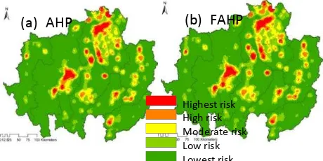
Figure 8 The result of AHP and Fuzzy AHP analysis approach
The resulting HFMD-HZ model generated by AHP approach shows the 5 classes: Highest risk, high risk, moderate risk, low risk and lowest risk. Highest risk areas appear in many places, with the most prominent within two provinces, one in the central area of Chiang Mai province, the second in Chiang Rai province. Others were minor, e.g. in Phayao province, mainly on the west side; in Lampang province in northern part; in Nan in the top north and south parts of province; in the central area of Phrae province; in the southern region of Uttaradit province; and a small area in the southern part of Mae Hong Son province (Figure 8 (a)). The highest risk area covered 3,308.39 sqkm or 2.48% of the study area (Table 10), followed by high risk areas with 3,786.44 sqkm or4.07% of the study area. The moderate risk area near the buffer zone between highest and high risk areas came in third. Moderate risk areas had 8,330.91 sqkm (8.95%). Low risk areas mainly appeared in the center of Chiang Mai - Lamphun, Chiang Rai - Phayao and the center of Lampang accounting for 13,352 sqkm or 14.35%. Lowest risk areas were found in all provinces covering 70.1%or65,251.62 sqkm.
The results of the model created by FAHP approach (Figure 8 (b)) were overall found to be similar to those of the AHP approach. Highest risk areas (R1) appear in 2 groups at Chiang Mai and Chiang Rai province, covering the smallest share. By contrast, the lowest risk area (R5) made up the largest part of the whole area. In detail, the highest risk zone had 2,385.98 sqkm or 2.56 % of the whole area. The high risk area had 3985.310911sqkm or 4.283893 %. The lowest risk area made up 64,896.378109 sqkm or 69.758452 %.
Table 10 Area of hazard zonation map
Risk
AHP FAHP
area
(sq.km.) %
area
(sq.km.) %
Highest
(R1) 2308.39 2.48 2385.98 2.56
High
(R2) 3786.44 4.07 3985.31 4.28
Moderate
(R3) 8330.91 8.95 8365.29 8.99
Low
(R4) 13352.74 14.35 13397.15 14.40
Lowest
(R5) 65251.62 70.14 64896.37 69.75
total 93030.12 100.00 93030.12 100.00
HZ
I
C
1W
iC
2W
iC
3W
i...
HFMD
(a)
AHP
AHP_C1
0.0 0.0 0.0 0.0 0.0
Highest risk High risk Moderate risk Low risk Lowest risk
(b)
FAHP
...
C
14W
i/
Wm
7.2 The model validation
The data used to check the results were actual data of disease incidence in 2013 (Figure 9). In general, the pattern was found to be very similar to the results of both AHP and FAHP models. The highest risk area can be seen at the top of study area within Chiang Rai province. High risk areas can be seen mostly in populated areas in Chiang Mai, Phayao, Lampang Phrae and Nan provinces. In 2013, the least risk zone were found in the west and the south of the study area.
Figure 9 The validate data (disease incidence in 2013)
Table 11 AHP validation
AHP
Rahp-1 Rahp-2 Rahp-3
sq.km % sq.km % sq.km %
VR1 378.2 0.4 47.5 0.0 35.1 0.0
VR2 649.1 0.7 528.7 0.5 213.0 0.2
VR3 810.0 0.8 1067.8 1.1 2036.5 2.1
VR4 311.4 0.3 1173.1 1.2 3097.8 3.3
VR5 159.5 0.1 969.1 1.0 2948.3 3.1
total 2308.4 2.4 3786.4 4.0 8330.9 8.9
AHP
Rahp-4 Rahp-5 Total
sq.km % sq.km % sq.km %
VR1 7.9 0.0 0.6 0.0 469.5 0.5
VR2 128.3 0.1 174.1 0.1 1693.4 1.8
VR3 1471.9 1.5 1123.5 1.2 6509.8 7.0
VR4 4929.3 5.3 6401.3 6.8 15913.0 17.1
VR5 6815.1 7.3 57551.9 61.8 68444.1 73.5
total 13352.7 14.3 65251.6 70.1 93030.1 100.0
Rahp-1 = AHP highest risk, Rahp-2 = AHP high risk, Rahp-3 = AHP moderate risk, Rahp-4 = AHP low risk, Rahp-5 = AHP lowest risk, VR1 = Validate data highest risk, VR2 = Validate data high risk, VR3 = Validate data moderate risk, VR4 = Validate data low risk, VR5 = Validate data lowest risk
Table 12 FAHP validation
FAHP
Rfahp-1 Rfahp-2 Rfahp-3
sq.km % sq.km % sq.km %
VR1 379.7 0.4 46.8 0.0 34.3 0.0
VR2 676.4 0.7 509.1 0.5 211.1 0.2
VR3 828.1 0.8 1115.3 1.2 2051.6 2.2
VR4 322.9 0.3 1249.1 1.3 3102.4 3.3
VR5 178.6 0.1 1064.8 1.1 2965.6 3.1
total 2385.9 2.5 3985.3 4.2 8365.2 8.9
FAHP
Rfahp-4 Rfahp-5 Total
sq.km % sq.km % sq.km %
VR1 7.9 0.0 0.5 0.0 469.5 0.5
VR2 137.2 0.1 159.4 0.1 1693.4 1.8
VR3 1401.6 1.5 1113.1 1.2 6509.8 7.0
VR4 4937.6 5.3 6300.8 6.7 15913.0 17.1
VR5 6912.6 7.4 57322.4 61.6 68444.1 73.5
total 13397.1 14.4 64896.3 69.7 93030.1 100.0
Rfahp-1 = FAHP highest risk, Rfahp-2 = FAHP high risk, Rfahp-3 = FAHP moderate risk, Rfahp-4 = FAHP low risk, Rfahp-5 = FAHP lowest risk, VR1 = Validate data highest risk, VR2 = Validate data high risk, VR3 = Validate data moderate risk, VR4 = Validate data low risk, VR5 = Validate data lowest risk
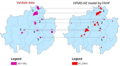
Tables 11 and 12 show the accuracy check of the results of the HFMD-HZ models created by AHP and FAHP approaches by spatial validation. The FAHP approach was found to be more accurate with a good match, particularly of the highest risk area located in the top northern area of Chiang Rai. While the high risk areas shown by the AHP model were a better match, moderate, low and lowest risk areas calculated by FAHP were more accurate than those of AHP.
Table 13 Comparison between AHP and FAHP validation (area matching)
risk
R1 R2 R3
AHP FAHP AHP FAHP AHP FAHP
VR1 80.55 80.86 10.12 9.98 7.47 7.32
VR2 38.33 39.94 31.22 30.06 12.58 12.47
VR3 12.44 12.72 16.40 17.13 31.28 31.51
VR4 1.95 2.03 7.37 7.85 19.46 19.49
VR5 0.23 0.26 1.41 1.55 4.30 4.33
total 2.48 2.56 4.07 4.28 8.95 8.99
risk
R4 R5 Total
AHP FAHP AHP FAHP AHP FAHP
VR1 1.68 1.70 0.14 0.11 469.56 0.50
VR2 7.58 8.10 10.28 9.41 1693.48 1.82
VR3 22.61 21.53 17.25 17.09 6509.88 7.00
VR4 30.97 31.02 40.22 39.59 15913.07 17.11
VR5 9.95 10.10 84.08 83.75 68444.14 73.57
total 14.35 14.40 70.14 69.75 93030.13 100.00
Table 13 shows the matrix table of the model analysis containing the relations between AHP and FAHP results with validation data for every class pair as follows: R1 with VR1, R2 with VR2, R3 with VR3, R4 with VR4, R5 with VR5.
The highest risk areas (R1) of AHP and FAHP were 80.558 % and 80.869% consistent with validation data, respectively, high risk areas (R2) at 31.224%, 30.065 %, moderate risk areas (R3)
AHP_C1 0.0 0.0 0.0 0.0 0.0
Highest risk High risk Moderate risk Low risk Lowest risk
at 31.284%, 31.515%, low risk areas (R4) at 30.977%, 31,029%, and lowest risk areas (R5) at 84.086%, 83.751% respectively. Concluding, it is to be noted that FAHP achieved higher consistency than AHP in R1, R3, R5 classes while in R2 and R4 classes, AHP results were more consistent than FAHP results.
8. DISCUSSIONS
When classes 1 and 2 were combined, the spatial pattern was found to be more consistent, particularly, the HFMD-HZ model created by the FAHP approach. Figure 10 shows the spatial pattern of the 7 areas with the highest outbreak risk in 5 provinces: Chiang Rai, Phayao, Chiang Mai, Lampang and Phrae. The result of the FAHP model proved more consistent than the AHP result.
Figure 10 Seven groups inside five province are highest hazard outbreak
Although the outbreak prediction model could not make exact predictions, it could at least demonstrate its usefulness for control or prevention measures before any disease outbreak by estimating the trend in the area.
Table 14 presents the highest risk areas (R1) as calculated by AHP and FAHP for each province. The largest share was found in Chiang Rai with 41.10 % of the total R1 area (most of it in Muang district with 407 sq.km.) followed by Chiang Mai with 26.48 %, most of it in Sankampang district, Phayao with 10.78 %, and Lampang province with 9.72 %. Mae Hong Son province had the smallest R1 risk area with 25.18 sq.km. or 1.06% of whole R1 area.
Table 14 The highest hazard area (R1) by FAHP
Province R1_FAHP
(sq.km.)
FAHP %
District
1. Chiang
Rai 980.56 41.10
Muang, Wiang, Chiangrung, Chiangsan, Wiang Chai, Maesai, Maeloa, Wiang, Papao, Maejan, Doiluang 2.
Chiang Mai
631.80
26.48
Sankampang, Mueang, Jomtong, Samsai, Hangdong, Doi Saket, Saraphi, Maerim, Sampatong, Doiloh, Maeey, Phang 3.
Phayao 257.22 10.78
Muang, Chiang kam, Mae jai, Pong, Phusang
4. 231.96 9.72 Muangpan, Wangnue,
Lampang Ngow, Hangchat, Jaehom
5.
Lamphun 90.00 3.77
Phasang, Wiang Nonglong, Banhong, Muang
6. Phrae 62.44 2.62 Rongkwong, Nong
Mungkai, Muang
7. Nan 59.83 2.51 Tungchang, Na muan,
Chiangkrang, Pua 8.
Uttaradit 46.99 1.97
Muang, Lablae
9. Mae Hong
Son 25.18
1.06
Muang
Total 2385.98 100.00
Figure 11 Kindergarten site and its located at the highest zone of HFMD-HZ model
Figure 11 shows an analysis by an overlay of the highest risk areas (R1) and kindergarten sites. The results show the kindergarten sites where maximum surveillance should be provided in two area groups, one in Muang Chiang Mai district with 54 sites and another in Muang Chiang Rai district with 17 sites. Other minor kindergarten sites that should be included in maximum surveillance were found in Phayao, Lampang and Uttaradit provinces.
9. CONCLUSION
HFMD trends to intensify in both the patient number and mutations of the virus. Attempts to better understand the spatial nature of outbreaks can be useful for surveillance and prevention measures before any outbreak occurs. This research investigated the application of GIS with multi criteria decision analysis (MCDA) by AHP and Fuzzy logic of triangular number sets due to its ability to take into account both quantitative and qualitative measures. Northern Thailand was chosen as study area for the generation of a Hand, Foot and Mouth Disease Hazard Zonation (HFMD-HZ) model because it is the area with the most HFMD outbreaks over 10 years (Samphutthanon R., et. al., 2014). Spatial factors considered were 3 main criteria in descending order of importance as follows: disease incidence, socio-economic and physical features. These were divided into 14 sub criteria. The AHP calculations showed a consistency ratio (CR) value of 0.075427, while the CR of the FAHP calculation approach was 0.092436. Both figures were below the threshold of 0.1, which means the evaluations were accepted. The final priority value of the FAHP approach was greater than that of AHP for all sub criteria.
! L
R1
Kindergarten
Highest risk by FAHP Kindergarten
R
Linking to geospatial data by using GIS and Weighted Linear Combination (WLC) to create a hazard zonation map, spatial patterns appeared quite similar to those of the actual data (spatial incidence 2013), which proved that the results were satisfying. Going into more detail, the FAHP approach was found to be more accurate than AHP, particularly concerning highest risk and high risk areas (Chiang Rai, Phayao, Chiang Mai, Lampang and Phrae). The overlay with kindergarten sites showed 2 main areal groups where special surveillance was indicated in the area of Mueang District of Chiang Mai and Mueang District of Chiang Rai provinces. This may be useful for planning preventive measures against HFMD outbreaks by concerned agencies.
Finally, it can be concluded that the integration of GIS with a Fuzzy logic AHP approach is capable of providing satisfactory results in predicting HFMD outbreaks in the study area. Another factor that should be considered together with surveillance is the temporal pattern of outbreaks.
ACKNOWLEDGMENTS
We would like to thank the Bureau of Epidemiology, Ministry of Public Health, Department of Provincial Administration, Ministry of Interior of Thailand, Department of Highways, Ministry of Transportation of Thailand, Land Development Department, Ministry of Agriculture and Cooperatives of Thailand and Geo-Informatics and the Space Technology Development Agency, Ministry of Science and Technology of Thailand for providing invaluable information.
REFERENCES
Banai R., "Fuzziness in geographic information systems: contributions from the analytic hierarchy process "International Journal of Geographical Information Systems. 1993, vol.7, pp. 315–329.
Boroushaki S, Malczewski J. Implementing an extension of the analytical hierarchy process using ordered weighted averaging operators with fuzzy quantifiers in ArcGIS. Comput.Geosci. 2008, 34: 399-410.
Chang, D. Y., Applications of the extent analysis method on fuzzy AHP. European Journal of Operational Research. 1996, 95(3), 649-655.
Cheng C.H., Yang K.L., and Hwang C.L., "Evaluating attack helicopters by AHP based on linguistic variable weight "European Journal of Operational Research. 1999, vol.116, pp. 423-435.
Eastman J.R., "Idrisi for Windows, Version 2.0: Tutorial Exercises ", Graduate School of Geography-Clark University, Worcester, MA, 1997.
Farkas A., "Route/Site Selection of Urban Transportation Facilities: An Integrated GIS/MCDM Approach", In Proceedings of the 7th International Conference on Management, Enterprise and Benchmarking, June 5-6, Budapest, and Hungary. 2009, pp.169-184.
Gorsevski, P.V.,et al., Integrating multi-criteria evaluation techniques with geographic information systems for landfill site selection: a case study using ordered weighted average. Waste Management. 2012, 32, 287–296.
Gumus, A. T., Evaluation of hazardous waste transportation firms by using a two step fuzzy-AHP and TOPSIS methodology. Expert Systems with Applications. 2009, 36(2), 4067-4074.
Kordi, M., & Brandt, S.A., Effects of increasing fuzziness on analytic hierarchy process for spatial multicriteria decision analysis. Computers, Environment and Urban Systems. 2012, 36(1), 43–53. doi:10.1016/j.compenvurbsys.2011.07.004.
Malczewski J., "GIS based land use suitability analysis: a critical overview" Progress in Planning. 2004, vol. 62 (1), pp. 3–65.
Malczewski J., "GIS-based multicriteria decision analysis: a survey of the literature" International Journal of Geographical Information Science. 2006, vol. 20 pp.703–726.
Malczewski J., GIS and Multicriteria Desision Analysis, New York: John Willey and Sons, Inc. 1999, p. 395.
Mikhailov L., Deriving priorities from fuzzy pairwise comparison judgments. Fuzzy Set. Syst., 2003, 134: 365-385.
Nobre, F.F., Trotta, L.T.F., Gomes, L.F.A.M., Multicriteria decision making: An approach to setting priorities in health care. Symposium on statistical bases for public health decision making: from exploration to modeling. 1999, 18(23), pp. 3345 – 3354.
Rakotomanana, F.; Randremanana, R.V.; Rabarijaona, L.P.; Duchemin, J.B.; Ratovonjato, J.; Ariey, F. Determining areas that require indoor insecticide spraying using multi-criteria evaluation, a decision-support tool for malaria vector control programmes in the Central highlands of Madagascar. International Journal of Health Geographics. 2007, 6, 1-11.
Saaty L.T., The Analytic Hierarchy Process, McGraw-Hill, New York 1980.
Saaty L.T., The Analytic Hierarchy Process: Planning, Priority Setting, Resource Allocation, New York, McGraw-Hill International. 1980, p 437.
Samphutthanon, R.; Tripathi, N.K.; Ninsawat, S.; Duboz, R. Spatio-Temporal Distribution and Hotspots of Hand, Foot and Mouth Disease (HFMD) in Northern Thailand. Int. J. Environ. Res. Public Health. 2014, 11, 312-336.
Steinitz, C., Parker, P., & Jordan, L., Hand drawn overlays: their history and prospective uses. Landscape Architecture. 1976, 9, 444-455.
Vahidnia M.H., Alesheikh A., Alimohammadi A., Bassiri A. , "Fuzzy analytical hierarchy process in GIS application" The International Archives of the Photogrammetry, Remote Sensing and Spatial Information Sciences, Beijing. 2008, vol. 37 pp. 593-596.
Zadeh LA., Fuzzy sets. Inf. Control. 1965, 8: 338-353.
Ziaei, M., Hajizade, F., Fuzzy analytical hierarchy process (FAHP): a GIS-based multicriteria evaluation/selection analysis. 19th International Conference on Geoinformatics. 2011, 19 (11), 1–6, 24–26.