An assessment of the spatial variability of basal area
in a terrain covered by Mediterranean woodlands
Raymond Salvador
a,b,∗,1aSpace Applications Institute, Joint Research Centre TP950, I-21020 Ispra (Va), Italy
bCentre de Recerca Ecològica i Aplicacions Forestals, Universitat Autònoma de Barcelona, 08193 Bellaterra, Barcelona, Spain
Received 14 July 1999; received in revised form 22 December 1999; accepted 21 February 2000
Abstract
Spatial patterns of Mediterranean woodlands are largely unknown. An exploratory analysis of the spatial structure of basal area was carried out in this type of community. Specifically, an area of non-disturbed woodlands located in the north-east of the Iberian peninsula was analysed. Direct and indirect evidences for the hypothesis stating that environmental factors lead to the establishment of spatial patterns on the basal area of non-disturbed Mediterranean woodlands were investigated. The results showed that the variability of this parameter occurs within really short spatial intervals (of less than 100 m) and neither radiation nor the slope seemed to have an important effect on it. In consequence, results did not support the previously mentioned hypothesis. Among others, long term effects of forest management, an uneven presence of relief conditions and a complex dynamics of basal area within plots were suggested as explanations for the results found. Finally, some recommendations and practical advises were set for future inventories and studies of spatial patterns in Mediterranean woodlands. © 2000 Elsevier Science B.V. All rights reserved.
Keywords: Mediterranean woodlands; Spatial autocorrelation; Basal area; Solar radiation; Slope
1. Introduction
Although Mediterranean woodlands are affected by diverse biotic and abiotic factors, human activities may have significant effects modifying their dynamics and the ruling power of such factors on their final struc-ture. In addition, the frequent wildfires occurring in Mediterranean areas, sometimes due to natural causes, have important consequences over woodlands. They
∗Tel.:+34-93-5812666; fax:+34-93-5811312. E-mail address: [email protected] (R. Salvador)
1Information regarding this manuscript should be sent to second
address.
break the growing process of individuals, attenuate the ruling capacity of biotic and abiotic agents in the late stages of woodland dynamics and often increase the heterogeneity of landscapes.
Yet, some specific areas with special interest have been preserved for many years avoiding human in-tervention and the occurrence of wildfires. In these cases it might be expected for the biotic and abiotic factors to affect significantly the structure of Mediter-ranean woodlands. For instance, since abiotic factors such as radiation and the slope are directly related to water availability in plants and to soil properties, they will probably have a noticeable effect (Hellmers et al., 1955; Oechel et al., 1981; Spetch, 1988; Mayor and
Rodà, 1994), but the less known biotic agents, such as the dispersion processes, may be also significant (Herrera et al., 1994).
Clearly, these factors will not act in an independent way in the different sites of a forest but will create spatial patterns in its structure. In order to deal with the analysis of the spatial distribution of variables a number of statistical tools have been developed (see Legendre and Fortin (1989) for an applied review). These tools usually quantify the spatial autocorre-lation, which is the degree of similarity (or dissim-ilarity) between points due to their relative spatial location (Cliff and Ord, 1981). Several autocorrela-tion coefficients have been defined to estimate the degree of resemblance of point values located at a specific distance apart from each other. In addition to the study of the original data, there is also the chance to check for the presence of spatial autocorrelation in residual values (after considering the effect of other variables through a linear model) or to build a more complex model containing an autoregressive structure (Cliff and Ord, 1981; Ripley, 1981).
The development of geographical information sys-tems (GIS) in recent years allows an easier manage-ment of geolocated data (Burrough and McDonnell, 1998). Specifically, data coming from various layers of information may be derived and combined with point data sampled in the field to carry out further analyses. For instance, some of the previously men-tioned variables, such as radiation and slope, may be obtained from digital elevation models (DEMs) and analysed together with woodland structural param-eters derived from forest surveys. Due to its direct relation to biomass and to its easy collection, basal area (BA) is one of the most suitable parameters to describe the structure of woodlands. Although BA is species and succession stage dependent it can be hypothesised that, within uneven stands of mixed species left growing freely for a large period of time, environmental variables will shape its spatial patterns.
The primary objective of this study was the ex-ploratory analysis of the spatial structure of BA in a terrain covered by Mediterranean woodlands, which have not been affected by timbering or wildfires for a long period of time. Direct and indirect evidences for the hypothesis stating that environmental factors lead to the establishment of spatial patterns on the
BA of non-disturbed Mediterranean woodlands were investigated.
2. Methodology
2.1. The study area and the field information available
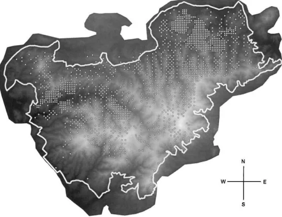
This study was carried out with different data deri-ved from the Parc de Collserola, a protected woodland area beside the city of Barcelona, on the northeast-ern coast of Spain. It has an extension of 8465 ha with a rather mountainous relief (Fig. 1). Altitudes range from 100 to 512 m with a typical Mediterranean climate (annual mean precipitation of 504 mm and monthly mean temperatures ranging from 8.8◦C in January to 23.7◦C in July) with high levels of water deficit during summer. The main large woody species belong to the genus Quercus and Pinus, but other Mediterranean shrubs are also abundant. This vegeta-tion grows above lithological strata predominantly of shales and granite but limestone is also present in a few places.
Last intensive extraction of timber in the study area occurred just after the Spanish civil war (1936–1939), and a demographic study (Canadell and Irizar, 1988) points to a period of, at least, 50 years with no inter-vention until the present day (with the exception of timber extraction in few local areas). Thus, woodlands have grown freely achieving a clearly uneven-aged structure. This process has been supported by an ef-fective fire suppression program avoiding significant wildfires in all the study area except the south-facing slope next to the city of Barcelona.
Fig. 1. Digital elevation model, limits of the study area and location of the 1520 field plots used.
The joint BA values for each plot were used to analyse the global effect of factors and levels of vari-ability described in Section 2.2 below. Separate BA values were also used for the five woody species most frequently found in the study area: Quercus ilex L. (present in 1440 plots), Pinus halepensis Mill. (in 1382 plots), Quercus cerrioides Wk. (in 1146 plots),
Arbutus unedo L. (in 603 plots) and Pinus pinea L.
(in 207 plots). Although, the BA of any one species in a mixture was dependent on the BA of other species present, the analysis of each species separately de-termined the net effect (on individual species) of the factors and levels of spatial variability studied.
2.2. Three levels of spatial variability
As suggested in the introduction, various biotic and abiotic factors were probably affecting the spatial dis-tribution of the BA in the study area. However, a sep-arate examination of each of them was beyond the scope of this work and more general procedures were applied to study the BA spatial structure. Specifically, two criteria were used to select the analyses to be car-ried out: (1) the information of the study area available in a direct or indirect way, and (2) the expected ability of the analyses to explain the spatial patterns of BA.
Following both criteria, the study of the spatial pat-terns of BA was summarised in three different analyses directly related to three distinct levels of spatial vari-ability. These are described in the following sections.
2.2.1. The regional level variability
This level is concerned with medium and large scale variations such as environmental gradients. Many of them are caused by gradual modifications in the mean meteorological conditions (e.g. the latitudinal gradi-ents or the gradigradi-ents due to distance from the sea). Obviously, since big areas are more likely to be af-fected by this type of variability, it was not expected that such gradients would explain the greater part of the variance observed in the BA in the study area (although coastal regions may be more prone to strong environmental variations).
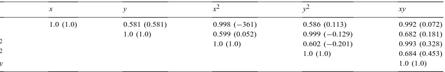
Table 1
Matrix of correlation coefficients found between the independent variables to be used in the trend surface analysis, before and after their re-scalinga,b
aUTM coordinates of all field plots (n=1520) were used. bValues re-scaled are given in parenthesis.
(x2, y2) and their cross-products (xy) were tried as independent variables for all species except P. pinea. In this species, only the original x, y coordinates were used in order to avoid the possibility of fitting spurious models as a consequence of a much lower number of available plots.
The inclusion of original and squared values of the same variable in a model frequently leads to ma-trix collinearity problems (Rawlings et al., 1998). Since full UTM coordinates were initially used (i.e. large and positive numbers) very high correlations were found between some of the derived indepen-dent variables (see Table 1). Following Peña (1989) the original UTM coordinates were re-scaled by sub-traction of their mean value, obtaining much lower correlations (Table 1). This same process linked the minimum absolute values for x2, y2 and xy to the new origin of coordinates located close to the central part of the study area, allowing an easier in-terpretation of significant coefficients as differences between the central region and the boundaries of the study area.
2.2.2. The set of physical variables related to relief
A digital elevation model (DEM) of the study area was available with a high grid resolution of 5 m. From all the variables possibly derived from a DEM, two of them were chosen as they would probably affect the structure of woodlands in a significant way: the slope and the mean value of the daily potential solar radia-tion for the whole year over each plot. This last param-eter was regarded as potential since it does not con-sider the presence of clouds. However, being a small area, large spatial differences in mean cloudiness were not expected and potential values were considered as nearly proportional to the real ones.
The retrieval of slopes was directly carried out by choosing the maximum weighted differences in height values of neighbour grid points (Burrough and Mc-Donnell, 1998). Data were given in degrees (range 0–90). The calculation of the mean value of the daily potential solar radiation for the whole year took into account the sun elevation angle, the slope, the aspect and the indirect shadowing produced by the surround-ing mountains (Pons, 1996). Radiation data were given in units of 106J m−2mm−1. In order to obtain reliable
values of both variables and to minimise sample noise, mean values from 5×5 pixel windows centred in the plot coordinates were given for each one of the field plots.
The two variables selected were probably related, in an indirect way, with other variables that may also have a significant influence over the structure of wood-lands, but which required complicated and irksome measurements (such as the soil depth, the soil water content or the real radiation). Therefore, if there were a consistent effect of these variables over the BA, some statistical significance in the variables analysed would be expected.
Linear regression was again selected to model the effect of radiation and slope on the BA values. Indeed, to integrate factors in a single model, both variables were considered in the fitting of the trend surface analysis of the previous subsection. This was carried out by a stepwise variable selection method (Rawlings et al., 1998). Starting with models in-cluding all possible independent variables (x, y, x2,
y2, xy, radiation and slope) less informing variables were sequentially dropped as these led to the low-est value of the Cp statistic (until the elimination of
any variable could not lower the Cp of the previous
Mont-gomery and Peck (1992) for a description of the Cp
statistic.
2.2.3. The autocorrelation at the local level
There are many statistics available to quantify the autocorrelation within a sample. One of the most com-monly used is the Moran autocorrelation coefficient, which is defined by Cliff and Ord (1981) as:
I = n
where n is the total number of plots, wij the geo-graphical connection between plot i and plot j (usu-ally given as the reciprocal of a simple function of the distance), and zi is the value of the studied variable (BA) in plot i, after re-scaling through the subtraction of the sample mean. The st parameter is the addition
of allwij values, and although usually (but not nec-essarily)wij=wj i, eachwij with a different subscript (so, ij6=ji) is considered as a single value to be
in-cluded in the addition). Furthermore, one plot cannot be connected to itself (wii=0).
An intuitive idea of the information given by I can be easily gained by considering separately the lower and upper sums as
where S1 can be clearly identified as a sample variance (i.e. the mean value of the squared differences to the sample mean). Hence, it provides information about the average variability of the sample. The parameter
S2 is similar to a sample covariance that only considers
the pairs of points with some connection (wij>0). So, it gives the average covariability of values of plots connected. Consequently, I=S2/S1 is a standardised
covariance, which means a correlation. Indeed, there is a clear similitude between the formula of the Pearson’s correlation coefficient and I.
In an ideal scenario, with almost full autocorrela-tion, near plots would be expected to have very similar values (zi≈zj), which leads to zizj≈zi2, to S2≈S1 and to I≈1. However, although values between−1 (very high negative autocorrelation) and +1 may be ex-pected, analytically set limits of I do not always agree with these values (Cliff and Ord, 1981). In a similar manner, although values of I close to zero are expected
when there is no spatial autocorrelation, the expecta-tion of I without correlaexpecta-tion will usually differ slightly from zero (see formulas given in the Appendix A).
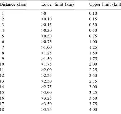
An alternative to a single value of I for the whole sample is given by the spatial correlogram (Cliff and Ord, 1981). This is based on the division of all dis-tances found between pairs of plots in several distance classes, and on the retrieval of a different value of I for each one of these classes. The division is usually made by assigning a connection of 1 to all pairs of plots with a distance value included in the class being anal-ysed and a connection of 0 to all other pairs. Hence, the similitude of values of pairs of plots located within some range of distances apart are quantified. It should be noted that values ofwij and st will vary between
distance classes. Information on spatial correlograms is usually given in a visual way by means of graph-ics. Distance classes used in this study are shown in Table 2.
Additionally, as pointed out in the Section 1, if the effect of other factors on the variable analysed has been previously studied by fitting a linear model (and the model fitted is statistically significant) it may be more appropriate to calculate I using the residuals of the fitted model (also using Eq. (1)).
There are several approaches to test the significance of I against the null hypothesis that there is no
auto-Table 2
Intervals of the distance classes used in the correlograms Distance class Lower limit (km) Upper limit (km)
correlation. The most commonly used approach sup-poses approximate normality of zi (where zi may be the original or the residual centred values). Formulas for the expectations (E[I]) and variances (Var[I]) under the null hypothesis and normality of ziare given in the Appendix A (note that these change when regression residuals are used instead of the original data). Finally, as shown in Cliff and Ord (1981), the values of I un-der the null hypothesis can be expected to be normally distributed for samples bigger than 50, which allowed testing their significance through the comparison of the standardised deviates [I−E(I )]/√[Var(I )]
against those of the standard normal distribution.
3. Results
3.1. Regional variability and physical variables
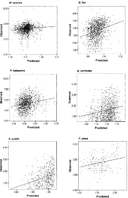
Information from the regression models of the dif-ferent species selected by the stepwise procedure is shown in Table 3 and Fig. 2. In all models the BA was modified (by a logarithmic or square root transforma-tion) to improve the distribution of the residuals. Fur-thermore, these transformations usually lead to better fittings. In some cases a small number of points were rejected as outlyers.
Table 3 and Fig. 2 clearly show that, in general, the fittings achieved in all models were low. No model could explain more than 10% of the variability observed in the BA (given by the determination coef-ficient). From the point of view of the regional vari-ability, these results were not completely unexpected since the study area was relatively small. Conversely,
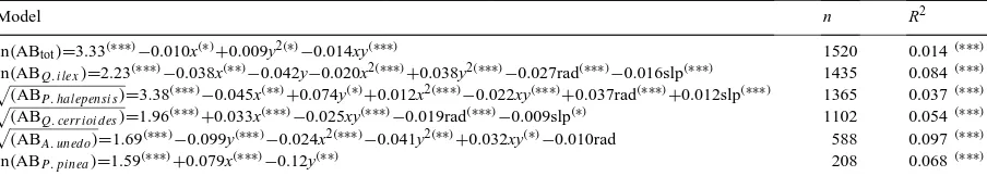
Table 3
Models built by the stepwise procedure applied to join data (ABtot) and to each one of the species separatelya
Model n R2
aIndependent variables selected are multiplied by their respective partial regression coefficients. The statistical significance of the
coefficients, the general statistical significance and the degree of fitting are also given. rad: mean value of the daily potential solar radiation for all year on the plot, slp: slope of the plot, n: number of plots used in the fitting, R2: determination coefficient (%), ln: natural logarithm, √
: square root, *: p<0.05, **: p<0.01 and ***: p<0.001.
a much more clear effect could be foreseen for the slope and the relief. On the other hand, in spite of the low R2 values achieved and as a consequence of the large sample sizes, the effect of many of the independent variables was supported by a clear sta-tistical significance. Hence, these variables had (with high probability) an effect on the BA, although such effects were obviously low in magnitude.
The model that considered the total BA values in plots had the lowest fitting. In this model, xy is by far the most significant variable (displaying a negative sign). Hence, the model pointed to a slightly higher BA in the NW and SE parts of the study area (where
xy always attained negative values). Concerning the
slope and the radiation, there seems to be no general effects (the same total BA is expected regardless of their values).
The Q. ilex model achieved a comparatively much higher fitting. However, the regional pattern of the BA was complex and difficult to understand. Notwith-standing, slope and radiation effects were clear: there seemed to be higher BA values of Q. ilex in areas with lower radiation and lower slope (both variables have negative significant coefficients in the Q. ilex model of Table 3). These areas were the valley bottoms, with deeper soils and less water deficit in summer.
P. halepensis BA had a relatively poor fitting, with
Fig. 2. Plots of observed versus predicted values for the regression models described in Table 3.
The regional variables pointed to highest BA val-ues of Q. cerrioides in the SE part of the park (which agrees with a more spread distribution of this species in that area). On the other hand, similar results to those of Q. ilex were found with reference to the effect of slope and radiation. This may be ascribed to ecologi-cal aspects coming from their phylogenetic closeness, but could be also caused by a previous similar man-agement.
The highest fitting was achieved with the BA of
A. unedo. However, it was not significantly affected
by slope and radiation, and its spatial distribution in the study area was quite complex. From the high sig-nificance of (−) y and (−) x2the largest values of BA were expected in the southern central area.
3.2. Autocorrelation analysis
Since models fitted in the previous section were sta-tistically significant, I was obtained from the residuals of the regressions built. This allowed the minimisa-tion of the effect of regional trends, of the slope and of the radiation over the analyses of autocorrelation. The expected moments of values of I calculated from residuals were used to test for the presence of auto-correlation (see the Appendix A).
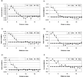
Correlograms from the residuals considering the 18 distance classes given in Table 2 were derived. Since each of the I obtained in every distance class was tested against the null hypothesis of no autocorrelation, a Bonferroni approximation was applied to deal with such simultaneous tests (Rawlings et al., 1998). Thus,
Fig. 3. Correlograms of the residuals of models fitted (see Table 3) considering (a) the total BA of the plot, (b) the BA of Q. ilex, (c) the BA of P. halepensis, (d) the BA of Q. cerrioides, (e) the BA of A. unedo and (f) the BA of P. pinea. Significant values of I are pointed by vertical lines. I obs: observed value of I for a specific distance class, E(I): Expectation of I under the null hypothesis for the specified distance class. The range of distances included in each one of the distance classes is given in Table 2.
to keep a joint significance level (α) of 0.05 for all 18 classes of a correlogram, a more restrictiveα′ of 0.0028 (α′=0.05/18) was applied to each single test.
Correlograms derived are shown in Fig. 3. When values of I are approximately compared to the range of values to be expected from a Pearson correlation co-efficient, it becomes clear that autocorrelations found were low. In general, maximum values achieved were lower than 0.2. However, and in spite of the highly con-servative Bonferroni thresholds, many I values were statistically significant. As in the regression models of the Section 3.1, this was caused by the large samples available for the species studied.
reason-ably explained by processes occurring at a local scale. However, the negative autocorrelations found at further distance classes are much more difficult to explain in a functional sense and are probably caused by limitations of the rather simple linear models pre-viously fitted. Even so, although significant in some cases, these negative autocorrelations had usually extremely low I values.
Limitations of the linear models were probably more evident in the correlogram of P. pinea. This species achieved the highest positive and negative autocorrelations, the later being unusually high. It should be remembered that, due to a lower sample size, only x and y values were used as independent variables in the trend surface analysis of P. pinea. In consequence, it was likely that these higher I values observed were due to a lower fitting capability of the simpler model derived for this species.
4. Discussion
Overall, the woodlands of the study area did not display strong regional gradients, and they were not affected in a clear way by slope or the mean amount of radiation received. Generally, they feature the great-est part of their variability in short distance ranges (significantly shorter than the minimum distance of 100 m considered in this study). Nevertheless, and be-cause of the large sample sizes available, many subtle effects and tendencies were proven statistically. In consequence, the hypothesis stating that environmen-tal factors will lead to the establishment of prominent spatial patterns on the BA in non-disturbed Mediter-ranean woodlands was not supported by the results of the study.
The most striking outcome of the study probably concerns the low effects of radiation. Since radiation is directly linked to water deficit in summer, it would be expected for a Mediterranean woodland to be largely affected by this variable. However, although the ma-jority of the area had not been timbered for at least 50 years, it possibly still retained some effects of previous management. Indeed, due to the usual low productiv-ity of Mediterranean forests (Ibáñez et al., 1999), con-sequences of activities carried out in the past may last for long periods of time. Another probable explana-tion comes from the fact that woodlands in the study
area are more frequently located on slopes facing east or west. Actually, there is a big contrast between the main south facing part of the study area, adjacent to the city of Barcelona, and the other parts. Due to a high recurrence of fires, this south facing portion has hardly any forest and, in consequence, few survey plots were located in this area. Thus, although impor-tant, this big contrast between south and north facing slopes was omitted in the models fitted in this study.
It might be also suggested that the effect of other non-controlled factors, such as the availability of a lim-iting nutrient (Mayor and Rodà, 1994), has overridden the effects of the radiation. However, unless the spa-tial distribution of these non-controlled factors were highly variable in short spatial distances, their signifi-cant effects would have been reflected through strong autocorrelation values (which were not observed). In fact, the poor fittings of models and low values of au-tocorrelations found suggested that the inner dynamics of BA evolution, during the development of each site, was complex leading to high variability that masked the effect of all environmental factors studied.
Concerning methodological aspects, stepwise meth-ods have been widely (and fairly) criticised as not being reliable under many situations (Sen and Srivas-tava, 1990; Christensen, 1996). Nevertheless, inde-pendent variables selected by the stepwise method used in this study agree almost completely with more significant variables found in models preliminarily fitted with all variables at the same time (results not shown). This agreement probably comes from the large sample sizes available (compared to the num-ber of independent variables tried) and ensures the reliability of the models selected.
On the other hand, the detection of spatial auto-correlation is only evidence for the presence of links between values of spatially related points. These links may, however, be due to many direct or indirect causes. In this study, several biotic (e.g. demographic dynamics and dispersion processes), abiotic (other non-controlled factors besides slope and radiation, with high spatial variability) and human driven factors (similar past forest management in near sites) may have been responsible for the, rather humble, levels of autocorrelation observed.
divi-sion of the spatial variability in three levels carried out in this study was, in some degree, theoretical. Specif-ically, the limit between the regional variability and the autocorrelation processes was, somehow, arbitrary. Both items may be caused by a variety of factors which will not be always exclusive. However, it may be ex-pected for the regional variability to display a gradual trend, while autocorrelation processes are expected to occur locally and, more often, with positive values. Again, it may be expected that the large samples avail-able in this study have led to a fairly good discrimi-nation of both variability levels.
When a significant degree of autocorrelation is de-tected for the residuals, the least square estimates of the regression coefficients, although unbiased, loose their efficiency. Under such circumstances, Cliff and Ord (1981) propose the use of more complex proce-dures that include a spatial autoregressive component in the linear models. Thus, instead of the simple co-variance matrix presumed in the ordinary least squares (σ2I, where I is the identity matrix) a more
sophisti-cated approach may be considered by means of gen-eralised least squares. In this case, the autoregressive structure of residuals is given to the model through a matrix V of order n×n (and the covariance matrix is
presumed to beσ2V). However, although being more
adequate under theoretical grounds, these models are based on often unstable iterative fittings that frequently lead to parameter estimates that are less reliable than those given by ordinary least squares (Rawlings et al., 1998). Therefore, and considering the low autocorre-lations achieved, original models fitted were accepted as valid in this study.
The results of this study also have practical conse-quences. The low autocorrelations observed pointed to poor interpolation capabilities for BA values in the study area. This work showed how plots located 100 m apart have BA values nearly as different as those lo-cated much further away. This has some important im-plications on the design of future forest surveys in the study area. Thus, if mapping of a continuous variable (such as BA) has to be carried out by interpolation, a much denser grid will be necessary, although this may be economically unaffordable. In consequence, remote sensing may be proposed as an alternative to sampling in the field. However, further results sup-porting this option in this type of woodlands are still required (Salvador and Pons, 1998b).
5. Conclusions
Spatial variability of BA of woodlands studied oc-curs within really short spatial ranges (of clearly less than 100 m), and neither the radiation nor the slope seem to have an important effect upon this parame-ter. In consequence, such results do not support the hypothesis giving a prominent role to environmental variables as factors leading to the establishment of sig-nificant spatial patterns of the BA on non-disturbed Mediterranean woodlands. Various factors such as a long term effect of forest management, an uneven pres-ence of relief conditions and a complex dynamics of the BA within plots are suggested as possible explana-tions for the results found. On the other hand, the low autocorrelations observed will impose severe restric-tions when interpolating BA values in the study area. This will have practical consequences in the design of forest inventories.
Finally, the following recommendations are sug-gested for future studies concerning spatial patterns in the structure of Mediterranean woodlands: (1) mea-surements at interval distances less than 100 m may be better suited for autocorrelation analyses, (2) the assessment of the effect of different plot sizes may also help understanding the spatial patterns observed. Specifically, block kriging can be applied (Goovaerts, 1997), (3) the usage of a similar methodology in other areas with a more even distribution of geographical conditions (such as a higher proportion of forested south facing slopes) and a wider extension may im-prove the conclusions derived from the present study, (4) new studies should explore the complex effect of interactions between species found in the same plot, and (5) further attempts with high resolution digital imagery may help in the description and understand-ing of spatial patterns in the structure of Mediterranean woodlands.
Acknowledgements
the computer support. Particularly, Xavier Pons of-fered his knowledge and previously developed soft-ware.
The postdoctoral grant provided by the European Commission that I currently hold has allowed me the writing of the manuscript. Finally, I also want to thank David Price and the Editor-in-Chief M.R. Carter for their careful revision of the manuscript.
Appendix A
Formulas for the E(I) and Var(I) under the null hy-pothesis of no autocorrelation, supposing normality of the data. Eqs. (A.1) and (A.2) give the moments to apply when we are working with the original values, and Eqs. (A.3) and (A.4) are the moments to use with residuals of regressions (all of them come from Cliff and Ord (1981) with some slight modifications). As given, Eqs. (A.3) and (A.4) can only be applied when symmetrical connections are used (i.e. wij=wj i for all i and j).
nections, wij the connection between plots i and j,
wi.the sum of all connections involving plot i as the first plot (if connections are symmetricalwi. =w.i),
k the number of independent variables included in the
model+1, X the n×k matrix with the values of all
in-dependent variables given in columns plus an extra column of ones as the first column. W the n×n
ma-trix with allwij values (in Eqs. (A.3) and (A.4) this is expected to be symmetrical), Tr( ) the trace of the matrix, superscript−1 the inverse of the matrix and superscript T is the transpose of the matrix.
References
Burrough, P.A., McDonnell, R.A., 1998. Principles of Geographical Information Systems. Oxford University Press, New York. Canadell, J., Irizar, R., 1988. L’estructura del bosc de la Font
Groga. Patronat Metropolità Parc de Collserola, Barcelona. Christensen, R., 1996. Plane answers to complex questions. In:
The Theory of Linear Models. Springer, New York.
Cliff, A.D., Ord, J.K., 1981. Spatial processes. In: Models and Applications. Pion, Norwich.
Espelta, J.M., Gene, C., Retana, J., Terradas, J., 1992. Structure of mixed holm oak (Quercus ilex) Aleppo pine (Pinus halepensis) forests in Northeastern Spain. In: Teller, A., Mathy, P., Jeffers, J.N.R. (Eds.), Responses of Forest Ecosystems to Environmental Changes. Elsevier, Londres, pp. 892–894.
Goovaerts, P., 1997. Geostatistics for Natural Resources Evaluation. Oxford, New York.
Hellmers, H., Bonner, J.F., Kelleher, J.M., 1955. Soil fertility: a watershed management problem in the Sant Gabriel mountains of Southern California. Soil Sci. 80, 189–197.
Herrera, C.M., Jordano, P., López-Soria, L., Amat, J.A., 1994. Recruitment of a mast-fruiting, bird-dispersed tree: bridging frugivore activity and seedling establishment. Ecol. Monographs 64, 315–344.
Ibáñez, J.J., Lledó, M.J., Sánchez, J.R., Rodà, F., 1999. Stand structure, aboveground biomass and production. In: Rodà, F., Retana, J., Gracia, C.A., Bellot, J. (Eds.), Ecology of Medi-terranean Evergreen Oak Forests. Springer, Berlin, pp. 31–45. Legendre, P., Fortin, M.J., 1989. Spatial pattern and ecological
analysis. Vegetation 80, 107–138.
Mayor, X., Rodà, F., 1994. Effects of irrigation and fertilisation on stem diameter growth in a Mediterranean holm oak forest. For. Ecol. Manage. 68, 119–126.
Montgomery, D.C., Peck, E.A., 1992. Introduction to Linear Regression Analysis. Wiley, New York, pp. 270–274. Oechel, W.C., Lowell, W., Jarrell, W., 1981. Nutrient and
environmental controls on carbon flux in Mediterranean shrubs of California. In: Margaris, N.S., Mooney, H.A. (Eds.), Components of Productivity of Mediterranean-climate Regions. Dr. W. Junk Publishers, The Hage, pp. 53–59.
Pons, X., 1996. Estimación de la radiación solar a partir de modelos digitales de elevaciones. Propuesta metodológica. In: Juaristi, J., Moro, I. (Eds.), Modelos y Sistemas de información en Geograf´ıa. Departamento de Geograf´ıa del Pa´ıs Vasco, Vitoria-Gasteiz, pp. 87–97.
Rawlings, J.O., Pantula, S.G., Dickey, D.A., 1998. Applied Regression Analysis: A Research Tool. Springer, New York. Ripley, B.D., 1981. Spatial Statistics. Wiley, New York. Salvador, R., Pons, X., 1998a. On the reliability of Landsat
TM for estimating forest variables by regression techniques:
a methodological analysis. IEEE Trans. Geosci. Remote Sens. 36, 1888–1897.
Salvador, R., Pons, X., 1998b. On the applicability of Landsat TM images to Mediterranean forest inventories. For. Ecol. Manage. 104, 193–208.
Sen, A., Srivastava, M., 1990. Regression Analysis: Methods and Applications. Springer, New York.