MIXLIGHT: a flexible light transmission model for
mixed-species forest stands
Kenneth J. Stadt
∗, Victor J. Lieffers
1Renewable Resources, Earth Sciences Building 4-42, University of Alberta, Edmonton, Alta., Canada T6G 2E3 Received 1 October 1999; received in revised form 7 February 2000; accepted 11 February 2000
Abstract
We describe the calibration and structure of a multi-species, two-scale light transmission model, and demonstrate its effectiveness for predicting instantaneous light availability at the stand scale across a wide range of forest stand compositions. The model, MIXLIGHT, calculates light transmission through the forest overstory at the stand or microsite scale using standard forest inventory data and two other parameters, foliage area density and foliage inclination. Since MIXLIGHT simulations on both scales are based on a list of individual tree characteristics, it allows for simple manipulation of stand structure to study the effects of silvicultural options on light availability. The two scales allow the input of various kinds of data, allowing predictions from data of different sources and completeness. A simple and rapid method of calibrating the foliage parameters for the species of interest is presented, using measurements of direct-beam light transmission measurements made in the shadows of newly isolated trees. In an independent validation, MIXLIGHT predicted light transmission at the stand level closely for 17 forest inventory plots with a wide range of density and species composition, during leaf-on and leaf-off seasons and under sunny and cloudy conditions. A sensitivity analysis indicated that the influence of the parameters in the model on stand level light transmission predictions was (highest to lowest): foliage area density, crown radius, crown length, and foliage inclination. Nonetheless, a test of the common assumption that the foliage is spherically inclined caused significant underestimation of light transmission. With this flexibility and demonstrated accuracy, we believe MIXLIGHT will provide an accessible and effective tool for forest stand management and regeneration modeling. © 2000 Elsevier Science B.V. All rights reserved.
Keywords: Boreal forest trees; Abies balsamea; Betula papyfera; Populus balsamifera; Populus tremuloides; Picea glauca; Pinus contorta; PAR; Light penetration; Leaf area density; Leaf angle distribution; Spatial scale
1. Introduction
The characterization of light in forests has been a key focus of work on forest community dynamics and
∗Corresponding author. Tel.:+1-403-492-6827;
fax:+1-403-492-1767.
E-mail addresses: [email protected] (K.J. Stadt), [email protected] (V.J. Lieffers)
1Tel.:+1-403-492-2852; fax:+1-403-492-1767.
regeneration. Numerous studies have established the dependence of tree and understory growth on avail-able light in stands (Messier et al., 1989; Lieffers and Stadt, 1994) and microsites (Poulson and Platt, 1989; Alaback and Tappeiner, 1991; Klinka et al., 1992; McLure and Lee, 1993; Poage and Peart, 1993; Run-kle et al., 1995). However, adequate measurement of light is time-consuming due to the heterogeneity in the arrangement and composition of the canopy, diurnal and seasonal changes in solar position and cloudiness,
and leaf-on and off cycles. A number of authors have shown that it is possible to use the well-described laws of solar geometry and information about the canopy structure to predict light regimes in forests at the stand (Norman and Jarvis, 1975) and the microsite level (Grace et al., 1987; Wang and Jarvis, 1990; Pukkala et al., 1993; Canham et al., 1994; Ter-Mikaelian et al., 1997; Cescatti, 1997b; Bartelink, 1998; Brunner, 1998).
Forest tenures often cover large areas of mixed com-position and have various types of inventory data avail-able for management decisions. These inventories may vary considerably, but are frequently based on tree species, diameter and height measurements and may include crown length and width, and stem spatial lo-cation (Vanclay, 1994). There is also a considerable range of stand-tending and harvesting options which have implications for the light regime and vegetation response. However, light models are driven by param-eters that are seldom measured in working forests, and may be poorly structured for simulating the ef-fects of silivicultural treatment. What is required is an easily-calibrated, multi-species model of light avail-ability that is flexible enough to be driven by existing forestry data and produce accurate understory light predictions on a scale appropriate to the data and man-agement goals. Such a model would be of considerable help in studying, planning and managing regeneration in working and research forests (Lieffers et al., 1999). Light availability models developed for forests vary considerably in approach and complexity. The sim-plest fit the Beer–Lambert law empirically, calculat-ing light transmission based on the overlycalculat-ing leaf area index and an extinction coefficient (Monsi and Saeki, 1953; Pierce and Running, 1988). These produce rea-sonable predictions only for a restricted range of solar angles and are limited to stands which are similar to those in which their extinction coefficients were cal-ibrated (Lieffers et al., 1999). Another approach has been to model the forest canopy as a number of hori-zontally homogeneous layers of grouped foliage, each with an appropriate fraction of the canopy leaf area and layer transmission and reflection coefficients. Such a model predicted the light profile well in a pure Sitka spruce plantation (Norman and Jarvis, 1975), but a considerable amount of data was required to generate the model parameters. These models require leaf-area measurements of various complexity, but leaf area is
seldom available in forestry data. They are also lim-ited to stand-level predictions of light only, and do not account for the horizontal spatial variation of light at microsites throughout the stand.
Spatial approaches group foliage into identifiable objects such as individual rows, crowns, crown layers or shoots which are described geometrically as cylin-ders, ellipsoids, quarter ellipsoids or disks with mea-surements to locate these objects in three-dimensional space. Light penetration through these objects is modeled spatially and temporally, given the solar geometry for that latitude and time, and the posi-tion and size parameters of the geometric shapes. Pukkala et al. (1993) tested a crown model of this type in a pure Scots pine stand, Bartelink (1998) and Brunner (1998) tested somewhat similar models in pure Douglas-fir and beech stands, and Canham et al. (1994) and Ter-Mikaelian et al. (1997) developed models for mixed-species stands. These use size- or species-specific estimates of the projected leaf area density within the crown or similar extinction coeffi-cients to compute through-crown light transmission. They do not account for light reflection, but are able to predict the spatial distribution of light at microsites throughout the stand with reasonable accuracy. Lastly, a number of models combine the spatial features of the geometric approach with a homogeneous layer model to deal with light reflection (Grace et al., 1987; Wang and Jarvis, 1990; Cescatti, 1997a). These have shown good spatial accuracy in pure stands, but require a suite of detailed input data.
regressions are used to determine these parameters. A separate table of foliage area density, foliage inclina-tion parameters and the crown shape for each species and/or each crown-class is required. These can be ob-tained following the calibration described here or from other sources. To account for exposure effects, stand slope and aspect are also required. Dates for deciduous leaf-on and leaf-off, and start/end-dates of the grow-ing season can be added to simulate the seasonal light regime. This is critical for accounting for the leaf-off shoulder seasons in the spring and fall which are im-portant for carbon fixation in wintergreen, evergreen and ephemeral species (Hutchison and Matt, 1977; Man and Lieffers, 1997). In large inventoried plots with stem location data available, light modeling can be carried out at the microsite scale. When the stem po-sition data are missing, the inventoried stand is small and dominated by edge effects, or if only a stand-level estimate of light is required, MIXLIGHT will op-erate at the stand scale, using generalized canopy parameters calculated from the tree list. Since canopy parameters can also be obtained from remote-sensing or canopy analysis instruments, the capability to pre-dict stand-level light directly from canopy leaf area index and inclination information is also possible.
In this paper, we present the structure of MIX-LIGHT, describe a simple method of calibrating the foliage area density and inclination coefficients, and validate its stand-level predictions across a wide range of stand types in the boreal mixedwood forest of cen-tral Alberta, Canada. The importance of the key pa-rameters of MIXLIGHT for stand-level estimation are evaluated in a sensitivity analysis.
2. Methods
2.1. Overview
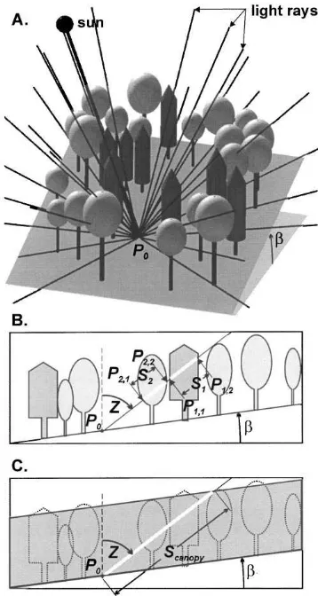
An ideal forest light transmission model would integrate the light-attenuating effect of all foliage po-sitioned between the sky and the measurement point. Since this is seldom possible, a common modeling approach is to sample the intervening foliage by tracing numerous rays from starting points scattered across the sky hemisphere to the measurement point (P0) within the stand (Fig. 1A, Canham et al., 1994; Bartelink, 1998; Brunner, 1998). MIXLIGHT takes
Fig. 1. Overview of MIXLIGHT’s ray tracing approach to light modeling. (A) View of light rays extending from the sun and points scattered across the sky through a stand of trees to the measurement point (P0). For clarity, only 30 rays are shown (a
typical simulation uses 480). (B) Transmission of a ray of light through individual crowns for microsite-level modeling, (C) or through the entire canopy for stand-level modeling. The ray extends from a point in the sky to the measurement point (P0) following
zenith angle Z. Regions (crowns or canopy) that absorb light and contain a random spatial distribution of foliage area are shown in gray. The intersection points between the ray and crowns (Pj1, Pj2)
are shown and the path length through each crown (Sj) or canopy
(Scanopy) is highlighted in white.βis the slope inclination.
or the stand canopy (Fig. 1C). These ray transmis-sion values are weighted by the strength of the light source and averaged to give an estimate of the inte-grated light transmission (the ratio of below to above canopy light) at the measurement point. The individ-ual crown approach (Fig. 1B) accounts for horizontal variation in overstory foliage and produces microsite light predictions, while the canopy scale approach (Fig. 1C) distributes foliage randomly throughout the canopy and produces stand-level predictions. Calibra-tion of the foliage area density and foliage projecCalibra-tion parameters is accomplished by inverting the model-ing process for the simple case of sunlight shinmodel-ing through the crown of an isolated tree (Fig. 2). This is repeated at several times of day at different sun angles, so that the foliage area density and foliage projection parameters can be determined. Simulations are then carried out using these species-specific foliage parameters with the tree lists from the sites of interest.
2.2. Theory
MIXLIGHT models the transmission of photosyn-thetically active radiation (PAR: 400–700 nm). We use ‘light’ as a synonym for PAR, though visible light is a slightly wider waveband. Foliage is taken to include leaves, branches and stem that are contained within the crown or canopy volume since these all attenuate light. Each fragment of foliage area is as-sumed to transmit and reflect no light so that a thin ray of light incident on the forest is either completely absorbed or completely transmitted, depending on whether it hits or misses foliage. If the foliage is ran-domly distributed within the crown or canopy region, the probability that the ray will not be intercepted (P(0)) is given by the Poisson distribution as shown in Eq. (1).
P (0)=T = q[Z, α] q0[Z, α] =
e−
Pn
j=1G[Z,χj]SjFj
(1)
q[Z, α]=q0[Z, α]e−
Pn
j=1G[Z,χj]SjFj
(2)
Eq. (2) is rearranged to yield light flux density (q[Z,α]) rather than transmission (T), which is a more con-venient form for modeling the diffuse and seasonal light flux (see Eq. (4)). In Eqs. (1) and (2), q[Z,α]
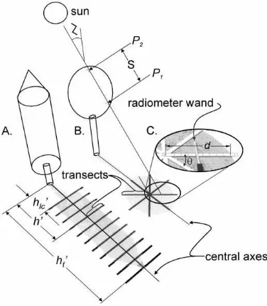
Fig. 2. Calibration of foliage area density and foliage inclination parameters in the shadow of individual trees. (A) Transect layout for rocket (shown), cylindrical, paraboloid and conical crowns. Transects originate at the central axis of the shadow and ex-tend perpendicularly (one in each direction to the shadow edge). Measurements of shadow ‘height’ (h′
t), transect ‘height’ (h′) and
shadow height to live-crown (h′
lc), all with respect to the base of
the stem, are shown. (B) Transect layout for ellipsoidal crowns. Transects originate in the center of the crown shadow and extend to the shadow edge. A ray of sunlight passing through the crown to one of the transects is shown: Z is the solar zenith angle, P1
and P2 are the intersection points of the ray with the crown, and
S is the path length of the ray through the crown. (C) Detail of a single transect showing a light measurement with the radiome-ter wand held at right angles to the transect.θ is the angle made by the transect and the central axis of the shadow and d is the distance from the transect origin to the shadow edge.
the Beer–Lambert law (Swinehart, 1962), we consider the product G[Z,χj]SjFj (=−ln T) as the absorbance for the region j. Since absorbances are additive, the summation in Eqs. (1) and (2) deals with any num-ber of light absorbing regions (n) that intersect the light path, from a single canopy (n=1, Fig. 1C) to an array of individual crowns (n=number of trees, Fig. 1B).
Tdiffuse or seasonal =
Qdiffuse or seasonal
For instantaneous estimates of light transmission, Eq. (2) is applied once for direct-beam radiation transmis-sion (Tdirect) using the sun’s position angles (Zs,αs; Eq. (3)), and multiple times using angles identify-ing the centers of equal-area sectors of the sky (i.e. sky-elements of equal solid angle) for integrating the transmission of diffuse or seasonal skylight (Eq. (4)). (Note that Eq. (3) simplifies to Eq. (1) since only one ray is traced). In Eq. (4), c=1,. . ., nc is the in-dex for the zenith angles (Zc) which are divided into
nc equal increments of the cosine of the zenith from
1 (Zc=0◦) to 0 (Zc=90◦) to achieve equal-area sam-pling of the sky, and a=1,. . ., na is the index for the azimuth angles (αa) which are divided into na equal increments from 0 to 360◦. The flux densities of all rays are cosine-corrected to the flux density through a horizontal surface. For daily or seasonal transmission, we followed the example of Canham et al. (1994) and generated a ‘seasonal sky matrix,’ which adds to the diffuse skylight the flux density of the sun while it passes through each sky sector and is not obscured by cloud. Eq. (4) is then applied, using the Z,α coordi-nates of each of these sectors and the incident seasonal light flux density (q0[Z,α]) calculated for the sector. With this approach, light availability can be calculated seasonally or for specific times of the year and day, and for various weather conditions.
2.3. Study area
Calibration and validation of MIXLIGHT were performed in a number of stands across west-central Alberta (53◦30′–54◦10′N, 114◦50′–118◦W). Mean annual temperature in this region is 0.9–2.6◦C, and precipitation is 530–560 mm per annum, approxi-mately 60% of it falling during the growing season (May–August) (Anonymous, 1982a, b). All stands were upland sites with submesotrophic to mesotrophic nutrient status and mesic to hygric ecological mois-ture regime (Anonymous, 1994)
2.4. Model calibration
2.4.1. Foliage area density
The foliage area density of various tree species was determined on newly-isolated residual trees on clearcut edges and in partial-cut stands. We visited 10 cutblocks from late June to August in 1996 and 1997 for leaf-on calibration, and in April 1997 for leaf-off measurements. Before cutting, the sites were domi-nated by either aspen (Populus tremuloides Michx.), white spruce (Picea glauca (Moench) Voss) or mix-tures of these, balsam fir (Abies balsamea (L.) Mill.), balsam poplar (Populus balsamifera L.), and white birch (Betula papyrifera Marsh.). Trees were mea-sured as soon as possible after logging (1 week–3 months) so they still retained most of the leaf and shape characteristics they had while growing in the stand.
Light measurements were taken with an 80 sen-sor linear radiometer (Model SF-80, Decagon De-vices, Pullman, WA) which measures PAR in quan-tum units (mmol m−2s−1). Measurements were made during periods of direct sun when the trees cast a clearly delineated shadow on the ground. At each sample tree, crown width, total shadow length (h′t, stem base to shadow apex), length to the base of the shadow’s live-crown (h′
were used to sample ellipsoidal crowns (Fig. 2B). To compensate for the horizontal movement of the sun (0.25◦min−1), the origin of each transect was aligned with the central axis of the shadow before commenc-ing each transect. Vertical changes in the sun’s position (<0.1◦min−1) were small enough to be ignored during the sampling period. Where necessary, ground slope and aspect were measured to later transform the tran-sect positions to horizontal coordinates. Every 50 cm from the transect origin, the radiometer wand has held at right angles to the transect (Fig. 2C), six light mea-surements taken over 6 s and the average recorded. Sampling extended 100–150 cm past the edge of the shadow to provide at least one unshaded light measure (Q0) for that transect. Length from the transect ori-gin to the shadow edge (d, Fig. 2C) was recorded for crown size determination. Total (Q0) and diffuse light (Qdiffuse) were measured in unshaded sunlight adja-cent to the crown shadow immediately before and af-ter sampling each tree by exposing then shading a sin-gle sensor of the radiometer with a small disk at 2 m distance, and recording the output from that sensor. Sampling time depended on tree size, but was usually less than 20 min per tree.
An appropriate geometric shape (ellipsoid, paraboloid, cone, cylinder, or rocket (a cone of 25% of the crown length perched on a cylinder 75% of the crown length)) was chosen for the crown of each species (Table 1). To obtain the dimensions of these shapes (crown length (tree height minus live-crown height) and radius), actual height and live-crown height measurements were adjusted for the solar zenith angle at the time of measurement (Eq. (5)).
actual length= shadow length tanZs
(5)
We assumed the crowns were circular in cross-section so that their crown radius was not affected by solar angle. The solar zenith and azimuth at the time, day, latitude and longitude of measurement were obtained using the formulae of Iqbal (1983).
The transmission of direct beam light (Tdirect) was calculated by subtracting the diffuse component (Qdiffuse) from the light measured (Q) at the point and from the light measured outside the crown shadow (Q0), then taking the ratio of these two (Eq. (6)).
Tdirect=
Q−Qdiffuse
Q0−Qdiffuse
(6)
The diffuse light actually decreases for measurements nearer the tree since its stem and crown capture more of the diffuse light. The effect on direct-beam trans-mission and the resulting increase in the foliage den-sity estimate that results from this is small, however, because the direct-beam flux is so much greater (>4 times) than the diffuse. The path length of the sun through the crown (S, Fig. 2B) was estimated by solv-ing for the intersection of the ray vector described by the measurement point and the sun angle with the ge-ometric crown. Equations for determining the two in-tersection points (P1(x1, y1, z1) and P2(x2, y2, z2)) for a ray passing through the various crown shapes are presented in Appendix A. The distance formula (Eq. (7)) was then applied to the intersection points to ob-tain the path length.
S=
q
(x2−x1)2+(y2−y1)2+(z2−z1)2 (7) The projection of a unit of foliage area in the sun’s direction (G[Zs,χj]) was calculated using Eq. (9), as described below. Lastly, the foliage area density (Fj) was calculated from these variables by inverting Eq. (1) (see Eq. (8)).
Fj = −
lnTdirect
G[Zs, χj]S
(8)
Foliage densities were averaged over all measurement points within each tree’s shadow. Trees were then av-eraged within a species to yield that species’ average foliage area density. Estimates calculated from radial transects were weighted by the length from the tran-sect origin to the measurement point to even out the area sampling rate.
2.4.2. Foliage inclination and projection
parameter, the ratio of vertical to horizontal projec-tions,χj. Whenχj=1, the foliage inclines as if cov-ering a sphere: smaller values indicate mostly vertical foliage area orientation, largerχjindicate mostly hor-izontal foliage. The projection of an ellipsoid, having a surface area of 1, perpendicular to the light source zenith is given by Eq. (9) (Campbell and Norman, 1989).
G[Z, χj]=
q
χj2cos2Z+sin2Z
χj+1.774(χj+1.182)−0.733
(9)
Campbell and Norman (1989) also demonstrated how the inclination (χj) parameter can be obtained by measuring the gap fraction at a number of zenith angles (Z), then solving for foliage area and foliage inclination using inversion techniques. We used direct sunlight transmission as a measure of gap fraction in individual crowns then corrected for any change in the path length (S) with solar zenith angle (Zs) to yield the dependent variable−ln(Tdirect)/S. We found the incli-nation and foliage area density (Fj) parameters that offered the best fit to Eq. (10) by nonlinear regression of−ln(Tdirect)/S on the independent variable Zs. −lnTSdirect =G[Zs, χj]Fj (10) A similar approach suing sunlight transmission ap-proach to obtaining G for particular solar angles when F is known is demonstrated by Oker-Blom et al. (1991).
Direct-beam light transmission data taken at a num-ber of solar angles were obtained from a study by Constabel (1995). She sampled 10 aspen, 10 overstory white spruce and 10 understory white spruce trees on 22 June 1994 in a partially-cut mixed forest in central Alberta (53◦40′N, 116◦40′W). Each crown was suffi-ciently isolated that it cast a distinct shadow through most of the day. Shadows were sampled during five 1 h periods with mean solar zenith angles of 30.7, 32.9, 35.7, 51.2 and 65.3◦. At each sampling time, nine light measurements (Q) were taken in the crown shadow of each tree, with the 80 cm radiometer wand held par-allel to the stem. Three measurements were taken at random positions in the upper third of the crown, three in the middle, and three in the lower third, then aver-aged for each tree. Total (Q0) and diffuse flux density (Qdiffuse) were measured in full sun adjacent to the
crown shadow immediately before and after sampling each tree as outlined for the foliage area density mea-surements above. Tree height, ht, live-crown height,
hlc, and crown width, cw, were determined with a cli-nometer and measuring tape.
With this data, we calculated direct sunlight trans-mission through the whole crown by subtracting the diffuse component as above (Eq. (6)). Since the mea-surement points were not mapped spatially (to speed sampling), we had to simplify the crown shape. We first determined the volume of each crown as either an ellipsoid (aspen) or a rocket (white spruce) using the crown length and width to establish the axis lengths. We then redefined the crowns as rectangular solids with one side facing the sun, one crown length deep and of equal length and width such that they contained the same volume as the original shape.
S= w
sinZs
(11)
The path length of light through the crown (S) at the solar zenith (Zs) was calculated using the width (w) of the rectangle (Eq. (11)). The negative logarithm of direct sunlight transmission was then divided by S, to yield the dependent variable in Eq. (10). We used the derivative-free nonlinear regression method available in SAS release 6.12 (PROC NLIN METHOD=DUD, SAS Institute, Cary, NC) to regress−ln(Tdirect)/S on
Zs (Eq. (10)) and obtain χj and Fj. These parame-ters were calculated for each tree, then averaged for the species. Since the measurement points were not well-mapped, only the inclination parameter (χj) was used.
2.5. The MIXLIGHT model
2.5.1. Crown-scale modeling
At each measurement point, diffuse skylight trans-mission was calculated by averaging the transmis-sion along at least 480 light paths (Eq. (4): na=24 equally spaced azimuths from 0 to 360◦, and nc=20 zeniths, spaced by equal increments of the cosine of the zenith from 1 (0◦) to 0 (90◦)). Each path was checked for slope, stem and crown hits. If the light source was obscured by the sloping ground (Eq. (12)), a value of 0% light transmission was returned for that path.
cos(1s)=cosβcosZ+sinβcos(α−) (12)
Here, cos(1s) is the cosine of the angle between a
line perpendicular to the slope and the light source,
β is the slope inclination, andthe slope aspect. If cos(1s)<0, the source is obscured by the slope. Stem hits were determined by checking the paraboloid stems for an intersection with the light path using the simul-taneous solution to the ray and paraboloid equation (Appendix A). Any stem hit caused 0% transmission to be returned for that path.
In the absence of these, ray transmission was de-termined by the length the light ray passed through each crown of the various trees between the sim-ulation point and the sky. Again, the simultaneous solution to the ray and geometric crown equation (Appendix A) was used to determine intersection points, and Eq. (7) applied to obtain the length of the ray between these points (S). This ray length was multiplied by the foliage projection and foliage area density for the appropriate species to give an absorbance (Aj=G[Z,χj]SjFj), which was summed for all crowns encountered on the path. The sum of these absorbance values along each light path was then converted back to a flux density (q[Z,α]), as shown in Eq. (2). We used the uniform overcast sky (UOC) assumption for diffuse light, i.e. light incident from all equal-area sectors of the sky was assumed to have equal flux density.
Direct sunlight absorbance was obtained in a sim-ilar way, but for only one light path using the solar zenith and azimuth angle at the date, time and loca-tion of measurement. The proporloca-tions of direct and diffuse light at the time of measurement were applied to the output to give the integrated light transmission prediction.
2.5.2. Canopy-scale modeling
To avoid excessive edge effects, crown scale modeling requires a large area of inventoried trees surrounding a much smaller central area in which pre-dictions are made. This allows ray-tracing to proceed to wide zenith angles without encountering the plot edge. For example, in a 50 m×50 m flat inventory plot with 20 m tall trees and with the measurement point at plot center, 51◦ is the widest possible zenith angle that will still avoid the plot edge. Although the light ray transmission values are weighted by the cosine of their zenith angle, nearly 40% of the weight of the diffuse light measurement would be obtained from zenith angles larger than 51◦since there is so much sky area beneath this angle. Light transmission is low at large zenith angles owing to the long path through the canopy, so ignoring these angles would inflate the transmission estimate.
A stand-level light modeling scale can be used when edge effects are large or when the input data lack a stem map. This scale assumes the foliage is carried randomly within the space above the entire stand. Leaf area index (LAI) measuring devices such as the plant canopy analyzer (LAI-2000, LI-COR, Lincoln, NB) use this model scale to calculate LAI and the mean inclination angle of the leaves from measurements of transmitted diffuse light. MIXLIGHT provides a pro-vision to input plant canopy analyzer measurements directly.
However, since LAI measurements are seldom obtained in forest inventories, MIXLIGHT can also estimate the leaf area contained within the trees in the inventory list. Our measurements of foliage area den-sity (F, see Section 3) did not suggest a change in Fj with tree size: trees of the same species maintained a similar foliage area density regardless of their crown volume. We therefore calculated stand-level foliage area density (Fcanopy) as the sum of the foliage area contained in each tree crown (the product of crown volume, Vj, and crown foliage density, Fj) plus one half the surface area of each stem (Bj), divided by the canopy volume (Vcanopy=plot length×plot width×average canopy tree height×cosβ, whereβis the slope inclination) (Eq. (13)).
Fcanopy=
Pn
j=1(VjFj +(1/2)Bi)
Vcanopy
Half the stem surface area is used since the light rays can only hit one side of the stem at a time. The volume of the geometric crowns and the surface area of the paraboloid stems (Bj) were calculated using standard equations (Glover, 1996).
The projection of the foliage for stand-level model-ing was treated differently than for individual crowns. In order to incorporate the effect of the below-crown stems (which we treated as truncated paraboloids) the projection of a unit of canopy foliage (Gcanopy[Z]) was determined separately for every zenith angle used in ray tracing (the angles used in Eqs. (3) and (4)). Again, the foliage projection was assumed constant with respect to the azimuth.
Gcanopy[Z]=
Pn
j=1(VjFjG[Z, χj]+(4/3)rjhjsinZ)
Fcanopy
(14)
The projection fraction for each zenith angle (Gcanopy[Z], Eq. (14)), is the sum of the projected area of the crown foliage at this angle (crown volume×crown foliage area density×crown foliage projection) plus the projected area at the same angle of the below-crown stem of each tree, divided by the total one-sided foliage and stem surface area (Fcanopy, Eq. (13)). For simplicity, we treated the stem projec-tion as the projecprojec-tion of a parabola with one face to the light source, which underestimates the projected area significantly only for very small zenith angles. In Eq. (14), rj is the radius at the base of the paraboloid stem and hj is the tree height.
Light transmission is calculated as for the crown-scale model, except that there is only one ob-ject (n=1 in Eq. (2)) and the path length through the canopy is simpler to determine.
If the canopy is the height of an average canopy tree (hcanopy) and extends ‘horizontally’ (or following a constant ground slope) to infinity, the path length of a ray through the canopy (Scanopy, Fig. 1C) is given by Eq. (15), where z0 is the height of the measure-ment point, Z andαare the zenith and azimuth of the light ray, φ is the apparent slope in theα direction, and β and are the slope inclination and aspect, respectively.
Scanopy=
(hcanopy−z0)cosφ cos(Z−φ) ,
φ=arctan [tanβcos(α−)] (15)
2.6. Stand level validation
Alberta Forest Service permanent sample plots (PSPs) were used to apply and test the instantaneous predictions of MIXLIGHT on a stand level. We se-lected 17 upland PSPs, with species compositions ranging from dominance by pure aspen, white spruce, or lodgepole pine, to mixtures of these and balsam poplar, white birch and balsam fir. These PSPs were square plots, 900–1600 m2 in area, with stem densi-ties of 335–1420 stems ha−1, and stand age (all sites were fire-initiated) from 69 to 159 years. We sampled 16 plots during the deciduous leaf-on period (mid June–early September) in 1996 and 1997, and remea-sured eight, plus one new one, in the leaf-off period (April 1997). Light measurements were made with the same linear radiometer as the calibration measure-ments, either during mostly cloudy (no direct sunlight) or mostly clear (>80% of light from the sun) periods. Light was sampled above shrub height (∼1.5 m) for 36–49 points following a 5 m×5 m grid pattern. At each point, 12 light readings were taken at 30◦ incre-ments while sweeping the radiometer wand around a horizontal circle at arm’s length: the mean of these 12 flux density measurements was recorded. These values were expressed as a percentage of the above-canopy light averaged for 5 min before and 5 min after the within canopy value was taken. Above-canopy light was measured by a point quantum sensor (LI-190SA, Li-COR, Lincoln, NB) and datalogger (CR21X, Campbell Scientific, Logan, UT) in a nearby clearing. These 36–49 transmission measurements were then averaged to give the stand-level light transmission value.
and estimated height, height-to-live-crown, and crown radius for each tree. The tree lists were loaded into the model along with the appropriate site information (latitude, longitude, slope, aspect, plot dimensions, date and time of measurement, percentage of diffuse light at time of measurement) and the species-specific parameters (crown shape, crown foliage area density and crown foliage inclination). Canopy-scale model predictions were then compared to the measured values of light transmission on a stand-average basis.
2.7. Model sensitivity and foliage inclination
The model was evaluated for the sensitivity of its light transmission predictions to the inputs on a stand level. This sensitivity analysis was performed using tree lists from three stand types: deciduous-dominated, mixed conifer-deciduous with some large (80 m2) gaps, and a conifer stand. For each sensitivity run, we altered one of four key parameters across all species. These parameters were the species-specific foliage area density (F) and ellipsoidal leaf inclination param-eter (χj), the crown radius (cr), and the crown length (cl). Note that this was a test of the sensitivity of MIXLIGHT’s stand-level predictions, so varying the crown size parameters altered the model predictions through their effect on the calculated canopy foliage area and projection. They were included nonetheless, since the model is driven by these individual tree measurements. The other parameters not tested are measured with a much higher degree of accuracy (lat-itude, long(lat-itude, slope, aspect, plot dimensions, date and time of measurement, percentage of diffuse light at time of measurement, tree coordinates). The tested parameters were varied one at a time through a set of logarithmic multiples over seven runs: 2−2, 2−1, 2−0.5, 20, 20.5, 21, and 22 (25, 50, 71, 100, 141, 200, and 400% of the original value). Instantaneous light trans-mission predictions on cloudy (100% diffuse light) and sunny (90% direct sunlight) days were compared. Since other models have not attempted to account for the effects of foliage inclination (Grace et al., 1987; Pukkala et al., 1993; Canham et al., 1994; Brunner, 1998), and some effort is required to cali-brate this parameter, we also tested MIXLIGHT on the validation sites with the foliage inclination pa-rameter set to spherical (χj=1) for all species. This required small corrections to the foliage area density
estimates, since they were adjusted for projection during calibration (Eq. (8)).
3. Results
3.1. Calibration
Calibration trees were sampled in 10 harvested ar-eas. Generally, each species was sampled in at least at two different sites, except for lodgepole pine for which only one suitable partial-cut site was available. Tree size spanned the range of sizes which might be ex-pected in mature stands (Table 1). Selection of the ap-propriate geometric crown shape was straightforward. Early self-pruning and die-back of the lower branches made an ellipsoid shape appropriate for the deciduous and pine crowns. Continuous branch growth with the development of a slight sag made a paraboloid fit the fir crowns well, and the rocket (cone over cylinder) shape was superior for white spruce because of the increasingly pronounced branch sag from the mid to lower crown.
Individual fir crowns transmitted the least light, fol-lowed by overstory white spruce, understory spruce, pine, and leaf-on birch, aspen, and balsam poplar (Ta-ble 1). During the leaf-off season, light transmission through deciduous crowns was roughly doubled. In 50 of the 57 trees sampled, and without apparent bias as to species or size, the light absorption value calculated at each measurement point within the crown shadow was significantly correlated with the calculated path length of the sun ray through the geometric crown to that point (P<0.05), indicating that path length can account for at least some of the variation in transmit-ted light. Regression analysis indicatransmit-ted that the effect of path length on light absorbance (−ln T) was linear, so Eq. (8) should provide appropriate estimates of foliage area density.
within each species (data not shown); this param-eter appears to be constant within the size range of trees measured. Foliage inclination, measured in leaf-on aspen and white spruce only, tended from mostly vertical for overstory spruce (χj=0.10 as much straight-down as sideways projection) to half as much horizontal projection as vertical (0.53) for un-derstory spruce, to close to spherical (0.82) for aspen (Table 1).
3.2. Validation
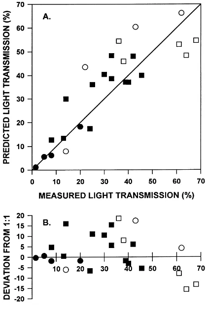
MIXLIGHT predictions of instantaneous stand-level light transmission were well-correlated with mea-sured light transmission (Fig. 3, Pearson’s r=0.86,
n=25, P<0.0001). The slope of the predicted ver-sus measured relationship (1.03) for a regression constrained to pass through the origin was not signifi-cantly different from the ideal slope of 1 (P=0.5606). For some medium-light sites, MIXLIGHT predicted higher light levels than were actually measured by as much as 22% absolute transmission (44% transmis-sion predicted for a site with 22% measured light). There was also a tendency to underestimate transmis-sion to high-light sites (which were measured under leaf-off conditions): the worst was 48% transmission predicted for a site in which 64% was measured. The residual plot suggests a curvilinear relationship (Fig. 2B). Indeed, a quadratic equation with inter-cept had a better fit (adjusted R2=0.81) than the linear, zero-intercept equation (adjusted R2=0.69). Analysis of the residuals from a 1:1 relationship also showed that the deviations were negatively correlated with increasing site moisture class: overstory light transmission tended to be overestimated in wetter sites and underestimated in drier sites (P=0.0065). No effect of site nutrient status was detectable (P=0.6194).
3.3. Model sensitivity and foliage inclination
Results of the sensitivity analysis of MIXLIGHT at the canopy level were similar under sunny and cloudy conditions. Only the overcast day results, which had slightly more variation, are shown (Fig. 4). Predic-tions were most responsive to foliage area density and crown radius. Doubling or halving the species’ foliage
Fig. 3. MIXLIGHT stand-level validation for 17 sites measured and modeled under various weather conditions and seasons: (s)
leaf-off on a sunny-day, (h) leaf-off on a cloudy day, (d) leaf-on on a sunny day, (j) leaf-on on a cloudy day. Since some sites were measured under several conditions (sun/cloud, leaf-on/leaf-off) there are 25 data points. (A) Predicted instantaneous light trans-mission (% of above-canopy light) is compared to measured light transmission averaged across the stand. (B) Residuals from a 1:1 relationship between predicted and measured light transmission.
incli-Fig. 4. Sensitivity analysis of the (m) foliage area density, (r)
foliage inclination, (d) crown radius and (j) crown length
pa-rameters of MIXLIGHT for three stands: (A) aspen dominated, (B) white spruce/aspen mixedwood with gaps, (C) white spruce dominated. Parameters were multiplied by the percentage shown. Light transmission predictions are instantaneous stand-level pre-dictions for a cloudy day during the leaf-on season.
nation parameter caused the least effect: even extreme (0.25–4 times) variations (e.g. χj=0.026–0.42 for canopy spruce, andχj=0.20–3.3 for aspen) caused a change in the predicted transmission of only a relative 20% from the original transmission value.
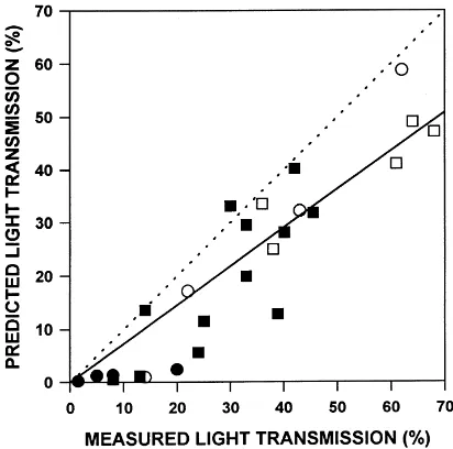
The results of assuming the foliage inclination was spherical for all species are shown in Fig. 5. Light in all sites was underestimated, but the relative error was particularly high for the low-light sites. Model pre-dictions are still precise and capture slightly more of the site-to-site variation (adjusted R2=0.82 when the spherical assumption was used, versus 0.69 with the measured foliage inclination parameters), but consis-tently predict lower values.
Fig. 5. MIXLIGHT stand-level validation with the foliage inclina-tion parameter (χj) set to 1 for all species. Same 17 sites as Fig.
3, measured and modeled under various weather conditions and seasons: (s) leaf-off on a sunny-day, (h) leaf-off on a cloudy
day, (d) leaf-on on a sunny day, (j) leaf-on on a cloudy day.
Pre-dicted instantaneous light transmission (% of above-canopy light) is compared to measured light transmission averaged across the stand. The dotted line is the 1:1 relationship.
4. Discussion
Models for predicting forest light regimes are well-developed, ranging from relatively simple stand models to complex microsite models which rely on detailed measurements of individual-crown or shoot architecture (Cescatti, 1997a, b; Brunner, 1998). To our knowledge, none of these models have been extensively tested in numerous forest stands, a neces-sary prerequisite for applying a light model to track forest regeneration and stand development. This is likely due to model inflexibility or the quantity and complexity of the data required to drive these models. MIXLIGHT, on the other hand, is designed to apply existing theory to the data presently available to a forest manager, and make understory light predictions at a scale appropriate to the data and the goals of the manager.
sunny and cloudy conditions (Fig. 3A). Validation stands varied from highly structured mixtures of tree species in patches with gaps to closed, single-species, single-strata canopies. It appears that MIXLIGHT can capture much of the site-to-site variation in light transmission based on inventory data and the two species-specific foliage parameters. It should thus be an effective modeling tool for managing understory regeneration and vegetation in extensive forest areas.
For canopy-scale modeling, MIXLIGHT requires only a list of the trees, with species, stem diameter, height and crown dimensions (length and width), which are often available in standard forest inventory data, plus species-specific foliage area and inclina-tion parameters. Stem diameter to height funcinclina-tions are available for tree species in many forest districts; we were also able to develop reasonable diameter to live-crown height relationships if stand characteristics are included. A predictive function for crown width or radius has proved more elusive. This parameter is affected by crown abrasion from snow and wind (Grier, 1988), as well as by stand density and compo-sition. Good within-stand relationships were obtained using only stem diameter and species as predictive variables, but we are currently collecting more exten-sive data on crown width in hopes of developing a site-independent equation. In principle, these relation-ships could reduce MIXLIGHT data requirements to the two foliage parameters, site attributes (plot loca-tion and size, slope, and aspect) and a list of species with their stem diameter.
Leaf area is the most critical driving variable in light transmission modeling (Sampson and Smith, 1993), but is also a difficult parameter to measure. Allomet-ric equations are commonly used to relate leaf area to stem diameter or sapwood area (Pierce and Running, 1988; Oker-Blom et al., 1991; Pukkala et al., 1993) but require considerable effort to calibrate. Branch and stem area must be also be estimated, as these also ex-tinguish light. Light interception techniques (Welles and Cohen, 1996) provide a simpler method to es-timate shading leaf, branch and stem area. Gener-ally these techniques are applied to entire canopies, but Lang and McMurtrie (1992), Acock et al. (1994) and Villalobos et al. (1995) have demonstrated how these methods can be applied to individual plants. For small plants, particularly where the foliage distribu-tion is non-random, this method may underestimate
foliage area (Lang and McMurtrie, 1992). Villalobos et al. (1995), however, found reasonable estimates of single-tree foliage area using light interception meth-ods with larger olive trees. Our calibration trees had large (>2 m long) crowns and all species demonstrated a linear relationship between the negative logarithm of direct-beam light transmission and path length, which suggests a random foliage distribution. We did not in-dependently verify our foliage density estimates, but our data do meet the theoretical requirements for ef-fective estimation by the light interception technique. Our leaf-on foliage area estimates are slightly higher than values reported for similar species. One-sided lodgepole pine needle area density, calcu-lated from the data of Oker-Blom et al. (1991), was 0.4–1.8 m2m−3, which includes a lower limit than we found in our data for trees of similar crown volume. Engelmann spruce (Picea engelmannii Parry ex En-gelm.), in the same study, had a needle area density of 0.6–1.9 m2m−3, while our white spruce (which are similar in profile), had a foliage area density of 0.8–2.6 m2m−3. Our estimates include within-crown branch and stem area, which largely accounts for the differences (Oker-Blom et al. (1991) assumed the branch area was 15% of the needle area). An interesting contrast is with the New England for-est species studied by Canham et al. (1994). They report ‘absolute path length extinction coefficients’ which are mathematically equivalent to projected fo-liage area density. This parameter can be obtained from our calibration data by dividing the negative logarithm of direct-beam light transmission by path length and assuming the projection (G) remains a constant for all light source angles (a spherical dis-tribution of foliage inclination angles). The range of projected leaf area density was 0.07 m2m−3 for red oak (Quercus rubra L.) to 0.32 m2m−3for white pine (Pinus strobus L.) while the range for our bo-real species was 0.20 m2m−3 for balsam poplar to 0.99 m2m−3 for balsam fir. Boreal trees appear to have more compact, denser crowns.
where the relative error would be greater and where the light compensation points of boreal tree and un-derstory species occur (e.g. Greenway, 1994; Man and Lieffers, 1997). The sensitivity analysis indicated that the prediction range corresponding to the abso-lute variation found in the foliage area density (0.5–2 times the average value, Table 1) was similar in mag-nitude to the largest prediction error for the validation (Fig. 4). No trends were found between foliage area density and tree size or site nutrient status; however, deviations from the measured values were correlated with site moisture index. Since leaf area for aspen in particular appears to be limited by moisture (Waring and Schlesinger, 1985; Messier et al., 1998), it is not surprising that wetter sites transmit less light than was predicted using the foliage area density of an ‘average’ tree. Fine-tuning improvements to MIXLIGHT could be made by further calibration of the species’ fo-liage area densities for sites of different moisture index.
Light scattering may provide another source of error in the estimation of foliage area and subsequent sim-ulation of light transmission. We assumed that the fo-liage elements transmit and reflect no light, but clearly this is not the case. For simulating light penetration through crowns or a canopy, neglecting light scatter-ing should result in underestimation of the actual light transmission. In calibration, scattering would cause an underestimate of foliage area density. These effects may cancel each other; however, scattering depends on the species mix, leaf age, and leaf area as well as the solar angle (Norman and Jarvis, 1975; Hutchison and Matt, 1976), so its effects are complex. Hutchison and Matt (1976) suggested the contribution of beam en-richment (foliage-scattered sunlight), should be high-est at high solar elevations in fully-leafed canopies (i.e. at midsummer), and lowest in winter, but there is little evidence of such a trend in our data (Fig. 3). Light scattering appears to be a relatively small com-ponent of the understory radiation in our high latitude forests.
Although canopy-scale modeling is more rapid and does not require a stem map, the assumption of random foliage distribution throughout the canopy volume is one which may not be met. The most obvious level of foliage grouping is into crowns. In quite open stands, as might occur following partial-cutting, more light would penetrate the canopy than would be predicted by
a model that spreads the foliage randomly throughout the site. The concave-downward trend in our validation data (Fig. 3) may be caused by foliage grouping in the high-light (i.e. open) stands. Crown-scale modeling may be more appropriate for these situations.
The sensitivity analysis illustrates the behavior of MIXLIGHT under systematic changes to its key pa-rameters. It is clear that foliage area density and crown radius should be estimated with the most care. Crown length and foliage inclination are less critical, partic-ularly if only a relative site-to-site comparison is re-quired. If accurate predictions are required, however, it is clear that even foliage inclination should be mea-sured, since setting the foliage inclination to spherical for the validation sites created a downward bias in the predictions (Fig. 5).
MIXLIGHT provides a flexible predictive light transmission model which predicts instantaneous stand-level light well for a wide range of stand condi-tions. Calibration of species’ foliage area density and inclination parameters can be quickly accomplished by direct sunlight transmission measurements on iso-lated trees. Since so many forest processes are driven by light, we believe MIXLIGHT will provide a use-ful tool for evaluating stand tending and regeneration options in forests of diverse structure with limited inventory data. Work is currently under way to eval-uate the microsite-level predictions of MIXLIGHT on instantaneous and long-term bases. Copies of VisualBasic code for MIXLIGHT are available from the authors.
Acknowledgements
Appendix A
A.1. Light ray equation
The equation of a line containing the light mea-surement point P0=(x0, y0, z0), with vertical (zenith) angle, Z, and orientation with respect to north (azimuth),α, is given by Eq. (A.1)
x =x0+a t, y=y0+b t, z=z0+c t (A.1) where a=sinα, b=cosα, c=cot Z, and t is any real number. The y-axis increases in a northward direction, the x-axis westerly, and the z-axis upward.
A.2. Crown and stem shape equations and intersections with light rays
Conical, paraboloid, cylindrical and rocket shaped crowns are truncated at the base of the live-crown (tree base elevation plus the live-crown height (zb+hlc)) and the at the top of the tree (base eleva-tion plus tree height (zb+ht), the apex of the cone or paraboloid). Crown centers (with respect to the crown length and width coordinates, not the center of mass) are at the point (u, v, w) where u andv are the x- and y-coordinates of the tree base (xb, yb), and
w=zb+hlc+(1/2) cl, cl=ht−hlc. Stems are truncated at the tree base elevation (zb) at the bottom and the live crown height (zb+hlc) at the top. To simplify calibration of the foliage area density and inclination parameters for each tree, the origin (0, 0, 0) was set to the center of the crown shadow (i.e. midway along the crown shadow length and midway across the crown shadow width). For predicting light in a stand, the origin was set to the center of the stand.
Functions describing the intersection between the light ray and each of the geometric shapes were gen-erated by substituting the three elements of Eq. (A.1) into each of the shape equations (i.e. substitute x0+at for x, y0+bt for y, etc.), then solving for t. Since these were lengthy equations, we used mathematical soft-ware (Maple V Release 3, Brooks/Cole Publishing, Pacific Grove, CA) to obtain analytical solutions. Be-low, t is expressed as a function of x0, y0, z0, u, v,
w, cr, cl, hlc and ht. There are always two solutions for t, corresponding to the two intersection points. If
t is a complex number (i.e. m is negative), the light
ray does not intersect the shape. Substituting t back into the light ray equation (Eq. (A.1)) yields the x, y,
z coordinates of each intersection point.
Cylinders were described by Eq. (A.2) and their intersection with the light ray by Eq. (A.3).
(x−u)2+(y−v)2=cr2 (A.2)
t=−x0a+au−y0b+bv±
√m
a2
+b2 ,
m=2x0ay0b−2x0abv−2auy0b+2aubv−a2y02 +2a2y0v−a2v2+a2cr2−b2x02+2b2x0u
−b2u2+b2cr2 (A.3)
Cones were described by Eq. (A.4) and their intersec-tion with the light ray by Eq. (A.5).
(x−u)2+(y−v)2=hcr−cr
cl(z−hlc)
i2
(A.4)
t=
−x0a+au−y0b+bv−(cr2c/cl)
+(cr2z0c/cl2)−(cr2chlc/cl2)±(√m/cl)
a2+b2−((cr2c2)/cl2) ,
m=a2cr2z20−2a2cr2z0hlc+a2cr2h2lc+2b2cl2x0u −2b2cl cr2z0+2b2cl cr2hlc+b2cr2z20
−2b2cr2z0hlc+b2cr2h2lc+cr2c2x20
−2 cr2c2x0u+cr2c2u2+cr2c2y02−2 cr2c2y0v +2x0acl cr2c−2x0acr2z0c+2x0acr2chlc −2au cl2y0b+2au cl2bv−2au cl cr2c +2au cr2z0c−2au cr2chlc+2y0bcl cr2c −2y0bcr2z0c+2y0bcr2chlc−2bvcl cr2c +2bvcr2z0c−2bvcr2chlc+2a2cl2y0v −2a2cl cr2z0+2a2cl cr2hlc+2x0acl2y0b −2x0acl2bv−a2cl2y02−a2cl2v2+a2cl2cr2 −b2cl2x02−b2cl2u2+b2cl2cr2+cr2c2v2
(A.5)
For rocket-shaped crowns we looked for intersection points with the cylinder equation between heights
z=(zb+hlc) to z=(zb+hlc+(3/4)cl). If one or both of the intersection points was higher than this, we looked for intersections with the cone equation from
Paraboloid stems and crowns were described by Eq. (A.6) and their intersection with the light ray by Eq. (A.7). For stems, r is the stem radius at the base, and
l is the length of the stem (ht). For crowns, r is the crown radius (cr) and l is crown length (cl).
(x−u)2+(y−v)2= −r
Ellipsoidal crowns were described by Eq. (A.8) and their intersection with the light ray by Eq. (A.9).
(x−u)2
Acock, M.C., Daughtry, C.S.T., Beinhart, G., Hirschmann, E., Acock, B., 1994. Estimating leaf mass from light interception measurements on isolated plants of Erythroxylum species. Agron. J. 86, 570–574.
Alaback, P.B., Tappeiner II., J.C., 1991. Response of western hemlock (Tsuga heterophylla) and early huckleberry (Vaccinium ovalifolium) seedlings to forest windthrow. Can. J. For. Res. 21, 534–539.
Anonymous, 1982a. Temperature. In: Canadian Climate Normals, Vol. 2. Environment Canada, Atmospheric Environment Service, Downsview, Ont.
Anonymous, 1982b. Precipitation. In: Canadian Climate Normals, Vol. 3. Environment Canada, Atmospheric Environment Service, Downsview, Ont.
Anonymous, 1994. Ecological Land Survey Site Description Manual. Alberta Environmental Protection, Edmonton, Alta. Bartelink, H.H., 1998. Radiation interception by forest trees:
a simulation study on effects of stand density and foliage clustering on absorption and transmission. Ecol. Modell. 105, 213–225.
Brunner, A., 1998. A light model for spatially explicit forest stand models. For. Ecol. Manage. 107, 19–46.
Campbell, G.S., Norman, J.M., 1989. The description and measurement of plant community structure. In: Russell, G., Marshall, B., Jarvis, P.G. (Eds.), Plant Canopies: Their Growth, Form, and Function, Soc. Exp. Biol. Sem. Ser., Vol. 31. pp. 1–19, Cambridge University Press, Cambridge, UK.
Canham, C.D., Finzi, A.C., Pacala, S.W., Burbank, D.H., 1994. Causes and consequences of resource heterogeneity in forests: interspecific variation in light transmission by canopy trees. Can. J. For. Res. 24, 337–349.
Cescatti, A., 1997a. Modeling the radiative transfer in discontinuous canopies of asymmetric crowns. I. Model structure and algorithms. Ecol. Modell. 101, 263–274. Cescatti, A., 1997b. Modeling the radiative transfer in
discontinuous canopies of asymmetric crowns. II. Model testing and application in a Norway spruce stand. Ecol. Modell. 101, 275–284.
Constabel, A.C., 1995. Light transmission through boreal mixedwood stands. M.Sc Thesis, University of Alberta, Edmonton, Alta.
Glover, T.J., 1996. Pocket Ref. Sequoia, Littleton, CO.
Grace, J.C., Jarvis, P.G., Norman, J.M., 1987. Modeling the interception of solar radiant energy in intensively managed stands. New Zealand J. For. Sci. 17, 193–209.
Greenway, K.J., 1994. Plant adaptations to light variability in the boreal mixed-wood forest. Ph.D. Thesis, University of Alberta, Edmonton, Alta.
Grier, C.C., 1988. Foliage loss due to snow, wind, and winter drying damage: its effects on leaf biomass of some western conifers. Can. J. For. Res. 18, 1097–1102.
Hutchison, B.A., Matt, D.R., 1977. The annual cycle of solar radiation in a deciduous forest. Agric. Meteorol. 18, 255– 265.
Iqbal, M., 1983. An Introduction to Solar Radiation. Academic Press, New York.
Klinka, K., Wang, Q., Kayahara, G.J., Carter, R.E., 1992. Light-growth response relationships in Pacific silver fir (Abies amabilis) and subalpine fir (Abies lasiocarpa). Can. J. Bot. 70, 1919–1930.
Lang, A.R.G., McMurtrie, R.E., 1992. Total leaf areas of single trees of Eucalyptus grandis estimated from transmittance of the sun’s beam. Agric. For. Meteorol. 58, 79–92.
Lieffers, V.J., Stadt, K.J., 1994. Growth of understory Picea glauca, Calamagrostis canadensis, and Epilobium angustifolium in relation to overstory light transmission. Can. J. For. Res. 24, 1193–1198.
Lieffers, V.J., Messier, C., Stadt, K.J., Gendron, F., Comeau, P.G., 1999. Predicting and managing light in the understory of boreal forests. Can. J. For. Res. 29, 796–811.
Man, R., Lieffers, V.J., 1997. Seasonal photosynthesis responses to light and temperature in white spruce (Picea glauca) seedlings planted under an aspen (Populus tremuloides) canopy and in the open. Tree Physiol. 17, 437–444.
McLure, J.W., Lee, T.D., 1993. Small-scale disturbance in a northern hardwoods forest: effects on tree species abundance and distribution. Can. J. For. Res. 23, 1347–1360.
Messier, C., Honer, T.W., Kimmins, J.P., 1989. Photosynthetic photon flux density, red:far-red ratio, and minimum light requirement for survival of Gaultheria shallon in western red cedar-western hemlock stands in coastal British Columbia. Can. J. For. Res. 19, 1470–1477.
Messier, C., Parent, S., Bergeron, Y., 1998. Characterization of understory light environment in closed mixed boreal forests: effects of overstory and understory vegetation. J. Veg. Sci. 9, 511–520.
Monsi, M., Saeki, T., 1953. Über den Lichtfactor in den Pflanzengesellschaften und seine bedeutung für die stoffproduktion. Jpn. J. Bot. 14, 22–52.
Norman, J.M., Jarvis, P.G., 1975. Photosynthesis in Sitka spruce (Picea sitchensis (Bong.) Carr.). V. Radiation penetration theory and a test case. J. Appl. Ecol. 9, 747–766.
Oker-Blom, P., Kaufmann, M.R., Ryan, M.G., 1991. Performance of a canopy light interception model for conifer shoots, trees and stands. Tree Physiol. 9, 227–243.
Pierce, L.L., Running, S.W., 1988. Rapid estimation of coniferous forest leaf area index using a portable integrating radiometer. Ecology 69, 1762–1767.
Poage, N.J., Peart, D.R., 1993. The radial growth of American beech (Fagus grandifolia) to small canopy gaps in northern hardwood forest. Bull. Torrey Bot. Club 120, 45–48. Poulson, T.L., Platt, W.J., 1989. Gap light regimes influence canopy
tree diversity. Ecology 70, 553–555.
Pukkala, T., Kuuluvainen, T., Stenberg, P., 1993. Below-canopy distribution of photosynthetically active radiation and its relation to seedling growth in a boreal Pinus sylvestris stand: a simulation approach. Scand. J. For. Res. 8, 313–325. Runkle, J.R., Stewart, G.H., Veblen, T.T., 1995. Sapling diameter
growth in gaps for two Nothofagus species in New Zealand. Ecology 76, 2107–2117.
Sampson, D.A., Smith, F.W., 1993. Influence of canopy architecture on light penetration in lodgepole pine (Pinus contorta var. latifolia) forests. Agric. For. Meteorol. 64, 63–79. Swinehart, D.F., 1962. The Beer–Lambert law. J. Chem. Edu. 39,
333–335.
Ter-Mikaelian, M.T., Wagner, R.G., Shropshire, C., Bell, F.W., Swanton, C.J., 1997. Using a mechanistic model to evaluate sampling designs for light transmission through forest canopies. Can. J. For. Res. 27, 117–126.
Vanclay, J.K., 1994. Modelling forest growth and yield. In: Applications to Mixed Tropical Forest. CAB International, Wallingford, UK.
Villalobos, F.J., Orgaz, F., Mateos, L., 1995. Non-destructive measurement of leaf area in olive (Olea europaea L.) trees using a gap inversion method. Agric. For. Meteorol. 73, 29–42. Wang, Y.P., Jarvis, P.G., 1990. Description and validation of an array model — MAESTRO. Agric. For. Meteorol. 51, 237– 280.
Waring, R.H., Schlesinger, W.H., 1985. Forest Ecosystems: Concepts and Management. Academic Press, New York. Welles, J.M., Cohen, S., 1996. Canopy structure measurement by