Comparison Of Differencing Parameter Estimation From Nonstationer Arfima Model By Gph Method With Cosine Tapering.

COMPARISON OF DIFFERENCING PARAMETER ESTIMATION

FROM NONSTATIONER ARFIMA MODEL BY GPH METHOD

WITH COSINE TAPERING

Gumgum Darmawan

Lecturer of Statistics Department of Padjadjaran University; gumstat_1973@yahoo.com,

ABSTRACT

This paper compares the accuracy of estimation of differencing parameter from nonstationary ARFIMA Data. For comparison purposes, the GPH (Geweke and Porter-Hudak) method is modified by three tapers, there are Cosine bell, Hanning and Hamming tapers.Accuracy among three methods are justified by Mean Square Error and Deviation Standard in two models, i.e ARFIMA(1,d,0) and ARFIMA(0,d,1). From simulation results, GPH method with Cosine Bell tapering shows a good performance in estimating the differencing parameter of ARFIMA(0,d,1) data. From ARFIMA(1,d,0) data, GPH method with Hanning tapering is the best of all methods

Keywords : ARFIMA , Periodogram,Taper

1. INTRODUCTION

Long range dependence or long memory means that observations far away each other are still strongly correlated. The correlation of a long-memory process decay slowly that is with a hyperbolic rate, not exponentially like for example ARMA-process ( see figure.1)

The literature on ARFIMA processes has rapidly increased since early contribution by Granger and Joyeux (1980), Hosking (1981) and Geweke and Porter-Hudak (1983). This theory has been widely used in different fields such as meteorology, astronomy, hydrology and economics.

Geweke and Porter-Hudak (1983) presented a very important work on stationary long memory processes. Their paper gave rise to several other works, and presented a proof for the asymptotic distribution of the long memory parameter. These authors proposed an estimator of d as the ordinary least squares estimator of the slope parameter in a simple linear regression of the logarithm of the periodogram. Reisen (1994) proposed a modified form of the regression method, based on a smoothed version of the periodogram function. Robinson (1995) has made a mild modifications on Geweke and Porter-Hudak’s estimator, dealt simultaneously with d 



0.5, 0.0



and d



0.0, 0.5



. Hurvich and Deo (1999), among others, addressed the problem of selecting the number of frequencies necessary for estimating the differencing parameter in the stationary case. Fox and Taqqu (1986) considered an approximation method, whereas Sowell (1992) presented the exact maximum likelihood procedure for estimating the fractional parameter. These two papers considered the estimation procedures for the stationary case. Simulation studies comparing estimates of d may be found, for instance, in Bisaglia and Guegan (1998), Reisen and Lopes (1999).

the third estimator, we consider Hanning and Hamming tapers respectively for estimating the differencing parameter of ARFIMA model. Autoregressive and Moving average parameters are estimated by maximum likelihood.

0 20 40 60 80 100

0.0

0.2

0.4

0.6

0.8

1.0

Lag

ACF

Series datalongmemory

Figure 1. ACF plot of long memory processe

2. ARFIMA MODEL

A well known class of long memory models is the autoregressive fractionally integrated moving average (ARFIMA) process introduced by Granger and Joyeux (1980) and Hosking (1981).

An ARFIMA model (p,d,q) can be defined as follows:

 





( ) 1B B d Z _t ( )B a_t

    (1)

where

t = index of observation ( t = 1,2,…,T)

d = the degree of differential parameter ( real number)  = mean of observation

( ) 1B  ₁B ₂B 2 ...  _Bp p, polynomial of AR(p)

( ) 1B  ₁B ₂B 2 ...  _Bq q, polynomial of MA(q)

 

1B d = fractional differencing operator at is IID(0,

2

 ).

3. GPH METHOD

There have been proposed in the literature many estimators for the fractional differencing parameter. We shall concentrate in estimators based upon the estimation of the spectral density function. The semi-parametric estimators describe bellow are obtained taking the logarithm of the spectral density. Estimation of d from ARFIMA (p,d,q) model as follows

a) Construct spectral function of ARFIMA (p,d,q) model

For the ARFIMA model given in equation (1), let W_t  

 

1 B dZ_t , and let f_W

 

 and f_Z

 

 be the spectral density function of

 

_Wt and

 

_Zt , respectively. Then,

 

 



 



2 2 sin / 2 d

 

2









2 2

W

exp( i )

q j

a

f _j

exp( i _j) ,          

is the spectral density of a regular ARMA (p,q) model. Note that f_Z

 

   as  0. b) Take logarithms on both sides of equation (2).

 

 

1

 

2

ln f_Z _j d ln exp( i_j) ln f_W _j

 

0 1

 

 

0 f_{W j} ln f_W d ln exp( i )_j ln

fW       _ _   -2 (3)

c) Add ln I_Z

 

_j , the natural logarithm of periodogram

 

_Zt to Both sides of

equation (3) above,

 







 



 

2

 

 

 

 

0 1

0

f_{W j} I_{Z j}

ln I_{Z j} ln f_W d ln exp i _j ln ln

f_W f_{Z j}

          _  _ _ _         (4)

d) Determine the periodogram from equation (4)

Geweke and Porter-Hudak (1983) obtained periodogram by

 

1



1



 

2

0 ₁

2

T

I_{Z j} cos( t._{t j}) , _j ,

t              

 . (5)

Hurvich and Ray (1995) and Velasco(1999a) used modified periodogram function by

 



1

 



1

 

 

1 ₀

2 0

2 T

I_{Z j T} tap t Z exp_t i _jt ,

2 t tap t t       _     (6)

where the tapered data is obtained from the cosine-bell function





2 0.5

1 ( ) 1 cos

2 t tap t T    _ _ _ _  

 . For Comparison, we use another tapers, there are Hanning 

taper ( ) 1 1 cos 2

 

1

2 1 t tap t T           _ _ 

 and Hamming taper 

2 ( ) 0.54 0.46 cos

1 t tap t T          .

e) Estimate the differencing parameter (d)

From equation (4), for _j near zero, i.e., for j = 1,…,m<<(T/2) such that

/ 0

m T  as T  , we have ln f



_W

 

_j /f_W

 

0



0 .Thus,

1 2

0 1

Y_j  X_j a ,_j j  , ,..., m

ˆ ˆ

1 d

  could be estimated by Ordinary Least Square (OLS). For computation, with

Euler equation we have

 

 

1

2

4 2

Y_j ln I_{Z j}, X _jln . sin _j/





   

 

 

4. SIMULATION STUDY

We have conducted simulation studies to obtain some information about the performance of the accuracy of spectral regression methods in estimating the degree of differencing parameter from ARFIMA model. In this simulation study we use three estimatirs five methods of spectral regression methods namely Cosine Bell, Hanning and Hamming tapers. The simulation is done for considering T = 300, 600 and 1000 serial data with 1000 replications. In this study, time series data are generated according to the particular specification. Generate ARFIMA (1,d,0) and ARFIMA(0,d,1) models for simulated data, with T = 600 and T = 1000, restpectively.

Both types of data above have specification as follow at ฀ N

 

0,1 ,

 

 , = 0.5,

d = 0.6 ,0.7and 0.8.

For each series, we estimate the value of d through the three methods above and later we take the arithmetic average and standard deviation (SD) of these values.

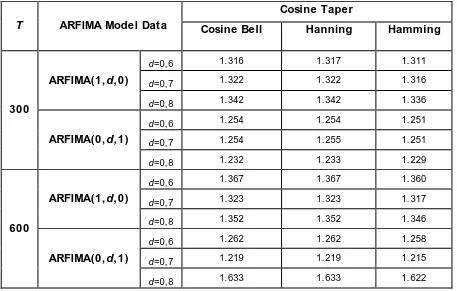
After estimating ARFIMA parameters, we calculate Mean square error of forecasting with the value of out sample h =10. MSE of forecasting could be seen at table 2.

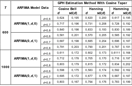
Table 1 Mean and Standard deviation of parameter estimation d from ARFIMA model data.

GPH Est imat ion Method Wit h Cosine Taper

T ARFIMA Model Dat a _{Cosine Bell}

d sd(d)

Hanning

d sd(d)

Hamming

d sd(d)

d=0, 6 0, 624 0, 195 0, 620 0, 200 0, 617 0, 195

d=0, 7 0, 717 0, 196 0, 731 0, 208 0, 728 0, 192

ARFIMA(1,d, 0)

d=0, 8 0, 840 0, 198 0, 833 0, 193 0, 830 0, 189

d=0, 6 0, 581 0, 201 0, 570 0, 205 0, 585 0, 192

d=0, 7 0, 687 0, 198 0, 685 0, 204 0, 696 0, 187

600

ARFIMA(0,d, 1)

d=0, 8 0, 791 0, 203 0, 790 0, 201 0, 787 0, 191

d=0, 6 0, 611 0, 172 0. 602 0, 173 0, 6111 0, 168

d=0, 7 0, 712 0, 178 0, 705 0, 170 0, 716 0, 197

ARFIMA(1,d, 0)

d=0, 8 0, 803 0, 179 0, 815 0, 172 0, 834 0, 202

d=0, 6 0, 598 0, 175 0, 583 0, 174 0, 592 0, 162

d=0, 7 0, 695 0, 172 0, 677 0, 176 0, 687 0, 187

1000

ARFIMA(0,d, 1)

Table 2 MSE of Forecasting ( h = 10)

Cosine Taper

T ARFIMA Model Dat a _{Cosine Bell}

Hanning

Hamming

d=0, 6 1. 316 1. 317 1. 311

d=0, 7 1. 322 1. 322 1. 316

ARFIMA(1,d, 0)

d=0, 8 1. 342 1. 342 1. 336

d=0, 6 1. 254 1. 254 1. 251

d=0, 7 1. 254 1. 255 1. 251

300

ARFIMA(0,d, 1)

d=0, 8 1. 232 1. 233 1. 229

d=0, 6 1. 367 1. 367 1. 360

d=0, 7 1. 323 1. 323 1. 317

ARFIMA(1,d, 0)

d=0, 8 1. 352 1. 352 1. 346

d=0, 6 1. 262 1. 262 1. 258

d=0, 7 1. 219 1. 219 1. 215

600

ARFIMA(0,d, 1)

d=0, 8 1. 633 1. 633 1. 622

5. CONCLUSION

From simulation results, GPH method with Cosine Bell tapering shows a good performance in estimating the differencing parameter of ARFIMA(0,d,1) data. From ARFIMA(1,d,0) data, GPH method with Hanning tapering is the best of all methods. From forecasting result, Mean square error of GPH method with Hamming tapering has the least value of all data types.

6. ACKNOWLEDGEMENTS

REFERENCES

Bisaglia, L and Guegan, Dominique. (1998), “A Comparison of Techniques of estimation in long-memory processes”, Computational Statistics & Data Analysis”, Vol.27, p. 61-81.

Fox, R and Taqqu, M.S. (1986). “Large-sample Properties of Parameter Estimates for Strongly Dependent Stationary Gaussian Time Series”, The Annals of Statistics, Vol.14, p. 517-532. Geweke J and Porter-Hudak,S. (1983), “The Estimation and Application of Long Memory Time Series

Models”, Journal of Time series Analysis,Vol. 4, p. 221-238.

Granger, C. W. J. and Joyeux,R. (1980), “An Introduction to Long-Memory Time Series Models and Fractional Differencing”, Journal of Time Series Analysis, Vol. 1, p. 15-29.

Hosking, J.R.M. (1981), “Fractional Differencing”, Biometrika, Vol. 68, p. 165-176.

Hurvich, C.M. and Deo,R.S. (1999), “An Introduction to Long-Memory Time Series Models and fractional Differencing”, Journal of Time series Analysis, Vol. 20, p.331-341.

Hurvich, C.M. and Ray, B.K. (1995), “Estimation of the Memory Parameter for Non stationary or Noninvertible Fractionally Integrated Processes”, Journal of Time series Analysis, Vol. 16, p.17-42.

Reisen, V.A. (1994), “ Estimation of the Fractional Parameter for ARIMA(p,d,q) Model Using the Smoothed Periodogram”, Journal of Time Series Analysis, Vol.15, p. 335-350.

Reisen, V.A and Lopes,S.R.C. (1999), “Some Simulations and applications of forecasting long-memory time series models”, Journal of Statistical Planning and Inference, Vol.80, p. 269-287.

Robinson, P.M. (1995), “Log-Periodogram Regression of Time Series with Long Range Dependence”, Annals of Statistics, Vol. 23, pp. 1048-1072.

Sowell, F. (1992), “Maximum Likelihood Estimation of Stationary Univariate Fractionally Integrated Time Series Models”, Journal of econometrics, Vol.53, p.165 – 188.

Velasco, C. (1999a), ”Non-Stationary Log-Periodogram Regression”, Journal of Econometric, Vol. 91, p. 325-371.