Series Editors
E.D. Sontag · M. Thoma · A. Isidori · J.H. van Schuppen
Published titles include: Stability and Stabilization of Infinite Dimensional Systems with Applications
Zheng-Hua Luo, Bao-Zhu Guo and Omer Morgul
Nonsmooth Mechanics (Second edition)
Bernard Brogliato
Nonlinear Control Systems II
Alberto Isidori
L2-Gain and Passivity Techniques
in Nonlinear Control
Arjan van der Schaft
Control of Linear Systems with Regulation and Input Constraints
Ali Saberi, Anton A. Stoorvogel and Peddapullaiah Sannuti
Robust and H∞Control
Ben M. Chen
Computer Controlled Systems
Efim N. Rosenwasser and Bernhard P. Lampe
Control of Complex and Uncertain Systems
Stanislav V. Emelyanov and Sergey K. Korovin
Robust Control Design Using H∞Methods
Ian R. Petersen, Valery A. Ugrinovski and Andrey V. Savkin
Model Reduction for Control System Design
Goro Obinata and Brian D.O. Anderson
Control Theory for Linear Systems
Harry L. Trentelman, Anton Stoorvogel and Malo Hautus
Functional Adaptive Control
Simon G. Fabri and Visakan Kadirkamanathan
Positive 1D and 2D Systems
Tadeusz Kaczorek
Identification and Control Using Volterra Models
Francis J. Doyle III, Ronald K. Pearson and Bobatunde A. Ogunnaike
Non-linear Control for Underactuated Mechanical Systems
Isabelle Fantoni and Rogelio Lozano
Learning and Generalization (Second edition)
Mathukumalli Vidyasagar
Constrained Control and Estimation
Graham C. Goodwin, María M. Seron and José A. De Doná
Randomized Algorithms for Analysis and Control of Uncertain Systems
Roberto Tempo, Giuseppe Calafiore and Fabrizio Dabbene
Switched Linear Systems
Zhendong Sun and Shuzhi S. Ge
Subspace Methods for System Identification
Tohru Katayama
Digital Control Systems
Ioan D. Landau and Gianluca Zito
Multivariable Computer-controlled Systems
Efim N. Rosenwasser and Bernhard P. Lampe
Dissipative Systems Analysis and Control (Second edition)
Bernard Brogliato, Rogelio Lozano, Bernhard Maschke and Olav Egeland
Algebraic Methods for Nonlinear Control Systems (Second edition)
Giuseppe Conte, Claude H. Moog and Anna Maria Perdon
Polynomial and Rational Matrices
Tadeusz Kaczorek
Simulation-based Algorithms for Markov Decision Processes
Hyeong Soo Chang, Michael C. Fu, Jiaqiao Hu and Steven I. Marcus
Iterative Learning Control
Hyo-Sung Ahn, Kevin L. Moore and YangQuan Chen
Distributed Consensus in Multi-vehicle Cooperative Control
Wei Ren and Randal W. Beard
Control of Singular Systems with Random Abrupt Changes
El-K´ebir Boukas
Robust Control (Second edition)
Jürgen Ackermann
Flow Control by Feedback
Ole Morten Aamo and Miroslav Krsti´c
Nonlinear and Adaptive Control with Applications
Felix L. Chernousko
·
Igor M. Ananievski
·
Sergey A. Reshmin
Control of Nonlinear
Dynamical Systems
Methods and Applications
F.L. Chernousko
Russian Academy of Sciences Institute for Problems in Mechanics Vernadsky Ave. 101-1
Moscow Russia 119526 [email protected]
S.A. Reshmin
Russian Academy of Sciences Institute for Problems in Mechanics Vernadsky Ave. 101-1
Moscow Russia 119526 [email protected]
I.M. Ananievski
Russian Academy of Sciences Institute for Problems in Mechanics Vernadsky Ave. 101-1
Moscow Russia 119526 [email protected]
ISBN: 978-3-540-70782-0 e-ISBN: 978-3-540-70784-4
DOI: 10.1007/978-3-540-70784-4
Communications and Control Engineering ISSN: 0178-5354
Library of Congress Control Number: 2008932362 c
2008 Springer-Verlag Berlin Heidelberg
This work is subject to copyright. All rights are reserved, whether the whole or part of the material is concerned, specifically the rights of translation, reprinting, reuse of illustrations, recitation, broadcasting, reproduction on microfilm or in any other way, and storage in data banks. Duplication of this publication or parts thereof is permitted only under the provisions of the German Copyright Law of September 9, 1965, in its current version, and permission for use must always be obtained from Springer. Violations are liable to prosecution under the German Copyright Law.
The use of general descriptive names, registered names, trademarks, etc. in this publication does not imply, even in the absence of a specific statement, that such names are exempt from the relevant protective laws and regulations and therefore free for general use.
Cover design:Integra Software Services Pvt. Ltd. Printed on acid-free paper
This book is devoted to new methods of control for complex dynamical systems and deals with nonlinear control systems having several degrees of freedom, subjected to unknown disturbances, and containing uncertain parameters. Various constraints are imposed on control inputs and state variables or their combinations.
The book contains an introduction to the theory of optimal control and the theory of stability of motion, and also a description of some known methods based on these theories.
Major attention is given to new methods of control developed by the authors over the last 15 years. Mechanical and electromechanical systems described by nonlinear Lagrange’s equations are considered. General methods are proposed for an effective construction of the required control, often in an explicit form. The book contains various techniques including the decomposition of nonlinear control systems with many degrees of freedom, piecewise linear feedback control based on Lyapunov’s functions, methods which elaborate and extend the approaches of the conventional control theory, optimal control, differential games, and the theory of stability.
The distinctive feature of the methods developed in the book is that the con-trols obtained satisfy the imposed constraints and steer the dynamical system to a prescribed terminal state in finite time. Explicit upper estimates for the time of the process are given. In all cases, the control algorithms and the estimates obtained are strictly proven.
The methods are illustrated by a number of control problems for various en-gineering systems: robotic manipulators, pendular systems, electromechanical sys-tems, electric motors, multibody systems with dry friction, etc. The efficiency of the proposed approaches is demonstrated by computer simulations.
The authors hope that the monograph will be a useful contribution to the sci-entific literature on the theory and methods of control for dynamical systems. The
book could be of interest for scientists and engineers in the field of applied mathe-matics, mechanics, theory of control and its applications, and also for students and postgraduates.
Moscow, Felix L. Chernousko
April 2008 Igor M. Ananievski
Introduction. . . 1
1 Optimal control. . . 11
1.1 Statement of the optimal control problem . . . 11
1.2 The maximum principle . . . 16
1.3 Open-loop and feedback control . . . 21
1.4 Examples . . . 23
2 Method of decomposition (the first approach) . . . 31
2.1 Problem statement and game approach . . . 31
2.1.1 Controlled mechanical system . . . 31
2.1.2 Simplifying assumptions . . . 32
2.1.3 Decomposition . . . 35
2.1.4 Game problem . . . 36
2.2 Control of the subsystem and feedback control design . . . 37
2.2.1 Optimal control for the subsystem . . . 37
2.2.2 Simplified control for the subsystem . . . 42
2.2.3 Comparative analysis of the results . . . 45
2.2.4 Control for the initial system . . . 52
2.3 Weak coupling between degrees of freedom . . . 54
2.3.1 Modification of the decomposition method . . . 54
2.3.2 Analysis of the controlled motions . . . 56
2.3.3 Determination of the parameters . . . 59
2.3.4 Case of zero initial velocities . . . 61
2.4 Nonlinear damping . . . 67
2.4.1 Subsystem with nonlinear damping . . . 67
2.4.2 Control for the nonlinear subsystem . . . 69
2.4.3 Simplified control for the subsystem and comparative analysis . . . 74
2.5 Applications and numerical examples . . . 82
2.5.1 Application to robotics . . . 82
2.5.2 Feedback control design and modelling of motions for
two-link manipulator with direct drives . . . 86
2.5.3 Modelling of motions of three-link manipulator . . . 92
3 Method of decomposition (the second approach). . . 103
3.1 Problem statement and game approach . . . 103
3.1.1 Controlled mechanical system . . . 103
3.1.2 Statement of the problem . . . 105
3.1.3 Control in the absence of external forces . . . 106
3.1.4 Decomposition . . . 108
3.2 Feedback control design and its generalizations . . . 112
3.2.1 Feedback control design . . . 112
3.2.2 Control in the general case . . . 114
3.2.3 Extension to the case of nonzero terminal velocity . . . 117
3.2.4 Tracking control for mechanical system . . . 124
3.3 Applications to robots . . . 131
3.3.1 Symbolic generation of equations for multibody systems . . . 131
3.3.2 Modelling of control for a two-link mechanism (with three degrees of freedom) . . . 136
3.3.3 Modelling of tracking control for a two-link mechanism (with two degrees of freedom) . . . 144
4 Stability based control for Lagrangian mechanical systems . . . 147
4.1 Scleronomic and rheonomic mechanical systems . . . 147
4.2 Lyapunov stability of equilibrium . . . 151
4.3 Lyapunov’s direct method for autonomous systems . . . 151
4.4 Lyapunov’s direct method for nonautonomous systems . . . 153
4.5 Stabilization of mechanical systems . . . 153
4.6 Modification of Lyapunov’s direct method . . . 155
5 Piecewise linear control for mechanical systems under uncertainty. . . 157
5.1 Piecewise linear control for scleronomic systems . . . 157
5.1.1 Problem statement . . . 157
5.1.2 Description of the control algorithm . . . 159
5.1.3 Justification of the algorithm . . . 161
5.1.4 Estimation of the time of motion . . . 166
5.1.5 Sufficient condition for steering the system to the prescribed state . . . 168
5.2 Applications to mechanical systems . . . 170
5.2.1 Control of a two-link manipulator . . . 170
5.2.2 Control of a two-mass system with unknown parameters . . . 173
5.2.3 The first stage of the motion . . . 178
5.2.4 The second stage of the motion . . . 182
5.2.5 System “a load on a cart” . . . 186
5.2.7 Computer simulation results . . . 197
5.3 Piecewise linear control for rheonomic systems . . . 199
5.3.1 Problem statement . . . 199
5.3.2 Control algorithm for rheonomic systems . . . 200
5.3.3 Justification of the control . . . 201
5.3.4 Results of simulation . . . 210
6 Continuous feedback control for mechanical systems under uncertainty. . . 213
6.1 Feedback control for scleronomic system with a given matrix of inertia . . . 213
6.1.1 Problem statement . . . 213
6.1.2 Control function . . . 214
6.1.3 Justification of the control . . . 217
6.1.4 Sufficient condition for controllability . . . 222
6.1.5 Computer simulation results . . . 223
6.2 Control of a scleronomic system with an unknown matrix of inertia 229 6.2.1 Problem statement . . . 229
6.2.2 Computer simulation of the motion of a two-link manipulator234 6.3 Control of rheonomic systems under uncertainty . . . 237
6.3.1 Problem statement . . . 237
6.3.2 Computer simulation results . . . 241
7 Control in distributed-parameter systems. . . 245
7.1 System of linear oscillators . . . 245
7.1.1 Equations of motion . . . 245
7.1.2 Decomposition . . . 246
7.1.3 Time-optimal control problem . . . 248
7.1.4 Upper bound for the optimal time . . . 249
7.2 Distributed-parameter systems . . . 252
7.2.1 Statement of the control problem for a distributed-parameter system . . . 252
7.2.2 Decomposition . . . 254
7.2.3 First-order equation in time . . . 257
7.2.4 Second-order equation in time . . . 258
7.2.5 Analysis of the constraints and construction of the control . . 259
7.3 Solvability conditions . . . 263
7.3.1 The one-dimensional problems . . . 263
7.3.2 Control of beam oscillations . . . 266
7.3.3 The two-dimensional and three-dimensional problems . . . 267
8 Control system under complex constraints. . . 275
8.1 Control design in linear systems under complex constraints . . . 275
8.1.1 Problem statement . . . 275
8.1.2 Kalman’s approach . . . 277
8.2 Application to oscillating systems . . . 281
8.2.1 Control for the system of oscillators . . . 281
8.2.2 Pendulum with a suspension point controlled by acceleration 286 8.2.3 Pendulum with a suspension point controlled by acceleration (continuation) . . . 290
8.2.4 Pendulum with a suspension point controlled by velocity . . . 296
8.3 Application to electro-mechanical systems . . . 303
8.3.1 Model of the electro-mechanical system . . . 303
8.3.2 Analysis of the simplified model . . . 306
8.3.3 Control of the electro-mechanical system of the fourth order 310 8.3.4 Active dynamical damper . . . 317
9 Optimal control problems under complex constraints . . . 327
9.1 Time-optimal control problem under mixed and phase constraints . . 328
9.1.1 Problem statement . . . 328
9.1.2 Time-optimal control under constraints imposed on the velocity and acceleration . . . 329
9.1.3 Problem of control of an electric motor . . . 335
9.2 Time-optimal control under constraints imposed on the rate of change of the acceleration . . . 340
9.2.1 Statement of the problem . . . 340
9.2.2 Open-loop optimal control . . . 342
9.2.3 Feedback optimal control . . . 345
9.3 Time-optimal control under constraints imposed on the acceleration and its rate . . . 354
9.3.1 Problem statement . . . 354
9.3.2 Possible modes of control . . . 357
9.3.3 Construction of the trajectories . . . 359
10 Time-optimal swing-up and damping feedback controls of a nonlinear pendulum. . . 367
10.1 Optimal control structure . . . 368
10.1.1 Statement of the problem . . . 368
10.1.2 Phase cylinder . . . 369
10.1.3 Maximum principle . . . 370
10.1.4 Numerical algorithm . . . 371
10.2 Swing-up control . . . 372
10.2.1 Literature overview . . . 372
10.2.2 Special trajectories . . . 373
10.2.3 Numerical results . . . 375
10.3.1 Literature overview . . . 380
10.3.2 Special trajectories . . . 382
10.3.3 Numerical results . . . 383
References . . . 389
Introduction
There exist numerous methods for the design of control for dynamical systems. The classical methods of the theory of automatic control are meant for linear systems and represent the control in the form of a linear operator applied to the current phase state of the system. Shortcomings of this approach are obvious both in the vicinity of the prescribed terminal state as well as far from it. Near the terminal state, the magnitude of the control becomes small, so that control possibilities are not fully realized. As a result, the time of the control process occurs to be, strictly speaking, infinite, and the phase state can only tend asymptotically to the terminal state as time goes to infinity. On the other hand, far from the terminal state, the control magnitude becomes large and can violate the constraints usually imposed on the control. That is why it is difficult and often impossible to take account of the constraints imposed when the linear methods are used. Moreover, the classical methods based on linear models are usually inapplicable to nonlinear systems; at least, their applicability should be justified thoroughly.
In principle, the methods of the theory of optimal control can be applied to non-linear systems. These methods take account of various constraints imposed on the control and, though with considerable complications, on the state variables. The methods of optimal control bring a dynamical system to a prescribed terminal state in an optimal (in a certain sense) way; for example, in a minimum time. However, to construct the optimal control for a nonlinear system is a very complicated problem, and its explicit solution is seldom available. Especially difficult is the construction of a feedback optimal control for a nonlinear system, even for a system with a small number of degrees of freedom and even with the help of modern computers.
There exist a number of other general methods of control: the method of systems with variable structure [123, 116, 115], the method of feedback linearization [70, 71, 91], and their various generalizations. However, these methods usually do not take into account constraints imposed on the control and state variables. Moreover, being very general, these methods do not take account of specific properties of mechanical systems such as conservation laws or the structure of basic equations of motions that can be presented in the Lagrangian or the Hamiltonian forms. Some other control
methods applicable to nonlinear mechanical systems were developed in [61, 62, 94, 95, 59, 51, 52, 85, 90, 118].
In this book, some methods of control for nonlinear mechanical systems sub-jected to perturbations and uncertainties are proposed. These methods are applicable in the presence of various constraints on control and state variables. By taking into account some specific properties inherent in the equations of mechanical systems, these methods yield more efficient control algorithms compared with the methods developed for general systems of differential equations.
The authors’ objective was to develop control methods having the following fea-tures.
1. Methods are applicable to nonlinear mechanical systems described by the La-grange equations.
2. Methods are applicable to systems with many degrees of freedom.
3. Methods take into account the constraints imposed on the control, and, in a number of cases, also on the state variables as well as on both the control and state variables.
4. Methods bring the control system to the prescribed terminal state in finite time, and an efficient upper estimate is available for this time.
5. Methods are applicable in the presence of uncertain but bounded external per-turbations and uncertain parameters of the system. Thus, the methods are robust.
6. There exist efficient algorithms for the construction of the desired feedback control.
7. Efficient sufficient controllability conditions are stated for the control methods proposed.
8. In all cases, a rigorous mathematical justification of the proposed methods is given.
It is clear that the above requirements are very useful and important from the standpoint of the control theory as well as various practical applications.
Several methods are proposed and developed in the book, and not all of them possess all of the features 1–8 listed above. Properties 3, 4, 7, and 8 are always fulfilled, whereas other features are inherent in some of the methods and not present in others.
The book consists of 10 chapters.
Chapters 2, 3, 5, and 6 deal with nonlinear mechanical systems with many de-grees of freedom governed by Lagrange’s equations and subjected to control and perturbation forces.
These equations are taken in the form:
d dt
∂T
∂q˙i−
∂T
∂qi
=Ui+Qi, i=1, . . . ,n. (0.1)
Here,t is time, the dots denote time derivatives, qi are the generalized
coordi-nates, ˙qiare the generalized velocities,Uiare the generalized control forces,Qiare
is a symmetric positive definite quadratic form of the generalized velocities ˙qi:
T(q,q˙) =1
2A(q)q,˙ q˙= 1 2
n
∑
j,k=1ajk(q)q˙jq˙k. (0.2)
Here,q and ˙q are then-vectors of the generalized coordinates and velocities, respectively, and the brackets·,·denote the scalar product of vectors.
The quadratic form (0.2) satisfies the conditions
m|q˙|2≤ A(q)q,˙ q˙ ≤M|q˙|2 (0.3)
for anyq∈Rnand ˙q∈Rn, wheremandMare positive constants such thatM>m. Condition (0.3) implies that all eigenvalues of the matrixA(q), for allq∈Rn, belong to the interval[m,M].
In Chapters 2 and 3, the coefficients of the quadratic form (0.2) are supposed to be known functions of the coordinates:ajk=ajk(q). In Chapters 5 and 6, the functions
ajk(q)may be unknown but the constantsmandMin (0.3) are given. Also, the case
of rheonomic systems for whichT =T(q,q,˙ t)is considered in Chapter 5.
We suppose that the control forces are subjected to the geometric constraints at any time instant:
|Ui| ≤Ui0, i=1, . . . ,n, (0.4)
whereUi0are given constants.
The generalized forces Qi may be more or less arbitrary functions of the
co-ordinates, velocities, and time; these functions may be unknown but are assumed bounded by the inequality
|Qi(q,q,˙ t)| ≤Q0i, i=1, . . . ,n, (0.5)
The constantsQ0i are supposed to be known, and certain upper bounds are im-posed onQ0i in order to achieve the control objective.
The control problem is formulated as follows:
Problem 0.1.It is required to construct the feedback controlUi(q,q˙) that brings
system (0.1) subject to constraints (0.3)–(0.5) from the given initial state
q(t0) =q0, q˙(t0) =q˙0 (0.6)
at a given initial time instantt=t0to the prescribed terminal state with zero terminal
generalized velocities
q(t∗) =q∗, q˙(t∗) =0 (0.7) in finite time. The time instantt∗is not prescribed but an upper estimate on it should be obtained.
In some sections of Chapter 3, the case of nonzero terminal velocities ˙qi(t∗)=0
In many practical applications, it is desirable to bring the system from the state (0.6) to the state (0.7) as soon as possible, i.e., to minimizet∗. However, to construct the exact solution of this time-optimal control problem for the nonlinear system is a very difficult problem, especially, if one desires to obtain the feedback control. The methods proposed in Chapters 2, 3, and 5–8 do not provide the time-optimal control but include certain procedures of optimization of the time t∗. Therefore, these methods may sometimes be called suboptimal.
The main difficulties arising in the construction of the control for system (0.1) are due to its nonlinearity and its high order. The complex nonlinear dynamical interac-tion of different degrees of freedom of the system is characterized by the elements
ajk(q)of the matrixA(q)of the kinetic energy. Another property that complicates
the construction of the control is the fact that the dimensionnof the control vector is two times less than the order of system (0.1).
Manipulation robots can be regarded as typical examples of mechanical or elec-tromechanical systems described by equations (0.1). Being an essential part of au-tomated manufacturing systems, these robots can serve for various technological operations. A manipulation robot is a controlled mechanical system that consist of one or several manipulators, a control system, drives (actuators), and grippers. A manipulator can perform a wide range of three-dimensional motions and bring ob-jects (instruments and/or workpieces) to a prescribed position and orientation in space. Various types of drives, namely, electric, hydraulic, pneumatic, and other, are employed in robotic manipulators, the electric drives being the most widespread.
The manipulator is a multibody system that consists of several links connected by joints. The drives are usually located at the joints or inside links adjacent to the joints. Relative angular or linear displacements of neighboring links are usu-ally chosen as the generalized coordinatesqiof the manipulator. The kinetic energy
T(q,q˙)of the manipulator consists of the kinetic energy of its links and also, if the drives are taken into account, the kinetic energy of electric drives and gears. The Lagrange equations (0.1) of the manipulator involve the generalized forcesQi
due to the weight and resistance forces; the latter are often not known exactly and may change during operations. Moreover, parameters of the manipulator may also change in an unpredictable way. Therefore, some of the forcesQishould be regarded
as uncertain perturbations. The control forcesUiare forces and/or torques produced
by the drives.
Since the manipulator is a nonlinear multibody system subject to uncertain per-turbations, it is quite natural to consider the problem of control for the manipulator as a nonlinear control problem formulated above as Problem 0.1.
Let us outline briefly the contents of Chapters 1–10.
Chapter 1 gives an introduction to the theory of optimal control. Basic concepts and results of this theory, especially the Pontryagin maximum principle, are often used throughout the book. The maximum principle is formulated and illustrated by several examples. The feedback optimal controls obtained for these examples are often referred to in the following chapters.
nonlinear system (0.1) withndegrees of freedom to the set ofnindependent linear subsystems
¨
xi=ui+vi, i=1, . . . ,n. (0.8)
Here,xiare the new (transformed) generalized coordinates,uiare the new controls,
and forcesviinclude the generalized forcesQi, as well as the nonlinear terms that
describe the interaction of different degrees of freedom in system (0.1). The pertur-bationsviin system (0.8) are treated as uncertain but bounded forces; they can also
be regarded as the controls of another player that counteract the controlsui.
The original constraints (0.3)–(0.5) imposed on the kinetic energy and general-ized forces of system (0.1) are, under certain conditions, reduced to the following normalized constraints on controlsuiand disturbancesvi:
|ui| ≤1, |vi| ≤ρi, ρi<1, i=1, . . . ,n. (0.9)
By applying the approach of differential games [69, 79] to system (0.8) subject to constraints (0.9), we obtain the feedback controlui(xi,x˙i)that solves the control
problem for theith subsystem, ifρi<1.
Besides the game-theoretical technique, a simpler approach to the control con-struction is also considered, where the perturbations in system (0.8) are completely ignored. As the control ui(xi,x˙i) of the ith subsystem (0.8) we choose the
time-optimal feedback control for the system
¨
xi=ui, i=1, . . . ,n.
It is shown that this simplified approach is effective, i.e., brings theith subsystem (0.8) to the prescribed terminal state, if and only if the numberρiin (0.9) does not
exceed the golden section ratio:
ρi<ρ∗=
1 2(
√
5−1)≈0.618.
In other words, uncertain but bounded perturbations can be neglected while con-structing the feedback control, if and only if their magnitude divided by the magni-tude of the control does not exceed the golden section ratioρ∗.
Two versions of the decomposition method presented in Chapters 2 and 3 differ both by the assumptions made and the results obtained.
The assumptions of the second version (Chapter 3) are less restrictive; on the other hand, the time of the control process is usually less for the first version (Chap-ter 2).
As a result of each decomposition method, explicit feedback control laws for the original system (0.1) are obtained. These control lawsUi=Ui(q,q˙),i=1, . . . ,n,
satisfy the imposed constraints (0.4) and bring the system to the terminal state (0.7) under any admissible perturbationsQi(q,q,t˙ )subject to conditions (0.5). Sufficient
controllability conditions are derived for the methods proposed. The time of control
Certain generalizations and modifications of the decomposition methods are pre-sented in Chapters 2 and 3. The original system (0.1) withndegrees of freedom can be reduced to sets of subsystems more complicated than (0.8); these subsystems can be either linear or nonlinear, and these two cases are examined. The decompo-sition method is extended to the case of nonzero prescribed terminal velocity ˙qi(t∗)
in (0.7), and also to the problem of tracking the prescribed trajectory of motion. Control problems for the manipulation robots with several degrees of freedom are considered as examples illustrating the methods proposed. Purely mechanical models of robots as well as electromechanical models that take account of processes in electric circuits are considered.
Chapter 4 briefly presents basic concepts and results of the theory of stability. Here, the notion of the Lyapunov function plays the central role, and the corre-sponding theorems using this notion are formulated. The Lyapunov functions are widely used in the following Chapters 5 and 6.
In these chapters, the method of control based on the piecewise linear feedback for system (0.1)–(0.7) is presented. The required control vectorU is sought in the form
U=−β(q−q∗)−αq,˙ U= (U1, . . . ,Un), (0.10)
whereα andβ are scalar coefficients.
During the motion, the coefficients increase in accordance with a certain algo-rithm and may tend to infinity as the system approaches the terminal state (0.7), i.e.,t→t∗. However, the control forces (0.10) stay bounded and satisfy the imposed constraints (0.4).
In Chapter 5, the coefficientsαandβ are piecewise constant functions of time. These coefficients change when the system reaches certain prescribed ellipsoidal surfaces in 2n-dimensional phase space. In Chapter 6, the coefficientsα andβ are continuous functions of time.
In both Chapters 5 and 6, the proposed algorithms are rigorously justified with the help of the second Lyapunov method. It is proven that this control technique brings the system (0.1) to the prescribed terminal state (0.7) in finite time. An explicit upper bound for this time is obtained.
The methods of Chapters 5 and 6 are applicable not only in the case of uncertain perturbations satisfying (0.5), but also if the matrixAof the kinetic energy (0.2) is uncertain. It is only necessary that restrictions (0.3) hold and the constantsmandM
be known.
The approach based on the feedback control (0.10) is extended also to rheonomic systems whose kinetic energy is a second-order polynomial of the generalized ve-locities with coefficients depending explicitly on the generalized coordinates and time (Chapter 5). The coefficients of the kinetic energy are assumed unknown, and the system is acted upon by uncertain perturbations. The control algorithm is given that brings the rheonomic system to the prescribed terminal state by a bounded con-trol force.
and friction, are assumed unknown, and uncertain perturbations are also taken into account. It is shown that the methods proposed in Chapters 5 and 6 can control such systems and bring them to the terminal state; moreover, the methods are efficient even if the sufficient controllability conditions derived in Chapters 5 and 6 are not satisfied.
Note that, together with the methods discussed in the book, there are other ap-proaches that ensure asymptotic stability of a given state of the system, i.e., bring the system to this state ast→∞. In practice, one needs to bring the system to the vicinity of the prescribed state; therefore, the algorithms based on the asymptotic stability practically solve the control problem in finite time. However, as the re-quired vicinity of the terminal state decreases and tends to zero, the time of motion for the control methods ensuring the asymptotic stability increases and tends to in-finity. By contrast, the methods proposed in this book ensure that the time of motion is finite, and explicit upper bounds for this time are given in Chapters 2, 3, 5, and 6. In Chapters 1–6, systems with finitely many degrees of freedom are considered; these are described by systems of ordinary differential equations. A number of books and papers (see, for example, [25, 122, 86, 113, 117, 87]) are devoted to control problems for systems with distributed parameters that are described by partial dif-ferential equations. The methods of decomposition proposed in Chapters 2 and 3 can also be applied to systems with distributed parameters.
In Chapter 7, control systems with distributed parameters are considered. These systems are described by linear partial differential equations resolved with respect to the first or the second time derivative. The first case corresponds, for example, to the heat equation, and the second to the wave equation. The control is supposed to be distributed and bounded; it is described by the corresponding terms in the right-hand side of the equation. The control problem is to bring the system to the zero terminal state in finite time. The proposed control method is based on the decomposition of the original system into subsystems with the help of the Fourier method. After that, the time-optimal feedback control is applied to each mode. A peculiarity of this control problem is that there is an infinite (countable) number of modes.
Sufficient controllability conditions are derived. The required feedback control is obtained, together with upper estimates for the time of the control process. These results are illustrated by examples.
In Chapters 8–10, we return to control systems governed by ordinary differential equations.
In Chapter 8, we consider linear systems subject to various constraints. Control and phase constraints, as well as mixed constraints imposed on both the control and the state variables are considered. Integral constraints on control and state variables are also taken into account. Though the original systems are linear, the presence of complex constraints makes the control problem essentially nonlinear and rather complicated.
control torque, and also on their combination. Integral constraints typically occur, if there are energy restrictions.
The approach developed in Chapter 8 is a generalization of the well-known Kalman’s method [72, 73]. This method, originally proposed for the control of linear systems in the absence of constraints, is based on the representation of the control as a linear combination of the eigenmodes of motion. In Chapter 8, this method is extended to some cases with different constraints. Explicit control laws are ob-tained for various oscillatory systems, in particular, a system of many oscillators controlled by one bounded control. For certain systems of the second order, the controls obtained are compared with time-optimal controls. The method is applied also to systems of the fourth (and higher) order with mixed constraints. The models considered here correspond to mechanical and electromechanical systems contain-ing an oscillator and an electric motor. Sufficient controllability conditions derived in Chapter 8 ensure that the control obtained brings the system to the prescribed state in finite time, and all mixed constraints are satisfied.
Chapter 9 is devoted to several control problems for a simple dynamical system with one degree of freedom described by the second Newton’s law and subject to different constraints that model real constraints typical for actuators. The system is to be brought to the origin of the coordinate system in the phase plane.
First, the time-optimal control problem is considered in the presence of mixed constraints imposed on the control and state variables. The time-optimal feedback control is obtained. As an example, a control problem for the electric drive is exam-ined.
Next, a constraint is imposed on the rate of change of the control force. Such a constraint is often inherent in various drives. The resultant equations are reduced to a third-order system. The time-optimal control problem for this system is solved, and the required control is obtained in the open-loop as well as in the feedback form. The solution of this problem is based on a group-invariant approach that reduces the number of the essential phase variables from three to two.
At the end of Chapter 9, it is supposed that the absolute value of the control force can grow only gradually, with a bounded rate, whereas this force can be switched off instantly. Under these assumptions, which model real drives, we find the control that brings the system to a prescribed state and has the simplest possible structure.
mathematical proof is given, and a number of specific control problems are analyzed and solved by these methods.
Optimal control
In the following chapters of the book we will often use the approach and concepts of the optimal control theory. Also, some of the proposed methods of control utilize certain results obtained for particular optimal control problems and use these results as integral parts of our control algorithms. Thus, it would be useful to recall the basic concepts of the optimal control theory and describe the solution of several typical problems.
1.1 Statement of the optimal control problem
We consider a general dynamical system subjected to control and described by the following nonlineardifferential equation
˙
x=f(x,u,t). (1.1.1)
Here,x= (x1, . . . ,xn)is then-dimensional vector of state andu= (u1, . . . ,um)is
them-dimensional vector of control; these vectors are functions of timet:x=x(t),
u=u(t). The dot.denotes differentiation with respect to time. Then-dimensional vector f(x,u,t)is a given function of its arguments. Equation (1.1.1) is sometimes calledequation of motion.
Control systems can also be described by more general classes of equations: ferential algebraic equations (DAE), integro-differential equations, functional dif-ferential equations, etc. In this book, we mostly restrict ourselves to difdif-ferential equations (1.1.1).
To formulate the optimal control problem, we should, in addition to (1.1.1), im-poseboundary conditions, constraints, and anoptimality criterion, or acost func-tional. The control process is considered on the time intervalt∈[t0,T], the endst0
andT of this interval may be fixed or free.
In general, theboundary conditionscan be stated as follows:
(t0,x(t0))∈X0, (T,x(T))∈XT, (1.1.2)
whereX0andXT are given sets in the(n+1)-dimensional(t,x)-space.
Let us restrict ourselves to the case mostly considered in this book, where the initial data are fixed so that the setX0in (1.1.2) is a given point(t0,x0)in the(t,x)
-space. Hence, we have the initial condition
x(t0) =x0. (1.1.3)
Here, the time instantt0and the vectorx0are fixed.
We assume also that the setXT in (1.1.2) is defined byrequations in thex-space
XT ={t=T,x:gi(x) =0}, i=1, . . . ,r≤n, (1.1.4)
whereas the terminal timeTmay be either fixed or free. Here,gi(x)are given scalar
functions ofxsuch that the Jacobian matrix
G=
∂gi
∂xj
, i=1, . . . ,r, j=1, . . . ,n, (1.1.5)
has the maximal possible rankron the set defined by (1.1.4).
The simplest case of the conditions (1.1.2) often referred to in this book is the so-calledtwo-point boundary conditionswhere both vectorsx(t0)andx(T)are fixed.
In this case, in addition to (1.1.3) we have
x(T) =x1, (1.1.6)
wherex1is a given vector. The terminal timeT may be fixed or free. Note that in the case of (1.1.6) we have
gi=xi−x1i, i=1, . . . ,n, r=n, G=I,
in (1.1.4) and (1.1.5), whereIis the identity matrix.
Constraintsmay be imposed on the controlu, the statex, or both.Control con-straintsare often expressed in the form
u(t)∈U, t∈[t0,T], (1.1.7)
whereUis a given closed set in them-dimensionalu-space.
State constraintscan be expressed in a similar way
x(t)∈V, t∈[t0,T], (1.1.8)
whereV is a given closed set in then-dimensionalx-space.
Both sets in (1.1.7) and (1.1.8) may depend on time so that we haveU=U(t)and
V =V(t). Note that the boundary conditions (1.1.2) can be formally considered as a particular case of the state constraints imposed at two specific time instantst=t0
In more general [than (1.1.7) and (1.1.8)] case ofmixed constraints, we have
u(t)∈U(x(t),t), t∈[t0,T], (1.1.9)
whereU(x,t)is, for allxandt∈[t0,T], a closed set in them-dimensionalu-space;
this set depends onxandt. The constraint (1.1.9) can be also expressed as follows:
(u(t),x(t))∈W(t), t∈[t0,T]. (1.1.10)
Here,W(t)is, for anyt∈[t0,T], a closed set in the(m+n)-dimensional(u,x)-space.
All constraints described by (1.1.7)–(1.1.10) are sometimes called geometric; they are imposed on the values of the control and state at any given instantt.
Another class of constraints areintegral constraintsthat can be imposed on con-trol and state variables. These constraints can be either of equality or inequality type, and the integrals can be taken over either a fixed or variable time interval.
Integral constraints can be often reduced to the boundary conditions and geo-metric state constraints. As an example, let us consider two integral constraints: an equality type constraint with a fixed interval of integration and an inequality type constraint with a variable integration interval. We have
T
t0
ϕ1(x(t),u(t),t)dt=c1,
t
t0
ϕ2(x(τ),u(τ),τ)dτ≥c2(t), t∈[t0,T],
(1.1.11)
whereϕ1andϕ2are given functions,c1is a constant, andc2is a given function of
t.
We introduce additional state variablesxn+i defined by the following equations
and boundary conditions
˙
xn+i=ϕi(x,u,t), xn+i(t0) =0, i=1,2.
Then our integral constraints (1.1.11) can be rewritten as follows:
xn+1(T) =c1, xn+2(t)≥c2(t), t∈[t0,T].
Thus our integral constraints (1.1.11) are reduced to the boundary condition for
xn+1(T)and the state constraint imposed onxn+2(t).
The cost functional, or the optimality criterion, is mostly given as a function depending on the terminal values of the state variables and time
J=F(x(T),T) (1.1.12)
J= T
t0
f0(x(t),u(t),t)dt. (1.1.13)
Here,F(x,t)andf0(x,u,t)are given functions of their arguments. Each type of the
functionals (1.1.12) and (1.1.13) can be reduced to the other one.
If the original functional is given in the terminal form (1.1.12), we introduce the function
f0(x,u,t) =∂
F
∂t + ∂F
∂x,f(x,u,t)
. (1.1.14)
Here,∂/∂xdenotes the vector of gradient, and brackets., .denote the scalar product of vectors.
Then, taking into account (1.1.1), (1.1.3), and (1.1.14), we reduce the terminal functional (1.1.12) to the integral one
J=
T
t0
f0(x,u,t)dt+const.
Vice versa, if we have an integral functional (1.1.13), we introduce an additional state variable by the following equation and initial condition
˙
x0=f0(x,u,t), x0(t0) =0
and express our functional (1.1.13) in the terminal form
J=x0(T).
Also, combinations of terminal and integral functionals can be considered as the optimality criteria; these combinations can be also reduced to one of the basic types (1.1.12) or (1.1.13).
More complicated example of the cost functional is the minimum (or maximum) of some given functionψ(x,t)over the time interval[t0,T], i.e.,
J=min
t ψ(x(t),t), t∈[t0,T]. (1.1.15)
In general, this kind of the functional cannot be reduced to the conventional types (1.1.12) and (1.1.13). However, this reduction is possible, if the derivative
dψ
dt =
∂ ψ ∂t +
∂ ψ
∂x,f(x,u,t)
=g(x,t)
does not depend onu, and the functionψ(x(t),t)has only one minimum with respect tot∈[t0,T]. Then our functional (1.1.15) can be expressed as follows:
whereτis the new terminal time, and the following terminal boundary condition
g(x(τ),τ) =0 should be imposed onτandx(τ).
In this book, we will not deal with cost functionals of the type presented by (1.1.15).
Now we can formulate the optimal control problem in general terms.
For the given system, find thecontrol u(t)and the correspondingstate trajectory x(t)such that they provide the minimal possible value of theoptimality criterion J
under the imposedboundary conditionsandconstraints.
We will always take the system in the form (1.1.1) and impose initial and terminal conditions in one of the forms (1.1.2)–(1.1.4) or (1.1.6). The constraints will be imposed in one of the forms (1.1.7)–(1.1.10), whereas the cost functionalJwill be given by (1.1.12) or (1.1.13).
Without loss of generality, we will always deal with the minimization of the cost functionalJ. If we are interested in the maximization of the functionalJ, it is sufficient just to change the sign of the functional and minimize(−J).
The controlu(t)and state x(t)as the functions of time that correspond to the minimal possible value of the functionalJare called theoptimal controlandoptimal state trajectory, respectively.
The problem of optimal control formulated above is very important for numer-ous practical applications. In particular, this problem arises naturally in control of such mechanical and electromechanical systems as various vehicles (aircraft and spacecraft, rockets, automobiles, ships, and other transport systems), industrial and mobile robots, motors, machines, machine tools, etc. In these applications, the state variablesxi,i=1, . . . ,n, are usually generalized coordinates and velocities of the
mechanical part of the system under consideration as well as electric currents in the electric part of the system. The variablesui,i=1, . . . ,m, denoted usually
con-trol forces and torques, electric voltages, and other concon-trols acting upon the system. The boundary conditions and constraints reflect real limitations and bounds imposed upon the system under consideration.
For example, if u is the thrust acting upon the aircraft, the constraint (1.1.7) expresses the bounds upon the magnitude and direction of the thrust. Since these bounds may depend on the altitude and velocity of the aircraft, we come to the condition (1.1.9), where the setUat any instanttdepends on the current statex(t). Integral constraints (1.1.11) may reflect bounds imposed upon the energy or fuel expenditure. The cost functional (1.1.12) can be related to the desired position and velocity at the terminal state of the aircraft, whereas the integral functional (1.1.13) can be the measure of the fuel or energy consumption.
An important particular case of the optimality criterionJis the time of the control process. This case can be considered, if we put F =T in (1.1.12) or f0=1 in
1.2 The maximum principle
In this section, we will formulate the maximum principle for a class of optimal control problems. This principle was first stated and proved by Pontryagin and his colleagues [93]. Comprehensive information and complete proofs of the maximum principle can be found in numerous books; see, for example, [19, 24, 84, 83].
We consider the system (1.1.1) under the initial condition (1.1.3), terminal con-dition (1.1.4), control constraint (1.1.7), and the cost functional (1.1.13). Thus, our optimal control problem is determined by the following set of equations and condi-tions
˙
x= f(x,u,t), x(t0) =x0, t∈[t0,T],
gi(x(T)) =0, i=1, . . . ,r≤n, u(t)∈U,
J=
T
t0
f0(x(t),u(t),t)→min.
(1.2.1)
The functionsf andf0as well as their first derivatives with respect toxi,i=1, . . . ,n,
are assumed to satisfy the Lipschitz conditions with respect toxandu. The functions
gi, i=1, . . . ,r, are smooth, and the rank of the matrixGfrom (1.1.5) at the set
defined by (1.1.4) is equal tor. The setUin (1.2.1) is a closed set inRm. We will consider two cases: the terminal timeT is either fixed or free.
The controlu(t)will be calledadmissible, if it is a piecewise continuous function oftfort∈[t0,T]and satisfies the constraintu(t)∈Ufor allt∈[t0,T].
The admissible controlu(t)is calledoptimal, if it corresponds to the minimal possible value of the cost functionalJamong all admissible controls.
Suppose the optimal control exists. If we substitute it into our equation of motion and integrate this equation subject to the given initial condition [see (1.2.1)], we obtain theoptimal state trajectory x(t).
Let us introduce the additional state variablex0defined by the following
differ-ential equation and initial condition
˙
x0=f0(x,u,t), x0(t0) =0. (1.2.2)
Then our functionalJfrom (1.2.1) can be expressed asJ=x0(T).
We introduce now the(n+1)-dimensionaladjoint, orconjugate, vector with the components
¯
p(t) = (p0,p1, . . . ,pn) (1.2.3)
and theHamiltonian Hdefined by
H(p,¯ x,u,t) = n
∑
i=0pifi(x,u,t) =p0f0+p,f. (1.2.4)
Note that our equation of motion from (1.2.1) together with (1.2.2) can be rewrit-ten in terms of the Hamiltonian (1.2.4) as follows:
˙
xi=
∂H
∂pi
, i=0,1, . . . ,n. (1.2.5)
The components of the adjoint vector (1.2.3) will obey the following differential equations
˙
pi=−
∂H
∂xi
, i=0,1, . . . ,n. (1.2.6)
Hence, the variablesxiandpi,i=0,1, . . . ,n, satisfy the system of Hamiltonian
equations (1.2.5) and (1.2.6). The componentsxi of the state vector and the
ad-joint variablespiplay the role of the coordinates and impulses, respectively, of the
Hamiltonian system.
Now we can formulate the maximum principle that is a necessary optimality condition. We consider both cases: of the fixed or free terminal timeT.
Theorem 1.1.Let u(t)be an optimal control for the problem defined by (1.2.1) and
x(t)be the corresponding optimal trajectory. Then there exists a nonzero adjoint vectorp¯(t)satisfying the adjoint system (1.2.6) and such that
1)
H(p¯(t),x(t),u(t),t) =sup
u∈U
H(p¯(t),x(t),u,t) (1.2.7)
for t∈[t0,T];
2)
p0=const≤0; (1.2.8)
3) the following boundary conditions hold
pi(T) = r
∑
j=1λj
∂gj(x(T))
∂xi
, i=1, . . . ,n, (1.2.9)
whereλjare constants;
4) if the terminal time T is free, then
H(p¯(T),x(T),u(T),T) =0. (1.2.10)
The proof of Theorem 1.1 can be found in books [93, 19, 24, 84, 83]. We will restrict ourselves only with comments on this theorem.
Conditions (1.2.9) are called thetransversality conditions. They are absent in the case of the two-point problem where the boundary conditions are given by (1.1.3) and (1.1.6). In this case, we haver=n, and the number of unknown constantsλiis
equal to the number of equations (1.2.9), so that these equations do not provide any additional conditions.
If the closed setUis bounded, then the upper bound ofHoveru∈U in (1.2.7) is attained, and this equation implies
u(t) =arg max
v∈UH(p¯(t),x(t),v,t). (1.2.11)
Of course, the controluproviding the maximum in (1.2.11) may be not unique. Suppose it is unique so that we can expressuas a single valued function of ¯p,x,t
by means of (1.2.11). Then we have
u=V(p,¯ x,t), (1.2.12)
whereV is a given function of its arguments.
By substitutingufrom (1.2.12) into the Hamiltonian system formed by (1.2.5) and (1.2.6) fori=1, . . . ,n, we obtain a system of 2n differential equations for 2n
variablesxiandpi,i=1, . . . ,n.
Let us consider the boundary conditions related to this system. We haveninitial (att=t0) andrterminal (att=T) conditions from (1.2.1) as well asntransversality
conditions (1.2.9). The latter conditions contain runknown parametersλ1, . . . ,λr
that can be excluded from (1.2.9), since the corresponding matrix G defined by (1.1.5) has the rankr. After such elimination ofλj from (1.2.9), the transversality
conditions will consist ofn−requalities imposed onx(T)andp(T). Thus, the total number of boundary conditions for our system will be equal to the number 2nof the variablesxiandpi,i=1, . . . ,n.
If the terminal timeT is not fixed, we have an additional unknown parameterT
and an additional boundary condition given by (1.2.10).
Note that the Hamiltonian (1.2.4) and, therefore, the right-hand sides of (1.2.11) and (1.2.12) depend also onp0. Since the Hamiltonian (1.2.4) does not depend on
x0, we have∂H/∂x0=0. Hence, by virtue of (1.2.6), p0is constant. Consider the
following linear transformation of the adjoint vector
pi→μpi, i=0,1, . . . ,n, μ>0, (1.2.13)
whereμis an arbitrary positive constant.
Under transformation (1.2.13), the Hamiltonian (1.2.4) is transformed similarly:
H→μH, whereas the equations (1.2.5) and (1.2.6) stay invariant. As a result, the functionVfrom (1.2.12) will also stay invariant, and the constantsλjin (1.2.9) will
be simply multiplied byμ.
Thus, without loss of generality, we can restrict ourselves to two cases in (1.2.8). Ifp0=const<0, we normalize the adjoint vector and setp0=−1; otherwise, we
havep0=0. The first case is called regular, or normal, and takes place usually in
well-posed problems. The second case is singular (abnormal) and occurs in ill-posed problems.
Consider now some particular cases of the general problem defined by (1.2.1). Let the system (1.1.1) be autonomous, i.e., its right-hand side does not depend explicitly ont. Instead of (1.1.1), we have
˙
x=f(x,u). (1.2.14)
The following theorem holds for this case.
Theorem 1.2.For the optimal control problem defined by (1.2.1), where the
equa-tion of moequa-tion (1.1.1) is replaced by the autonomous equaequa-tion (1.2.14), Theorem 1.1 holds and, besides,
H(p¯(t),x(t),u(t))≡const (1.2.15)
for the optimal control. If the terminal time T is free, then the constant in (1.2.15) is zero, i.e.,
H(p¯(t),x(t),u(t))≡0. (1.2.16)
Thus, for the autonomous system, the Hamiltonian is the first integral of the Hamiltonian system (1.2.5), (1.2.6) along the optimal trajectory. This fact can be used in order to check the correctness of the obtained optimal solution. This is es-pecially useful for computational methods.
In case of free timeT, we need an additional boundary condition. On the strength of (1.2.16), we have
H(p¯(t0),x(t0),u(t0)) =0, H(p¯(T),x(T),u(T)) =0. (1.2.17)
By virtue of the first integral (1.2.15), only one of the conditions (1.2.17) is an independent one, and one of them follows from the other. Hence, any of these con-ditions and only one of them can be imposed as an additional boundary condition in case of free timeT.
Let us consider an important case of time-optimal control for the autonomous system (1.2.14). In terms of (1.2.1), we have f0=1, and the Hamiltonian (1.2.4)
can be presented as follows:
H=p0+H1, H1(p,x,u) =p,f(x,u). (1.2.18)
Substituting (1.2.18) into conditions of Theorems 1.1 and 1.2 for the autonomous system (1.2.14), we come to the following assertion.
Theorem 1.3.Let u(t)be an optimal control for the time-optimal control problem
defined by (1.2.14), (1.1.3), (1.1.4), and (1.1.7), and x(t)be the corresponding opti-mal trajectory. Then there exists a nonzero adjoint vector p(t)satisfying the adjoint system
˙
pi=−∂
H1
∂xi
, i=1, . . . ,n, (1.2.19)
where the truncated Hamiltonian H1is defined by (1.2.18), and such that
H1(p(t),x(t),u(t)) =sup
u∈U
H1(p(t),x(t),u), t∈[t0,T]; (1.2.20)
2) the transversality conditions
pi(T) = r
∑
j=1λj
∂gj(x(T))
∂xi
, i=1, . . . ,n, (1.2.21)
hold, whereλjare constant;
3)
H1(p(t),x(t),u(t))≡const≥0. (1.2.22)
It follows from (1.2.22) thatH1=const is the first integral of our Hamiltonian
system defined by (1.2.14) and (1.2.19). One can normalize the adjoint variables using the transformation (1.2.13) and setH1=1 orH1=0. IfH1=1, we have the
regular case, whereasH1=0 corresponds to the abnormal one. The value ofH1can
be fixed at one and only one time instant: for example, in the regular case we can impose the following boundary condition
H1(p(T),x(T),u(T)) =1. (1.2.23)
This additional boundary condition is necessary because of an additional unknown, namely, terminal timeT.
The approach to the optimal control briefly described above and based upon the maximum principle meets many difficulties and open questions. Let us mention some of them considering the general case treated in Theorem 1.1.
1) The maximum principle is only a necessary optimality condition; if it is satis-fied, the corresponding control can still be not optimal.
2) The maximal value of the Hamiltonian overu∈Uin (1.2.11) can be reached at many values of the control. Hence, it may be impossible to expressuas a single valued function given by (1.2.12).
3) The constant p0may be equal to either−1 or 0, that is, the problem may be
abnormal.
4) Equations (1.2.5) and (1.2.6) are strongly nonlinear, even if the system (1.1.1) is linear.
5) The boundary value problem for (1.2.5) and (1.2.6) is usually very compli-cated. It can have many solutions or no solution at all.
The maximum principle is, together with the dynamic programming [21], one of the basic cornerstones lying in the foundation of the mathematical theory of optimal control. This principle was generalized and applied to various classes of optimal control problems.
overcome the difficulties listed above and cannot provide the rigorous proof of the control optimality, they make it possible to find reasonable and close to optimal so-lutions for many practical problems. In all cases, a preliminary knowledge of the specific properties of the engineering, technological, or economical problem under consideration helps to choose the relevant computational algorithm and an initial approximation and, as a result, to find a good approximation to the desired optimal solution.
1.3 Open-loop and feedback control
Let us discuss the important notions of open-loop and closed-loop, or feedback, control.
The optimal controlu(t) considered above is a function of time. But since it corresponds to a certain initial condition (1.1.3), it depends also on the initial data
t0andx0. Hence, it can be presented as
u=u˜(t;t0,x0). (1.3.1)
This form of control is calledopen-loop, orprogram, control.
In practical problems, the engineers are interested usually in another form of control calledclosed-loop, orfeedback control. It defines the control as a function of the current state and, maybe, also of time. The feedback control can be represented as the following function
u=u¯(x,t). (1.3.2) The feedback optimal control (1.3.2) is sometimes called also as thesynthesis of optimal control.
The open-loop control (1.3.1) does not use measurement results, it does not take into account possible disturbances and errors. As a result, the open-loop control can be applied only in the ideal situation where the motion of the system is precisely determined by the equation of motion (1.1.1), the chosen controlu(t), and initial condition (1.1.3).
In practical problems, the system (1.1.1) is usually subjected to unknown distur-bances. Moreover, there are inaccuracies in the mathematical model of the system and parametric errors. Hence, it is quite natural to prefer the feedback control that is based on the current measurements of state. The feedback form of control is widely used in applications as an on-line control.
A natural question arises: what is the relation between the open-loop (1.3.1) and feedback (1.3.2) forms of optimal control?
To establish this relation, we consider first the case where the feedback optimal control given by (1.3.2) is known, and we wish to find the open-loop control for the given initial condition (1.1.3).
˙
x=f(x,u¯(x,t),t), x(t0) =x0. (1.3.3)
Denote the solution of the initial value problem (1.3.3) by
x=x(t;t0,x0). (1.3.4)
Now we substitute the obtained optimal trajectory (1.3.4) into the feedback control (1.3.2).
Thus, we obtain the desired open-loop optimal control for the given initial con-dition
¯
u(x(t;t0,x0),t) =u˜(t;t0,x0). (1.3.5)
Consider now the inverse situation and suppose the open-loop control (1.3.1) is known for allt,t0, andx0. Let us set the initial time t0 equal to the current time
t and regard the initial statex0as the current state xin the open-loop control. In other words, we consider that each current time instant is an initial one. Then the open-loop control coincides with the feedback and we have
˜
u(t;t,x) =u¯(x,t). (1.3.6)
Thus, the relation between the open-loop and feedback optimal control is deter-mined by (1.3.5) and (1.3.6).
In case of the autonomous system (1.2.14), this relation is simplified.
The open-loop control for the system (1.2.14) depends on the time difference
t−t0, and we have instead of (1.3.1)
u=u˜(t−t0;x0). (1.3.7)
The feedback control (1.3.2) here does not depend on time
u=u¯(x). (1.3.8)
The initial value problem (1.3.3) takes the form
˙
x= f(x,u¯(x)), x(t0) =x0
and its solution can be expressed as follows:
x=x(t−t0;x0). (1.3.9)
By substituting the optimal trajectory (1.3.9) into the feedback control (1.3.8), we obtain
¯
u(x(t−t0;x0)) =u˜(t−t0;x0). (1.3.10)
Similarly, instead of the relationship (1.3.6), we have
˜
The open-loop and feedback controls in the autonomous case are given by the respective equations (1.3.7) and (1.3.8) and satisfy (1.3.10) and (1.3.11).
The approach of the maximum principle described in the previous section is aimed at the obtaining the optimal control for a given initial condition. Thus, the maximum principle can provide the open-loop control in the form given by (1.3.1) or (1.3.7), for autonomous systems.
The transformation of the open-loop control into the feedback one described by (1.3.6) and (1.3.11) is realizable, only if the open-loop optimal control can be found forallpossible initial data. This situation occurs in rather rare and simple cases. In the next section, we consider two such cases, where the feedback optimal control is obtained by means of the maximum principle.
Note that the feedback optimal control can be, in principle, obtained by the method of dynamic programming [21]. However, this method requires a great amount of computation and needs a huge memory. Up till now, the approach of dy-namic programming is used for optimal control problems of low dimension(n≤3). Moreover, this method represents the feedback control only numerically, not in an explicit form.
1.4 Examples
We consider below two examples of linear dynamical systems for which the feed-back control will be obtained by means of the maximum principle [93].
Example 1
Consider a mechanical system with one degree of freedom controlled by a bounded force. Let us take the equation of motion and the control constraint as follows
¨
x=u, |u| ≤1. (1.4.1)
Without loss in generality, we assume that the mass of the system and the max-imal admissible forces are equal to unity. Note that (1.4.1) describes not only the progressive motion of a body along thex-axis but also its rotation by the anglex
about the fixed axis; the controludenotes the force or torque, respectively. Let us rewrite (1.4.1) as a system
˙
x1=x2, x˙2=u, |u| ≤1. (1.4.2)
We impose arbitrary initial conditions
x1(t0) =x01, x2(t0) =x02 (1.4.3)
x1(T) =0, x2(T) =0. (1.4.4)
We will find the time-optimal control for the problem defined by (1.4.2)–(1.4.4). Using Theorem 1.3, we introduce the truncated Hamiltonian defined by (1.2.18) as follows:
H1(p,x,u) =p1x2+p2u. (1.4.5)
Its maximum with respect touunder the constraint|u| ≤1 is attained at
u=signp2. (1.4.6)
The adjoint system given by (1.2.19) for the Hamiltonian (1.4.5) has the form
˙
p1=0, p˙2=−p1. (1.4.7)
Integrating system (1.4.7), we get
p1(t) =c1, p2(t) =−c1t+c2, (1.4.8)
wherec1andc2are constants. By substitutingp2from (1.4.8) into (1.4.6), we have
u(t) =sign(c2−c1t). (1.4.9)
The linear function of time(c2−c1t)can change its sign not more than once over
the time interval[t0,T]. Hence, the controlu(t)is equal to±1 for allt∈[t0,T], and
the switch, i.e., the change of the control sign, can happen not more than once over the time intervalt∈[t0,T].
The control that takes only the maximal and minimal admissible values is called
thebang-bangcontrol.
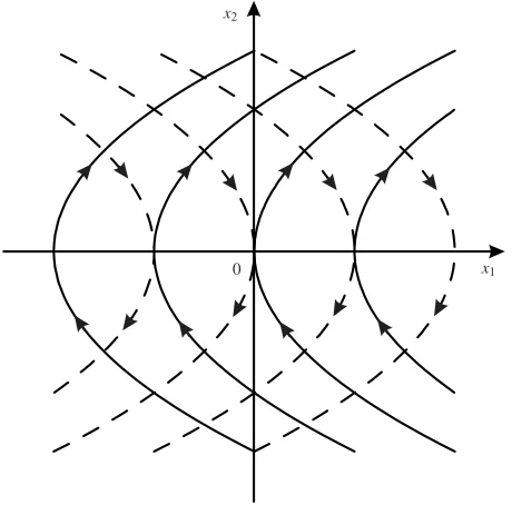
Let us consider arcs of phase trajectories in the(x1,x2)-plane corresponding to
u=1 andu=−1. By substitutingu=1 into (1.4.2), we obtain
dx1
dx2
=x2.
Integrating this equation, we get
x1=
1 2x
2
2+A, (1.4.10)
whereAis an arbitrary constant. Similarly, for the controlu=−1, we obtain from (1.4.2)
x1=−
1 2x
2
2+B, (1.4.11)
whereBis an arbitrary constant.
The families of parabolas corresponding to (1.4.10) and (1.4.11) are shown in

![Table 2.5 Variant 2: initial (q0i , ˙q0i ) and terminal (q∗i ) conditions, domain of possible motions([q−i ,q+i ]), control parameter (Xi), estimated (τ∗i ) and real(τi) motion times for the ith subsystem](https://thumb-ap.123doks.com/thumbv2/123dok/1324765.2012026/109.439.63.378.168.483/variant-initial-terminal-conditions-possible-parameter-estimated-subsystem.webp)
![Table 2.6 Variant 3: initial (q0i , ˙q0i ) and terminal (q∗i ) conditions, domain of possible motions([q−i ,q+i ]), control parameter (Xi), estimated (τ∗i ) and real(τi) motion times for the ith subsystem](https://thumb-ap.123doks.com/thumbv2/123dok/1324765.2012026/110.439.64.377.166.484/variant-initial-terminal-conditions-possible-parameter-estimated-subsystem.webp)
![Table 2.7 Variant 4: initial (q0i , ˙q0i ) and terminal (q∗i ) conditions, domain of possible motions([q−i ,q+i ]), control parameter (Xi), estimated (τ∗i ) and real(τi) motion times for the ith subsystem](https://thumb-ap.123doks.com/thumbv2/123dok/1324765.2012026/111.439.62.376.166.483/variant-initial-terminal-conditions-possible-parameter-estimated-subsystem.webp)