Full Terms & Conditions of access and use can be found at
http://www.tandfonline.com/action/journalInformation?journalCode=ubes20 Download by: [Universitas Maritim Raja Ali Haji], [UNIVERSITAS MARITIM RAJA ALI HAJI
TANJUNGPINANG, KEPULAUAN RIAU] Date: 11 January 2016, At: 20:47
Journal of Business & Economic Statistics
ISSN: 0735-0015 (Print) 1537-2707 (Online) Journal homepage: http://www.tandfonline.com/loi/ubes20
Modeling Conditional Covariances With Economic
Information Instruments
H. J. Turtle & Kainan Wang
To cite this article: H. J. Turtle & Kainan Wang (2014) Modeling Conditional Covariances With Economic Information Instruments, Journal of Business & Economic Statistics, 32:2, 217-236, DOI: 10.1080/07350015.2013.859078
To link to this article: http://dx.doi.org/10.1080/07350015.2013.859078
Accepted author version posted online: 13 Nov 2013.
Submit your article to this journal
Article views: 202
View related articles
Supplementary materials for this article are available online. Please go tohttp://tandfonline.com/r/JBES
Modeling Conditional Covariances With
Economic Information Instruments
H. J. T
URTLEDepartment of Finance, College of Business & Economics, West Virginia University, P.O. Box 6025, Morgantown, WV 26505 ([email protected])
Kainan W
ANGDepartment of Finance, College of Business and Innovation, University of Toledo, Mail Stop 103, Toledo, OH 43606 ([email protected])
We propose a new model for conditional covariances based on predetermined idiosyncratic shocks as well as macroeconomic andowninformation instruments. The specification ensures positive definiteness by construction, is unique within the class of linear functions for our covariance decomposition, and yields a simple yet rich model of covariances. We introduce a property,invariance to variate order, that assures estimation is not impacted by a simple reordering of the variates in the system. Simulation results using realized covariances show smaller mean absolute errors (MAE) and root mean square errors (RMSE) for every element of the covariance matrix relative to a comparably specified BEKK model with
owninformation instruments. We also find a smaller mean absolute percentage error (MAPE) and root mean square percentage error (RMSPE) for the entire covariance matrix. Supplementary materials for practitioners as well as all Matlab code used in the article are available online.
KEY WORDS: Covariance decomposition;Owninformation variables.
1. INTRODUCTION
Modeling the second moments of financial asset returns has important implications in risk management, derivative pricing, hedging, and portfolio optimization. A vast literature related to the time-varying covariance structure of asset returns has de-veloped from the seminal work of Engle (1982) and the subse-quent GARCH extension by Bollerslev (1986). Two illustrative examples of such work are Bollerslev, Engle, and Wooldridge (1988) and Turtle, Buse, and Korkie (1994). A variety of eco-nomic models also examine multivariate relationships between first and second moments. Continued improvement in covari-ance estimation will provide important benefits in the area of financial economics.
Developments in the estimation of multivariate second mo-ments include, among others, the constant conditional correla-tion (CCC) model of Bollerslev (1990); the factor ARCH model of Engle, Ng, and Rothschild (1990); the BEKK model of Baba et al. (1991) and Engle and Kroner (1995); the dynamic condi-tional correlation (DCC) model of Engle (2002) or the related model of Tse and Tsui (2002); and the spline-GARCH model of Rangel and Engle (2012). These models provide varying degrees of success in capturing the volatility clustering, leptokurtosis, and asymmetry commonly observed in economic and financial time series.
Two important challenges exist when modeling second mo-ments. First, positive definiteness of the covariance matrix must be ensured without spuriously imposing or restricting temporal patterns in conditional covariances. Second, important known economic information instruments must be allowed to impact the resultant covariances.
To address the positive definiteness issue, numerous ap-proaches have been proposed. For instance, the popular BEKK model ensures positive definiteness by writing the covariance
matrix as the sum of multiple positive definite matrices. In the DCC framework, restrictions on correlation parameters are im-posed in a multistep procedure that facilitates large-scale es-timation. A well-known drawback with these approaches is that the model structure may inadvertently impact the under-lying economic dynamics describing the evolution of second moments. Engle and Kroner (1995) explicitly recognized this potential undesirable impact when only one lag is included. They further provided necessary conditions for a general BEKK model with additional lags to achieve full generality. One ben-efit of our model is that we do not impose implicit restrictions within the class of linear specifications that we consider for our decomposition.
With regard to information instruments, we differentiate be-tween two sources that affect covariances—aggregate informa-tion that impacts all covariances, andowninformation that may be specific to particular asset return covariances. Schwert (1989) provided an early examination of how aggregate information might be expected to impact asset return volatilities for a va-riety of sources including trading days, lagged market trading volume, lagged market leverage, recession indicators, and ag-gregate financial leverage, among others. Later work by Glosten, Jagannathan, and Runkle (1993) shows that Treasury bill rates impact equity return variances. In addition to aggregate infor-mation effects, our model allowsowninformation for a given asset return to impact both the variance of that portfolio and also the covariance of that portfolio with other portfolios.Own
effects will vary across different assets in many economic con-texts. For example, firm-specific leverage decisions give rise
© 2014American Statistical Association Journal of Business & Economic Statistics April 2014, Vol. 32, No. 2
DOI:10.1080/07350015.2013.859078
217
to increases in both systematic and unsystematic risk that may not be captured in aggregate measures. Unfortunately, general specifications that allow information on any asset to impact any other asset suffer from a curse of dimensionality in large systems without further structure.
In many financial economic contexts, we are primarily in-terested in the role of owneffects with little impact expected from other assets in the system. Thus, in our study we examine a class of specifications in which the covariance between assets
iandjis impacted byowninformation related only to these two assets, and not any other assetk. Our model is parsimonious and feasible to estimate in settings withownimpacts for 10, or more assets. The proposed approach is practical for most asset allocation and performance evaluation studies as well as many empirical, portfolio-based investigations.
In this article, we consider linear specifications within a co-variance decomposition. We introduce a property, invariance to variate order, that assures estimation is not impacted by a simple reordering of the variates in the system. This simple ap-proach yields a unique result for covariances. Intuitively, we allow known information relatedonlyto asseti, say Zi,t−1, to
impact theith row of our (lower triangular) covariance decompo-sition, for all columns. This provides a large reduction in model parameters, and a rich model structure that includes informa-tion instruments forbothassetsiandjin covariances between assetsiandj. The resulting covariances from our model include a constant as well as terms inZi,t−1,Zj,t−1, andZi,t−1Zj,t−1.
Our invariance to variate orderproperty provides a valuable structure for the development of our model and produces a rich and parsimonious functional form not available in the extant literature.
Our approach will benefit many studies that examine how
owneconomic, financial, or fundamental accounting variables may impact expected returns, and potentially conditional co-variances. The literature in this area is extensive. For example, returns that are anomalous relative to the CAPM have been found for small capitalization companies (Banz1981), and value com-panies with large book-to-market equity (Rosenberg, Reid, and Lanstein1985). In addition, Fama and French (2008) provided a summary of how these types of anomalous returns may arise in models related to stock issuance, accruals, and momentum.
The extensive literature examining howownexogenous vari-ables may impact conditional variances suggests that a related investigation of covariances is worthy of pursuit. For example, Lamoureux and Lastrapes (1990) demonstrated thatownvolume has a highly significant impact on variance. Hagiwara and Herce (1999) considered howowndifferences from U.S. interest rates impact currency variances. Engle and Patton (2001, sec 2.3) discussed how non-GARCH-type variables, including macroe-conomic announcements and calendar-based regularities, may provide information to describe conditional variances. Although there is extensive research that examines how these and other fundamental portfolio characteristics may impact portfolio ex-pected returns, there is little work that studies how these same
own portfolio economic characteristics might impact covari-ances, and ultimately portfolio risks across a broad multivariate time series. In fact, beyond the highly successful BEKK ap-proach, there is little accepted practice to model covariances in multivariate settings. As demonstrated in our simulations, our
model is well behaved by standard measures of statistical per-formance and in comparison to the BEKK design. Further, the impact ofowninformation effects on conditional second mo-ments can be readily implemented without a large increase in model parameters.
The essence of our approach results from two observations. First, any positive definite matrix can be written as a lower tri-angular matrix multiplied by its transpose. Second, a simple reshuffling of asset returns should not produce a different func-tional form for the resultant covariance terms. Our strategy is to consider the class of models such that eachi,jelement of the covariance matrixdecompositionis linear in the underlying
owninformation instruments,Zi,t−1andZj,t−1. Linearity in this
decomposition can be motivated with a Taylor approximation using well-chosen instruments, even for potentially complex nonlinear underlying specifications. The general principles of our development can be readily extended to include higher or-der quadratic or cubic terms, at a cost of additional parameters. We recognize that our proposed methodology will give rise to a relatively large number of parameters in its most general form. However, our approach does offer improvement over currently available options. As is well known, estimation of even sim-ple unconditional samsim-ple covariance matrices is difficult when the number of assets is large, and the problem worsens as the number of assets increases relative to the number of time series observations (Jobson and Korkie1980). As a recent example, DeMiguel, Garlappi, and Uppal (2009) claimed that over 3000 monthly observations (250 years of data) would be needed to implement optimal portfolio choices in a context with 25 un-derlying assets. A number of approaches have been proposed to mitigate some of these estimation problems. A good represen-tative Bayesian covariance example is provided by Ledoit and Wolf (2004a,2004b) who shrunk the sample covariance matrix to a target value.
When modeling covariances acrossNassets, there areN(N2−1) unique covariance terms at each point in time. Because our in-terest is in parameterizing each unique term in a covariance matrix, the set of parameters quickly becomes large asN in-creases. Relative to existing alternatives that admitowneffects, our covariance modeling approach substantially mitigates this “curse of dimensionality.” In particular, our proposed method requires only oneowneffect regressor in each unique covariance decomposition term. This yields well-specified covariances in a parsimonious manner. For example, when examined relative to a comparably specified BEKK model, our approach requires 40% fewer parameters in a system of 10 variates. As we discuss in Section 2, our model can be further specialized to reduce parameters, at a cost of some generality.
Although the proposed model gives rise to a large number of parameters when the asset space is large, our approach is applicable in many common financial contexts. Because finan-cial decisions may often be simplified to consider a small set of well-diversified portfolios rather than the thousands of under-lying individual securities, our model is of value in most asset pricing studies and asset allocation decisions. For example, aca-demic financial literature often examines subsets of assets to replicate the important choices faced by investors. These asset subsets may be denoted asspanningorintersectingportfolios (Huberman and Kandel 1987). From a practical perspective,
Brinson, Hood, and Beebower (1986) found that a small num-ber of asset class portfolios explain a significant component of overall portfolio performance. They inferred that financial plan-ning and pension investment may be best achieved with only a small set of index funds.
Our conditional covariance model is intended to provide an economic description of second moments as a function of known economic information instruments, rather than as a time series motivated specification. This approach has the potential to be employed within an asset pricing investigation that provides nonlinear relations between economic variates and required as-set returns. Typical asas-set pricing tests are examined in the con-text of return portfolios that reduce the asset dimensionality to 2, 5, or 10. In these sorts of research designs, our estimation approach will have little difficulty for longitudinal samples of 10 years or more, as is common in application. Although our interest is largely related to economically motivated and known information instruments, our specification may also be readily adapted to a purely time series context as demonstrated in our empirical analysis.
In empirical simulations, we compare our model to a famil-iar multivariate ARCH specification for the covariance matrix suggested by the BEKK model. By construction, our linear in-formation instrument model has the potential to capture nonlin-ear economic relationships between variates that may be missed in existing specifications. Our design outperforms the BEKK alternative for all terms in the resultant conditional covariance matrix when measured by mean absolute errors (MAE) and root mean square errors (RMSE). When using heteroscedasticity-adjusted mean squared errors (HMSE), we find that for all but one covariance term, our model has greater estimation accu-racy than a comparable BEKK specification. In addition, our model contains fewer parameters than the BEKK design. Our simulation experiments also confirm that the proposed model outperforms the BEKK specification for all multivariate metrics of performance.
The research design proposed in this article may be readily nested within any well-specified model for conditional means. In particular, our approach has the potential to link an econom-ically motivated description of expected asset returns (through conditional mean specifications) within the context of a model describing evolving risks (through covariances). Although we focus on predetermined economic information instruments, a variety of parametric and nonparametric alternatives to model both means and covariances can also be considered. Fan and Yao (2003) provided a complete treatment of potential time series approaches available to examine conditional moments.
Covariance estimation may also be based on an underlying model of conditional means with a defined small set of common risk factors. These factor-based approaches effectively reduce the dimensionality of the asset portfolio covariance matrix by linking asset conditional means and covariances to underlying factor sensitivities. Examples of work in this area include Fan, Fan, and Lv (2008), who considered a defined set of risk factors for all assets, or Gagliardini, Ossola, and Scaillet (2011), and Fan, Liao, and Mincheva (2011), who employed factor model and sparse matrix techniques. Our work relates directly to this area of study. Intuitively, our focus is on how a moderate num-ber of portfolio returns behave in relation to known underlying
economic information instruments. Restricted versions of our model may extend our approach to consider larger asset sets without an excessive number of parameters, in a manner akin to factor-based models (see, e.g., the Appendix Bdevelopment). Our general model may also be used to describe the covariance dynamics within the mimicking factor portfolios from these works in order to examine how factor return moments are re-lated to known economic information instruments.
In addition, our approach can be compared to the extant lit-erature that uses Cholesky decompositions in a longitudinal context. Much of this research examines the interesting cross-correlations of disturbances over time. For example, Pinheiro and Bates (1996) provided an excellent discussion of five po-tential strategies to ensure positive definiteness in the estimation of covariance matrices that also allows estimation to proceed in an unconstrained manner. They favored Cholesky-type decom-positions to best estimate covariance behavior, with a prefer-ence for a spherical representation of decomposition elements. Pourahmadi (1999, 2000) used Cholesky decompositions to specify intertemporal covariances (or their inverses) between period tandt-jdisturbances for j=0, 1, 2,. . .,t-1. Pourah-madi’s work is similar in spirit to the approach in Gallant (1987) who used a Cholesky decomposition to model the inverse of a re-lated covariance matrix when fitting autocovariances in whole-sale prices (chap. 2, example 1). In our study, we focus on covariances across assets at a point in time, and how these covariances may change over time. Further, we are particu-larly interested in specifications that admit the impact of known
own economic variables while ensuring positive definiteness. Thus, our research dovetails with the longitudinal literature and suggests interesting avenues for future studies as these fields converge.
The remainder of the article is organized as follows. Sec-tion2presents our model specification, discusses the resultant positive definiteness of the covariance matrix, and describes theinvariance to variate orderproperty. We also examine our specification relative to a comparable version of the BEKK de-sign. Section3presents the empirical performance of our model in a large sample simulation. To confirm that our findings are not dependent on a large time series sample, we also present supportive finite sample simulation results and robustness tests. Concluding remarks are provided in Section4.
2. MODEL DEVELOPMENT
We begin with an intuitive presentation of our approach in a simple two-asset case. Consider a system comprised of a value portfolio, r1t, and a growth portfolio, r2t, both of which are potentially influenced by the known average research and de-velopment expenditures of the firms within these portfolios. We hypothesize that firms with greater research and development expenditures are more opaque and, hence, more risky (Baker and Wurgler2006). Other examples of importantowneconomic in-formation instruments abound and include financial statement information, previous price to earnings ratios, liquidity mea-sures, leverage meamea-sures, dividend yields, or any other charac-teristics that vary in the cross-section and over time.
To focus on covariance estimation, let rt=[r1t r2t] be a zero mean vector with conditional covariance matrix, Mt=[m11t m12t
m21t m22t]. Our primary interest is to provide an empiri-cal specification for covariances related to underlyingown port-folio research and development expenditures. Let the known economic information instruments be the average research and development expenditures for each portfolio, which we denote byZt−1=[Zi,t−1] fori=1 and 2. That is, we have a particular
interest in the research and development expenditures specific to each portfolio and not in the aggregate level of research and development expenditure in the overall economy. We observe that every positive definite covariance matrix can be written as Mt=LtL′t, whereLtis a lower triangular matrix. We consider a specification for each element in Lt =[lij t] that is linear in Zt−1, and examine a simple form forlij t,
lij t =γij0+γij1Zi,t−1 (1)
for i≥j, j =1, and 2; and model parametersγij0 andγij1.
Direct multiplication yields the resultant covariance matrix as
Mt =
Evaluating term by term, we see that m11t is a linear func-tion of Z1,t−1 andZ12,t−1; m22t is a linear function of Z2,t−1
andZ2
2,t−1; andm12t is a linear function ofZ1,t−1,Z2,t−1, and
Z1,t−1Z2,t−1. That is, the resultant variances,miit, are impacted by the own portfolio research and development expenditure,
Zi,t−1, as well as its square,Zi,t2−1, and covariances are impacted
by research and development expenditures for both portfolios in the system, throughZ1,t−1,Z2,t−1, andZ1,t−1Z2,t−1.
The model has some important features. First, the functional form of each element in Mt with respect to the information instruments is easily interpreted. For example, the variance of each portfolio’s return depends only on the firm-specific mation, where the covariance is driven by the economic infor-mation for both portfolios. Second, the model ensures positive definiteness ofMtif each diagonal element inLtis nonzero (see AppendixA). Third, the specification given by Equation (1) is theuniquelinear function ofowninformation instruments that ensures covariances are not spuriously modified by a simple reordering of the portfolios in the system. We call this final propertyinvariance to variate order.
Definition: A model is said to satisfy the condition of in-variance to variate orderif the functional form for all variance and covariance specifications includes the same independent information instruments when the variate order is perturbed.
To understand the importance of the invariance to variate orderproperty, note that Equation (1) satisfies the condition that variate order will not impact the functional form of covariances.
If we were to estimate the trivially reordered system,
r∗t =
the functional form for the two variates would not change. We view this property as desirable and only consider models that satisfy this condition. In our empirical application, this condition ensures that each pair from our five portfolio return series has the same functional form for each potential covariance specification. Surprisingly, many intuitive linear specifications forlij t do not pass the test ofinvariance to variate order. For example, consider the more exhaustive specification,
lij t =
This specification admits terms in bothZi,t−1andZj,t−1for all
lij t terms. Direct multiplication yields the resultant covariance matrix as
Evaluating term by term, we observe that m11t is a linear function ofZ1,t−1 andZ12,t−1, where m22t is a linear function ofZ1,t−1,Z2,t−1,Z1,t−1Z2,t−1,Z21,t−1, andZ
2
2,t−1. If the order
of the two assets were changed, the functional form for the two variates would change due solelyto variate order. Therefore, specification (3) does not satisfy theinvariance to variate order
property.
2.1 Model
Our goal is to provide an economically driven specification for time varying covariances that is parsimonious, yet rich in de-scribing covariances as a function of the underlying economic state. To focus solely on covariance estimation, consider an
N×1 zero mean random vector, rt, with associated condi-tional covariance matrix, Mt≡Et−1[rtr′t], for t =1, . . . , T. We wish to consider potential specifications forMt related to underlying economic information instruments that may be ei-ther lagged endogenous variables, or any oei-ther known observ-able economic information instruments from the information set. For clarity, we consider two general types of economic in-formation instruments,owneconomic information instruments,
Zi,t−1,i=1, . . . , Nthat are specific to each series considered,
as well as aK×1 vector of macroeconomic sources of infor-mation,Zagg,t−1. In equilibrium, we might consider the relation between covariances of abnormal asset returns to both individual asset characteristics as well as observed market characteristics.
For example, stock or portfolio covariances may be dependent onownfinancial characteristics such as liquidity, opaqueness, profitability, or valuation measures like price-to-book or cash-flow-to-book. In addition, overall market forces such as general credit conditions might impact conditional covariances.
Our general framework considers the time varying condi-tional covariance matrix, Mt =[mij t], for i, j=1,2, . . . , N, and fort =1, . . . , T. For each conditional covariance matrix, Mt, we consider the following decomposition,
Mt=Lt(θ|t−1)Lt(θ|t−1)′, (5)
where θ represents a vector of parameters, t−1 represents a
vector of information instruments, andLt(θ|t−1) is any lower
triangular matrix with nonzero diagonals.Ltis not a Cholesky decomposition of Mt, as we do not require strictly positive diagonal entries inLt.
Our interest is in a particular form for the nonzero elements within Lt(θ|t−1)=[lij t(θ|t−1)] from the general class of
linear functions in aggregate information instruments, and in
owninformation instruments defined as
lij t(θ|t−1)=
⎧ ⎨ ⎩
γii0+γ′ii1Zagg,t−1+γii2Zi,t−1, fori=j
γij0+γ′ij1Zagg,t−1+γij2Zi,t−1 fori > j
+γij3Zj,t−1,
(6)
wherei, j=1,2, . . . , N,i≥j; Zagg,t−1 is aK×1 vector of macroeconomic sources of information; Zi,t−1 andZj,t−1 are
known own information instruments for the ith and jth vari-ate, respectively; and whereγij0,γij1,γij2, andγij3are known
conformable parameters. For all i < j =1,2, . . . , N we set
lij t =0.
To simplify our notation, we write the class of linear functions as
lij t(θ|t−1)=θZ, (7)
where θ=[γij0,γ′ij1, γij2] and Z=[1,Z′agg,t−1, Zi,t−1]′ for
i=j; and θ=[γij0,γ′ij1, γij2, γij3] and Z=[1,Z′agg,t−1,
Zi,t−1, Zj,t−1]′fori > j.
Proposition 1: Within the general class of functions defined by Equation (6), for some predetermined variablesZagg,t−1and
Zi,t−1, the functional form given by
lij t(θ|t−1)=γij0+γ′ij1Zagg,t−1+γij2Zi,t−1 (8)
ensures a unique covariance specification, ensures positive def-initeness for the resultant covariance matrixMt provided that the coefficients γii0 are nonzero for all i=1,2, . . . , N, and
satisfies theinvariance to variate orderproperty.
Proof: See AppendixA.
Our proposed specification is similar in spirit to a Cholesky decomposition of the conditional covariance matrix. This de-composition is often used in constant covariance applications where positive definiteness is required, and is found in the works of Pinheiro and Bates (1996) and Pourahmadi (1999, 2000) among others. Because every positive definite matrix
yields a unique Cholesky decomposition, we build our speci-fication for second moments within the lower triangular matrix context. Following Pinheiro and Bates (1996), we ignore the degenerate case of a positive semidefinite covariance matrix, and focus solely on the positive definite case. Given our con-cern that uniqueness is solely related to the resultant covariance specification and not to the decomposition, Lt, we do not im-pose the Cholesky condition that diagonal elements must be strictly positive. Rather, these elements must only be nonzero. An interesting alternative form provided by Pinheiro and Bates (1996) models the log of the diagonal elements ofLtto ensure positivity in an unrestricted manner and uniqueness in the de-composition. Untabulated estimation results, which impose the additional condition that diagonal elements of the lower trian-gular matrixLt are positive for all times and variates, produce very similar results.
The number of parameters required to estimate our proposed system offers an improvement over existing models. In general, each of the N(N2+1) uniquelij t terms requires a specification in our context. In the case of Equation (8) with a scalarZagg,t−1,
this results in3N(N2+1)total covariance parameters. For example, in a typical financial market application with 10 portfolios and 40 years of data, estimation of the 165 required covariance parameters is readily implementable, even with only monthly observations (480 time series observations).
In Appendix A we provide sufficient conditions to ensure the asymptotic consistency and normality of maximum like-lihood estimates and discuss some recent literature providing more general related results. Further research to estimate mod-els of this sort with semiparametric techniques (Engle and Gonzalez-Rivera 1991), estimating functions (Li and Turtle 2000), or nonparametric approaches (Wu and Pourahmadi2003 or Yao and Li2013) may also be worthwhile.
2.2 Comparisons With a BEKK-Like Covariance Model
Although our interest is primarily in economically motivated changes in second moment matrices, our approach can be com-pared to the extant time series literature by specifying our in-formation instruments as time series variables. In particular, we compare the multivariate ARCH representation of the BEKK model to a restricted version of Equation (8) with no macroeco-nomic information instruments,
lij t(θ|t−1)=γij0+γij1Zi,t−1. (9)
We define the following covariance specifications for the lin-ear information instrument and BEKK models,
Mt=LtL′t =[mij t], (10)
and
MBEKKt=C0C′0+A1rt−1r′t
−1A′1, (11)
respectively, where C0and A1 areN×N parameter matrices and where C0 is lower triangular. Notice that to estimate the BEKK covariance matrix, MBEKKt, we require N(N+1)
2 +N 2
parameters given there are N(N2+1) parameters in C0 andN2
parameters in A1.
To facilitate comparison with our linear information instru-ment model, we replacert−1withZt−1for the BEKK specifica-tion in Equaspecifica-tion (11). Therefore, in the simplest bivariate case, Mtis given byMt =[m11t m12t
The related BEKK representation is given by
MBEKKt =
A comparison of Equations (12) and (13) reveals four im-portant findings: (1) Both models satisfy theinvariance to vari-ate order property. (2) Our model given by Equation (9) is more parsimonious than the BEKK-like model. In particular, for anyN×N covariance matrix, Mt hasN(N+1) parameters, whereMBEKKtrequiresN(N+1)
2 +N
2parameters. Thus, for any
N ≥2, N(N2+1)+N2> N(N+1). For example, in a system of 10 variates, the BEKK model will require an increase of 40% (=(155–110)/110) in required parameters. (3) Our covariance matrix,Mt, is the unique representation given the general class of models described in Equation (6). (4) Our conditional covari-ance matrix has a distinctly different functional form relative to BEKK. Specifically, eachi, jth element of the BEKK covariance matrix is a function ofZ2
i,t−1,Zj,t2 −1, andZi,t−1Zj,t−1. In
con-trast, our approach yields a covariance matrix where variances are solely functions of own instruments, and covariances be-tweeniandj are functions ofZi,t−1,Zj,t−1, andZi,t−1Zj,t−1.
Our approach, therefore, has the ability to capture interesting
own effects involving lower moments of the instruments that may be obscured within the BEKK functional form.
Much of the extant literature asserts that the BEKK and DCC models often perform similarly in forecasting conditional co-variances. For example, Caporin and McAleer (2008) found that
the scalar versions of the two models are similar in forecasting conditional covariances and value-at-risk thresholds. Further, Massimiliano and Michael (2010) suggested that the BEKK and DCC (or CCC) models produce highly comparable condi-tional covariances and correlations in both univariate and large scale contexts. Given these findings, and our primary interest inowneffects, we focus our empirical analysis on a detailed comparison of our linear information instrument model and the BEKK model.
Conceptually, however, a similar special case of our model can be compared to other models such as the factor ARCH model of Engle, Ng, and Rothschild (1990), using a restricted version of Equation (8) with only macroeconomic information instruments, such as,lij t(θ|t−1)=γij0+γ′i1Zagg,t−1. In
Ap-pendixBwe discuss the similarities between this specialized form of our model and the factor ARCH. Methodologically, this restricted approach has similarities with Fan, Fan, and Lv (2008), Gagliardini, Ossola, and Scaillet (2011), and Fan, Liao, and Mincheva (2011) who considered a small set of contempo-raneous risk factors to describe conditional asset return means. The most general representation of the multivariate ARCH model is the unrestricted vech form Bollerslev, Engle, and Wooldridge (1988), which for the multivariate ARCH(1) model yields,mt =ω+A1ηt−1, wheremt=vech(Mt),ηt =
vech(rtr′
t) and vech is the matrix operator that stacks the lower triangular part of a symmetricN×NmatrixMtinto anN(N+1)
2
dimensional vector, and whereωandA1are parameter matrices with dimensions N(N2+1)×1 and N(N2+1)×N(N2+1), respec-tively. Although general, the vech representation is not practical to implement without additional restrictions to ensure covari-ance matrix positive definiteness.
3. EMPIRICAL ANALYSIS
We present empirical results for covariance matrix estimation using our linear information instrument model and a comparable specification of the BEKK model. Our empirical results focus on a comparison of the underlying choice parameters in Equations (10) and (11). In many empirical applications a restricted form of MBEKKt is considered in which the parameter matrixA1 is diagonal, orA1is equal to a scalar parameter times the identity matrix. For brevity, we avoid a comparison of restricted versions of the BEKK model and similarly restricted versions of our linear information instrument model.
Our empirical analysis is comprised of three general sections. Initially, we establish that the proposed approach behaves well in a lengthy time series in comparison with the BEKK specifi-cation. Then, we demonstrate that the linear information instru-ment model has desirable finite sample properties for various time series sample sizes and asset dimensions. Finally, we offer results that demonstrate our findings are robust to alternative co-variance specifications, information instrument definitions, and asset sets.
Our primary empirical applications make use of a lengthy sample of realized conditional covariance matrices for five book-to-market (BM) portfolios that we treat as the true value to be estimated using the two competing procedures. Our methodol-ogy can also be applied to a number of other owneconomic
or financial variables of interest in asset allocation and per-formance evaluation studies, or portfolio-based asset pricing investigations.
3.1 Conditional Covariance Matrix Construction
We construct weekly conditional covariance matrices from daily returns of the value-weighted book-to-market (BM) quintile portfolios over the period July 5, 1963, to Decem-ber 30, 2009. Our sample begins on Friday, July 5, be-cause Thursday, July 4, was a market closure for the Inde-pendence Day holiday. Portfolio return data are downloaded from Ken French’s website: http://mba.tuck.dartmouth.edu/ pages/faculty/ken.french/data library.html.
To avoid spurious weekend and holiday effects, we define a week from Thursday-open to Wednesday-close. By choosing this weekly period, we mitigate the impact of market closures and provide the greatest number of possible five-day trading weeks. Because our analysis is focused at the portfolio level, missing observations reflect U.S. market closures. Our sample contains 2419 Thursday to Wednesday calendar weeks of which 2413 have either four (413) or five (2000) trading days per week. The worst period for available data was from Thursday, July 4 to Wednesday, July 10, 1968. The market was closed on July 4 (Independence Day), July 5 (the day after Independence Day), July 6 and 7 (the weekend), and July 10 (the 1968 Paperwork crisis). This produced a two-day trading week that included only Monday, July 8 and Tuesday, July 9. These closures also resulted in a related four-day trading week that followed.
Weekly realized conditional covariance matrices are con-structed as follows. For each Wednesday ending on dayt, we compute the weekly realized covariance matrices using daily re-turns for the current and previous seven weeks of daily rere-turns as
covt=5× 1
Ndays
Ndays
j=1
rd,T+1−jrd,T′ +1−j (14)
whererd,T+1−j is the vector of percentage daily returns on trad-ing dayT +1−j,T is the last trading day in the week under consideration, andNdaysis the number of trading days in the
cur-rent and previous seven weeks (for a total 8-week window used to construct realized covariances). Thus, similar to Andersen et al. (2001) and the empirical mixed data sampling (MIDAS) results from Ghysels, Santa-Clara, and Valkanov (2006), we cre-ate weekly realized conditional covariance matrices by scaling each daily realized covariance matrix by five to create a weekly measure.
We treat this calculated time series of realized covariance matrices as the population values to be subsequently estimated using either our linear information instrument model or the BEKK model. At each point of time,t, we draw a weekly return vector rt from a multivariate normal distribution with mean of zero and covariance matrix of covt as in Equation (14). This procedure creates a lengthy multivariate time series ofT=2419 weekly observations for the BM quintile portfolios (N=5) that we treat as our base case sample for later empirical simulations.
In robustness tests, we find our empirical results are compa-rable when using modified realized conditional covariance con-struction methods with different previous return windows and varied decay weights for lags of previous daily squared returns. Although the general magnitudes of the model performance met-rics change with covariance construction assumptions, the su-perior performance of the linear information instrument model relative to the BEKK model persists in all cases.
3.2 Conditional Covariance Matrix Estimation
The maximum likelihood (ML) estimator of the covariance matrix, T1 T
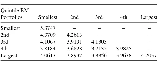
t=1(rt−r¯)(rt−r¯)′,for the 5×1 set of book-to-market simulated portfolio returns,rt, with sample mean ¯r, is reported for the weekly sample of 2419 simulated observations inTable 1. The simulated series is based on a normal draw with a 5 × 1 zero mean vector and a time-varying covariance matrix given by Equation (14).
To begin our empirical analysis, we report the estimated constant covariance matrix using our ML routine for the sim-ulated series. The general log-likelihood function is given by log(θ|rt)= −1
2
2419
t=1 [Nlog(2π)+log|Mt| +r′tM−
1
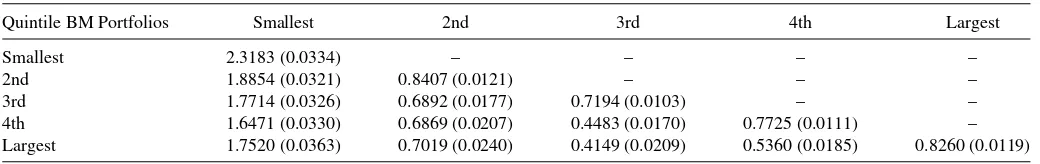
t rt], whereMtis the conditional covariance matrix att. For the case of a constant covariance matrix, we parameterize the lower trian-gular matrixL=[lij] as,lij =γijfori≥j, i, j =1,2, . . . ,5; and wherelij is thei,jth element ofL. The covariance matrix is then constructed as,M=L L′.Table 2reports the constant co-variance matrix in lower triangular form,L=[γij], along with associated standard errors in parentheses. Starting values for the mean vector are given by zeros and the initial value ofγij is the i, jth element of the Cholesky decomposition of the uncondi-tional sample covariance matrix. We use the quasi-Newton algo-rithm in Matlab with the Broyden–Fletcher–Goldfarb–Shanno (BFGS) formula for updating the Hessian.
We note that allγijterms are typically magnitudes larger than their standard errors. In addition, after multiplication, we find that the resultant estimated unconditional covariance matrix, M =L L′, is virtually identical to the ML estimate of the
co-variance matrix inTable 1. Although we follow the conventional practice of discussing individual tests in many tables, we rec-ognize that na¨ıve usage of multiple individual tests will tend to find too many significant variables. For example, with a test size of 5%, we recognize that one in 20 tests will incorrectly reject
Table 1. The estimated unconditional maximum likelihood (ML) covariance matrix
Quintile BM
Portfolios Smallest 2nd 3rd 4th Largest
Smallest 5.3747 – – – –
2nd 4.3709 4.2613 – – –
3rd 4.1067 3.9191 4.1303 – –
4th 3.8184 3.6828 3.7135 3.9825 –
Largest 4.0617 3.8932 3.8856 3.9678 4.7037
NOTE: The maximum likelihood estimator of the covariance matrix of simulated weekly returns for five book-to-market (BM) portfolios,rt, is given by1
T
T
t=1(rt−r¯)(rt−¯r)′
for theT=2419 observations, with sample mean vector, ¯r. The simulated series is based on a normal draw with zero mean and time-varying covariance given by Equation (14).
Table 2. Unconditional estimate of the covariance decomposition,L
Quintile BM Portfolios Smallest 2nd 3rd 4th Largest
Smallest 2.3183 (0.0334) – – – –
2nd 1.8854 (0.0321) 0.8407 (0.0121) – – –
3rd 1.7714 (0.0326) 0.6892 (0.0177) 0.7194 (0.0103) – –
4th 1.6471 (0.0330) 0.6869 (0.0207) 0.4483 (0.0170) 0.7725 (0.0111) –
Largest 1.7520 (0.0363) 0.7019 (0.0240) 0.4149 (0.0209) 0.5360 (0.0185) 0.8260 (0.0119)
NOTE: The ML estimate of the unconditional covariance matrix decomposition for simulated weekly returns. The unconditional ML estimate of the covariance matrixM=L L′, where
L=[lij] is a lower triangular matrix withi, jth elementlij=γij. We report ML parameter estimates ofγijalong with standard errors in parentheses.
a true null. In our later analysis comparing across models, we also report joint tests of all parameters, as well as information criteria to assess overall model performance. A discussion of these issues can be found in Romano and Wolf (2005), Romano, Shaikh, and Wolf (2008), and Frahm, Wickern, and Wiechers (2012).
For our conditional covariance estimation, we evaluate the linear information instrument model given by Equation (9) ver-sus the BEKK-like model after computation ofMtusing Equa-tion (11). To facilitate comparison across models, we replace rt−1in Equation (11) with the information instrument realized at weekt–1,Zt−1 =[Zi,t−1], whereZi,t−1is the average of the daily absolute returns over the 4-week calendar period beginning 1 week prior to weekt. Also, we multiply the resultant instru-ment by 500 to provide a similar scale in all coefficient estimates with no impact on the resultant covariance estimates. This mod-ified instrument results in an improvement of greater than 300% in the MAPE for both the linear instrument and BEKK models in comparison with a single lag of previous returns.
Initial values of the parameters for the linear information instrument model (from Equation (9)) are obtained using the current and previous 20 weeks of returns as follows. At each point in time t, we construct a square matrix in which thei, jth element isei,tej,t, whereei,t =211 k20=0(ri,t−k−r¯) and ¯ris the time-series average ofri,tover the entire sample period. We take the Cholesky decomposition of the square matrix [ei,tej,t] at each timet. For each element in the resultant lower triangular matrix after the decomposition, we run an ordinary least squares (OLS) regression onZi,t−1to obtain the starting parameter
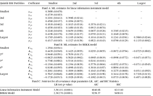
val-ues. To specify the BEKK model, we follow Equation (11) for MBEKKt, withrt−1=Zt−1. Initial values for the BEKK model (from Equation (11)) of the parameter matrixC0are obtained as the lower triangular matrix of the unconditional sample covari-ance matrix after Cholesky decomposition. The initial values of A1 are set to 0.05 for each element. Robustness checks with alternative starting values suggest the conditional covariance matrix estimates are not particularly sensitive to the choice of the initial value of A1. We also examined less precise starting values for the linear information instrument model to confirm that the superior empirical performance is not driven by starting parameter values. For both models, we follow Engle and Kroner (1995) and estimate parameters using the simplex algorithm for the initial 20 iterations, and then the quasi-Newton algorithm in Matlab with the BFGS formula to obtain final parameter esti-mates. Parameter estimates and standard errors are reported in Table 3.
Table 3reports results for the linear information instrument model in Panel A and for the BEKK Model in Panel B. In Panel A we observe that virtually all 30 coefficients are typically a magnitude larger than the reported standard errors with the sole exception being the reported estimate ofγ420. Panel B shows
that the full BEKK model has a considerably larger number of parameters (40 versus 30), and many of these coefficients are comparable in magnitude to the reported standard errors. Inter-estingly,allabove diagonal terms in the A1 coefficient matrix are not significant when considered individually. Similarly, the lower triangular portion of theA1coefficient matrix, and espe-cially the diagonal elements, are often individually significant. The initial column of Panel C inTable 3reports the likelihood ra-tio test statistic and associatedp-value for the test that all covari-ance slope parameters are jointly zero for each model. We find strong evidence that both models offer important improvements over a constant covariance specification. The Akaike infor-mation criterion (AIC) and the Bayesian inforinfor-mation criterion (BIC) statistics are reported in the final two columns of Panel C to compare models. According to either information criterion, the linear information model is superior to the BEKK model.
To provide an alternative evaluation of the parameter es-timates in Panel A of Table 3, Table 4 presents the co-efficient estimates and standard errors for the parameters of the conditional covariance matrix after expanding the Mt =LtL′
t linear information instrument specification. The i, jth element in Mt, mij t, may be rewritten as mij t =
φij0+φij1Zi,t−1+φij2Zj,t−1+φij3Zi,t−1Zj,t−1, whereφij0=
j
k=1γik0γj k0, φij1=2
j
k=1γik1γj k0, φij2=0, and φij3=
j
k=1γik1γj k1 when i=j; and φij0=
j
k=1γik0γj k0,φij1=
j
k=1γik1γj k0,φij2=jk=1γik0γj k1, andφij3=jk=1γik1γj k1
wheni=j. Although our choice parameters arise within the elements of the lower triangular decomposition,Lt, by the func-tional invariance property of ML, the coefficient estimates of all
φij terms are also ML.
The standard errors for these coefficient estimates are derived using the delta method. Let γ be a given vector of parame-ters for the decomposition matrixLt and leth(γ) be a vector of coefficients for the resultant covariance matrix, Mt. Then, the coefficient estimateh( ˆγ) follows an asymptotically normal distribution given by
√
T(h( ˆγ)−h(γ))∼aN(0,∇h(γ)′·· ∇h(γ)) (15) where T is the number of observations, is the covariance matrix of γ, and ∇h(γ) is the gradient function of h(γ).
Table 3. Conditional covariance matrix estimation
Quintile BM Portfolios Coefficient Smallest 2nd 3rd 4th Largest
Panel A: ML estimates for linear information instrument model
Smallest γ110 0.3866 (0.0476) – – – –
γ111 0.4739 (0.0163)
2nd γ2j0 0.2201 (0.0412) 0.3986 (0.0214) – – –
γ2j1 0.4580 (0.0157) 0.1094 (0.0072)
3rd γ3j0 0.1616 (0.0402) 0.1015 (0.0318) 0.3574 (0.0211) – –
γ3j1 0.4550 (0.0163) 0.1460 (0.0116) 0.0913 (0.0074)
4th γ4j0 0.2248 (0.0430) 0.0459 (0.0360) 0.0857 (0.0328) 0.3385 (0.0215) – γ4j1 0.4196 (0.0176) 0.1563 (0.0137) 0.0793 (0.0121) 0.1049 (0.0078)
Largest γ5j0 0.1785 (0.0495) 0.1105 (0.0454) 0.1014 (0.0415) 0.1241 (0.0381) 0.3680 (0.0244) γ5j1 0.4317 (0.0185) 0.1327 (0.0158) 0.0621 (0.0143) 0.0790 (0.0129) 0.1135 (0.0082)
Panel B: ML estimates for BEKK model
Smallest C0
11 1.2504 (0.0541) – – – –
A1
1j 0.4439 (0.0549) 0.1425 (0.0955) 0.0293 (0.0855) −0.0872 (0.0794) −0.0725 (0.0602)
2nd C
02j 0.9440 (0.0591) 0.7639 (0.0117) – – –
A1
2j −0.0825 (0.0506) 0.5820 (0.0902) 0.0905 (0.0819) −0.0998 (0.0772) −0.0471 (0.0571)
3rd C
03j 0.7786 (0.0602) 0.5318 (0.0161) 0.6181 (0.0101) – –
A1
3j −0.1304 (0.0499) 0.1394 (0.0839) 0.5778 (0.0804) −0.0552 (0.0751) −0.0711 (0.0545)
4th C
04j 0.8186 (0.0595) 0.4996 (0.0183) 0.3018 (0.0167) 0.6694 (0.0110) –
A1
4j −0.2081 (0.0494) 0.1609 (0.0869) 0.1043 (0.0786) 0.3275 (0.0800) 0.0511 (0.0563)
Largest C0
5j 0.7647 (0.0646) 0.4869 (0.0208) 0.2492 (0.0196) 0.3414 (0.0176) 0.7326 (0.0132)
A1
5j −0.1720 (0.0513) 0.1926 (0.0916) −0.1062 (0.0813) 0.0733 (0.0838) 0.4671 (0.0626)
Panel C: Joint test for all covariance slope parameters LR, AIC, and BIC Statistics
LR test (p-value) AIC BIC
Linear Information Instrument Model 3,581.01 (0.0001) 8040.06 8213.80
BEKK Model 2,382.70 (0.0001) 9258.37 9490.01
NOTE: ML estimates for the linear information instrument model and the BEKK model for simulated weekly returns. For the linear information instrument model, the conditional covariance matrix is computed asMt=LtL′
t, whereLt=[lij t] is the lower triangular matrix att, andlij t=γij0+γij1Zi,t−1, for parametersγij0andγij1, andZi,t−1is the instrument
variable realized att−1. For the BEKK model, the conditional covariance matrix is modeled asMBEKKt=C0C′
0+A1Zt−1Z′t−1A′1, whereC0andA1are parameter matrices withC0
being lower triangular andZt−1is the instrument vector realized att−1. Panels A and B report the ML estimates for the linear information instrument model and the BEKK model, respectively. In both models, the information instrumentZi,t−1is computed as the previous four-week mean of absolute returns beginning one week prior. The standard errors of the
ML estimates, obtained as the square root of the diagonal elements of the inverse of the Fisher information matrix, are reported in parentheses. Panel C reports the LR joint test that all covariance slope parameters are equal to zero (with associated p-value in parentheses) as well as the AIC and BIC statistics for each model.
Standard errors ofh( ˆγ) may be computed using∇h( ˆγ)′·ˆ ·
∇h( ˆγ), where ˆ is the estimated covariance matrix of ˆγ and is obtained as the inverse of the Fisher information matrix. Be-cause each element of Mt is a function of ˆγ and known in-formation instruments, in Appendix A we also use the delta method to compute the standard errors for each estimated con-ditional covariance term from Equation (9). This approach may be of particular interest to practitioners interested in inferences regarding the resultant covariance estimates.
Interpretation of the coefficients in the expanded model is simplified in that estimates relate to the covariance matrix di-rectly. For example, the coefficient estimate ofφ111is 0.3664 and
suggests that a unit increase in the instrument value,Z1,t−1will
give rise to a 0.3664 unit increase in the smallest BM portfolio variance. In addition to this effect, we find a nonlinear impact related toZ2
1,t−1. Interpreting this individual coefficient, theφ113
estimate of 0.2246 suggests that, after controlling for absolute previous errors, a one unit increase in the squared instrument gives rise to a 0.2246 unit increase in the smallest BM portfolio variance. In general, we observe that the reported coefficients are a magnitude larger than the underlying standard errors, sug-gesting strong sensitivities to all instruments. The estimates in Table 4ensure positive definiteness for all covariance matrices
at each point in time by construction and allow for a wide range of complicated potential functional relationships between the information instruments and the covariance matrix.
3.3 Conditional Covariance Matrix Estimation by Information Instrument Percentile
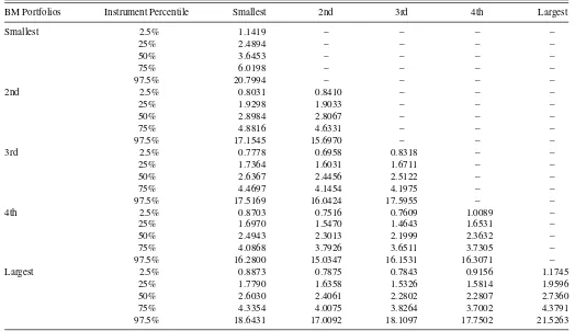
Table 5presents an alternative manner to gauge the economic importance of changes in the covariance matrix with underlying information instrument realizations. For each instrument we evaluate the impact of various percentile instrument realizations (including the 2.5, 25, 50, 75, and 97.5 percentiles) on estimated covariances. We then report the resultant conditional covariance matrix estimate for each percentile of instrument realizations using the parameter estimates fromTable 4.
Table 5shows that the variability in the estimated covariance matrix elements is economically important. In particular, all of the covariance estimates based on the 97.5 percentile instrument realizations are more than 15 times larger than the corresponding estimates based on the 2.5 percentile realization. Interestingly, we find more variability and a greater range in variances for the most extreme book to market portfolios, relative to the second, third, and fourth BM quartiles.
Table 4. Conditional covariance matrix coefficient estimates
Quintile BM Portfolios Coefficients Smallest 2nd 3rd 4th Largest
Smallest φ110 0.1494 (0.0368) – – – –
φ111 0.3664 (0.0349) – – – –
φ112 – – – – –
φ113 0.2246 (0.0155) – – – –
2nd φ2j0 0.0851 (0.0239) 0.2074 (0.0254) – – –
φ2j1 0.1770 (0.0191) 0.2888 (0.0324) – – –
φ2j2 0.1043 (0.0178) – – – –
φ2j3 0.2170 (0.0139) 0.2217 (0.0145) – – –
3rd φ3j0 0.0625 (0.0205) 0.0760 (0.0200) 0.1641 (0.0212) – –
φ3j1 0.1759 (0.0198) 0.1583 (0.0177) 0.2419 (0.0335) – –
φ3j2 0.0766 (0.0181) 0.0851 (0.0174) – – –
φ3j3 0.2156 (0.0136) 0.2243 (0.0139) 0.2367 (0.0153) – – 4th φ4j0 0.0869 (0.0233) 0.0678 (0.0221) 0.0716 (0.0197) 0.1746 (0.0245) – φ4j1 0.1622 (0.0186) 0.1547 (0.0169) 0.1120 (0.0168) 0.2876 (0.0317) – φ4j2 0.1065 (0.0194) 0.1080 (0.0186) 0.1168 (0.0187) – – φ4j3 0.1988 (0.0132) 0.2093 (0.0136) 0.2210 (0.0142) 0.2178 (0.0153) – Largest φ5j0 0.0690 (0.0237) 0.0834 (0.0213) 0.0763 (0.0213) 0.0959 (0.0213) 0.2052 (0.0297)
φ5j1 0.1669 (0.0194) 0.1479 (0.0178) 0.1054 (0.0176) 0.1352 (0.0178) 0.2992 (0.0382) φ5j2 0.0846 (0.0227) 0.0938 (0.0219) 0.1066 (0.0222) 0.1132 (0.0204) – φ5j3 0.2046 (0.0136) 0.2122 (0.0138) 0.2215 (0.0143) 0.2151 (0.0147) 0.2270 (0.0166)
NOTE: Conditional covariance matrix element-by-element coefficient estimates are given as a function of information instruments for the simulated weekly return sample. The conditional covariance matrix is estimated by the linear information instrument model defined aslij t=γij0+γij1Zi,t−1, wherelij tis thei,jth element in the lower triangular matrixLt. The covariance
matrix is then constructed asMt=LtL′t. Thei,jth element inMt, ismij t=φij0+φij1Zi,t−1+φij2Zj,t−1+φij3Zi,t−1Zj,t−1, whereφij0=jk=1γik0γj k0,φij1=2kj=1γik1γj k0, φij2=0, andφij3=kj=1γik1γj k1wheni=j; andφij0=jk=1γik0γj k0,φij1=jk=1γik1γj k0,φij2=jk=1γik0γj k1, andφij3=jk=1γik1γj k1wheni=j. The coefficients with
respect to the information instruments inmij tare functions of parametersγij0andγij1, and are estimated using ML. The table reports ML estimates of the coefficients with associated
standard errors given by the delta method in parentheses.
Table 5. Conditional covariance matrix estimates for percentiles of instruments
BM Portfolios Instrument Percentile Smallest 2nd 3rd 4th Largest
Smallest 2.5% 1.1419 – – – –
25% 2.4894 – – – –
50% 3.6453 – – – –
75% 6.0198 – – – –
97.5% 20.7994 – – – –
2nd 2.5% 0.8031 0.8410 – – –
25% 1.9298 1.9033 – – –
50% 2.8984 2.8067 – – –
75% 4.8816 4.6331 – – –
97.5% 17.1545 15.6970 – – –
3rd 2.5% 0.7778 0.6958 0.8318 – –
25% 1.7364 1.6031 1.6711 – –
50% 2.6367 2.4456 2.5122 – –
75% 4.4697 4.1454 4.1975 – –
97.5% 17.5169 16.0424 17.5955 – –
4th 2.5% 0.8703 0.7516 0.7609 1.0089 –
25% 1.6970 1.5470 1.4643 1.6531 –
50% 2.4943 2.3013 2.1999 2.3632 –
75% 4.0868 3.7926 3.6511 3.7305 –
97.5% 16.2800 15.0347 16.1531 16.3071 –
Largest 2.5% 0.8873 0.7875 0.7843 0.9156 1.1745
25% 1.7790 1.6358 1.5326 1.5814 1.9596
50% 2.6030 2.4061 2.2802 2.2807 2.7360
75% 4.3354 4.0075 3.8264 3.7002 4.3791
97.5% 18.6431 17.0092 18.1097 17.7502 21.5263
NOTE: The conditional covariance matrix estimates for the 2.5, 25, 50, 75, and 97.5 percentiles of the information instruments for the simulated weekly return sample. Percentile values are computed for each information instrument across the entire sample period for all five portfolios. ML conditional covariance matrix estimates are computed using the coefficients described inTable 4.
Table 6. Comparing the estimation accuracy of the linear information instrument and BEKK covariance models
Quintile BM Portfolios Smallest 2nd 3rd 4th Largest
Panel A: MAE Linear Inst. Model [BEKK Model]
Smallest 1.3668∗∗∗[1.6043] – – – –
2nd 1.1879∗∗∗[1.4244] 1.1609∗∗∗[1.4897] – – –
3rd 1.1484∗∗∗[1.3348] 1.0912∗∗∗[1.3596] 1.1363∗∗∗[1.3893] – –
4th 1.1414∗∗∗[1.3286] 1.0761∗∗∗[1.3522] 1.0823∗∗∗[1.3294] 1.1594∗∗∗[1.5001] –
Largest 1.1581∗∗∗[1.2870] 1.0987∗∗∗[1.2954] 1.0944∗∗∗[1.2602] 1.1354∗∗∗[1.3396] 1.2387∗∗∗[1.4767]
Panel B: RMSE Linear Inst. Model [BEKK Model]
Smallest 3.6467∗∗∗[4.2026] – – – –
2nd 3.5979∗∗∗[4.1305] 3.6596∗∗∗[4.3418] – – –
3rd 3.5320∗∗∗[3.9549] 3.5200∗∗∗[4.0848] 3.5711∗∗∗[4.1370] – –
4th 3.6375∗∗∗[4.0189] 3.6580∗∗∗[4.2099] 3.6731∗∗∗[4.1916] 4.0809∗∗∗[4.7774] –
Largest 3.4627∗∗∗[3.7557] 3.4807∗∗∗[3.8890] 3.5114∗∗∗[3.8481] 3.7803∗∗∗[4.1823] 3.6410∗∗∗[4.0586]
Panel C: HMSE Linear Inst. Model [BEKK Model]
Smallest 0.1268∗∗∗[0.3495] – – – –
2nd 0.1921∗∗∗[0.6852] 0.1423∗∗∗[0.6749] – – –
3rd 0.2405∗∗[0.5825] 0.2564 [1.3193] 0.1157∗∗∗[0.3928] – –
4th 2.0406 [1.6527] 0.2282∗∗∗[0.7970] 0.1463∗∗∗[0.4243] 0.1176∗∗∗[0.3664] –
Largest 0.2454∗∗∗[0.3900] 0.2475∗[0.7845] 0.1554∗∗[0.3654] 0.1398∗∗∗[0.3249] 0.1173∗∗∗[0.2788]
NOTE: Comparisons of the estimation accuracy of the conditional covariance matrix using the linear information instrument model and the BEKK model for the simulated weekly return sample. Panels A, B, and C, report the mean absolute error (MAE), the root mean square error (RMSE), and the heteroscedasticity-adjusted MSE (HMSE), respectively, for each element in the covariance matrix, where MAEij=T1
T
t=1|hij,t−σij,t|,RMSEij=
1 T
T
t=1(hij,t−σij,t)2,and HMSEij=T1
T t=1(
hij,t
σij,t −1)2, forhij,t=thei, jth element of the
estimated covariance matrix with related population value,σij,t. Significance levels for the Diebold-Mariano statistic examine each estimate relative to the most accurate estimate at the
one, five, and ten percent levels with significance denoted by∗∗∗,∗∗, and∗, respectively. Significance levels are reported for the smaller estimate in each panel.
3.4 Loss Evaluation
Following Lopez (2001), we consider several loss functions to evaluate the relative accuracy of the different covariance ma-trix estimation approaches. In particular, we compute the mean absolute error (MAE), the root mean squared error (RMSE), and the heteroscedasticity-adjusted mean squared error (HMSE) of Bollerslev and Ghysels (1996) for each element in the condi-tional covariance matrices estimated by the linear information instrument model and the BEKK model. The three loss functions are defined as follows,
MAEij = 1
T
T
t=1
|hij,t−σij,t| (16)
RMSEij =
1
T
T
t=1
(hij,t−σij,t)2 (17)
HMSEij = 1
T
T
t=1
h
ij,t
σij,t − 1
2
(18)
wherehij,tis the forecast for thei, jth element in the conditional covariance matrix attandσij,tis the population parameter value. To examine the statistical differences between the covariance matrices from the linear information instrument model and the BEKK model we use the Diebold and Mariano (1995) statistic for each of the three loss functions. The asymptotic Diebold– Mariano (DM) statistic is given by,
DMij = ¯
d
ˆ
σd2/T
∼aN(0,1), (19)
where DMij is the DM statistic corresponding to thei, jth ele-ment in the conditional covariance matrix, ¯dis the sample mean of the differences of loss function values between the two com-peting models, and ˆσd2is a consistent estimator of its variance. We report the DM statistics inTable 6. Significance levels are in-dicated for the smaller estimates, where we denote significance at the 1, 5, and 10% levels with∗∗∗,∗∗, and∗, respectively.
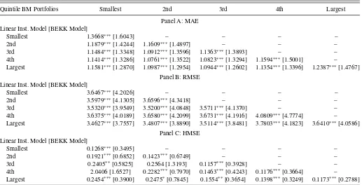
Table 6 provides element-wise comparisons for the MAE, RMSE, and HMSE for both models in Panels A, B, and C, respectively. For each cell of the table we report the linear in-formation instrument model estimate above the BEKK estimate in brackets. Individual significance levels for the DM test that the two losses are equal are denoted with asterisks throughout. We observe that for all but one occurrence, the estimated loss for the linear information instrument is smaller than the com-parable BEKK loss. The single exception occurs for the covari-ance element between the smallest and the fourth BM portfolio using the HMSE loss function. In this case, although the es-timated loss is smaller for the BEKK model, the difference is not significant. In sum, we have strong element-wise evidence that the linear information instrument model offers superior performance.
Averaging the percentage improvement in our model relative to the BEKK model across all elements in the lower triangu-lar matrices of Table 6, we find our model outperforms by 17 and 12% using the MAE and RMSE, respectively. When using the HMSE, the average outperformance is nearly 60%. Using the Diebold–Mariano statistics, the linear information instrument model significantly outperforms the BEKK model for all element-wise comparisons at the 1% level using both the
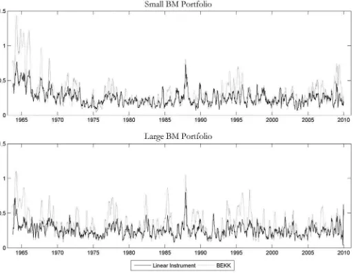
Figure 1. Estimation errors for the conditional variances of the small and large book-to-market (BM) portfolios. The solid (dotted) line is the 12-week moving average of absolute variance errors for the linear instrument (BEKK) model.
MAE and RMSE, and for most element-wise comparisons using HMSE.
Figures 1 and2 graphically display the performance of the linear instrument model and the BEKK model over time. In both panels of Figure 1, we plot the absolute differences between the estimated conditional variance series and the true variance series for both models. To dampen the short-term variability in the series, we calculate a moving average of the current and previous 11 absolute differences. The upper panel reports the moving average of absolute differences for the smallest book-to-market portfolio for each model. The lower panel reports the same quantities for the largest book-to-market portfolio. We note that the average absolute disturbances are typically smaller for the linear instrument model. Further, we do not observe any systematic impact suggesting that the BEKK model better fits one of the series over any subperiod of the sample when compared to the linear instrument model.
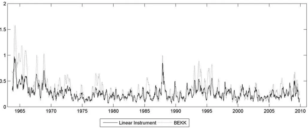
Because many financial applications and most covariance es-timation summary statistics treat all covariance terms as twice as important as variances, we also report the absolute errors across all unique covariance terms inFigure 2(ignoring the
di-agonal elements of the covariance matrix, as considered earlier). We again find evidence that the linear information instrument model has consistently smaller absolute errors than the BEKK model when describing covariances.
In the next empirical section, we present some finite sam-ple simulation results to examine the performance of the linear information instrument model and the BEKK model.
3.5 Finite Sample Simulations
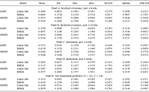
The previous results suggest that the linear information in-strument model performs well in our five portfolio example for a lengthy time series. In this section, we consider the generality of these findings to a subset of our assets, and for various finite samples.
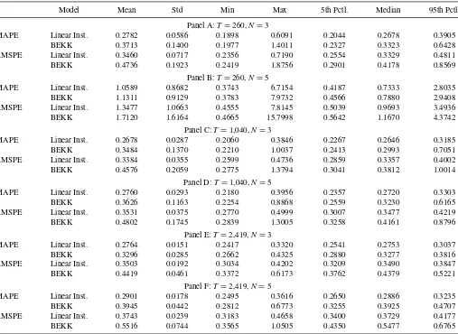
Our simulation experiment can be described as follows:
1. In all cases, we consider 1000 replications of the procedure described in Section 3.2 with T = 260, 1040, and 2419 andN =3 and 5. Given 52 weeks per year,T =260, and