Full Terms & Conditions of access and use can be found at
http://www.tandfonline.com/action/journalInformation?journalCode=ubes20
Download by: [Universitas Maritim Raja Ali Haji], [UNIVERSITAS MARITIM RAJA ALI HAJI
TANJUNGPINANG, KEPULAUAN RIAU] Date: 11 January 2016, At: 20:44
Journal of Business & Economic Statistics
ISSN: 0735-0015 (Print) 1537-2707 (Online) Journal homepage: http://www.tandfonline.com/loi/ubes20
Comment
Gabriele Fiorentini & Enrique Sentana
To cite this article: Gabriele Fiorentini & Enrique Sentana (2014) Comment, Journal of Business & Economic Statistics, 32:2, 193-198, DOI: 10.1080/07350015.2013.878661
To link to this article: http://dx.doi.org/10.1080/07350015.2013.878661
Published online: 16 May 2014.
Submit your article to this journal
Article views: 81
View related articles
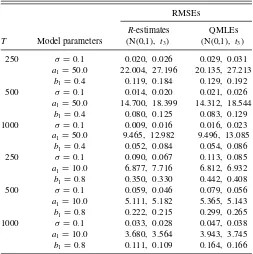
Table 1. Root mean squared errors forR-estimates and QMLEs of GARCH model parameters when the noise distribution is N(0,1) and
standardizedt3
RMSEs
R-estimates QMLEs
T Model parameters (N(0,1), t3) (N(0,1), t3)
250 σ =0.1 0.020, 0.026 0.029, 0.031
a1=50.0 22.004, 27.196 20.135, 27.213
b1=0.4 0.119, 0.184 0.129, 0.192
500 σ =0.1 0.014, 0.020 0.021, 0.026
a1=50.0 14.700, 18.399 14.312, 18.544
b1=0.4 0.080, 0.125 0.083, 0.129
1000 σ =0.1 0.009, 0.016 0.016, 0.023
a1=50.0 9.465, 12.982 9.496, 13.085
b1=0.4 0.052, 0.084 0.054, 0.086
250 σ =0.1 0.090, 0.067 0.113, 0.085
a1=10.0 6.877, 7.716 6.812, 6.932
b1=0.8 0.350, 0.330 0.442, 0.408
500 σ =0.1 0.059, 0.046 0.079, 0.056
a1=10.0 5.111, 5.182 5.365, 5.143
b1=0.8 0.222, 0.215 0.299, 0.265
1000 σ =0.1 0.033, 0.028 0.047, 0.038
a1=10.0 3.680, 3.564 3.943, 3.745
b1=0.8 0.111, 0.109 0.164, 0.166
ARE in Equation (3) is 1.041 when the noise {εt}are N(0,1),
and ARE is 1.052 when the{εt}are standardizedt3 (Andrews
2012). Since the RMSEs inTable 1forR-estimation are mostly smaller than the corresponding values for QMLE, it appears the asymptotic relative efficiencies forR-estimation with respect to
non-Gaussian QMLE can be indicative of finite sample behavior for sample size 250≤T ≤1000.
3. CONCLUDING REMARKS
In Andrews (2012), the limiting distribution forR-estimators is given not only when the true parameter vector is in the in-terior of its parameter space and the estimators are asymptot-ically Normal, but also when some GARCH parameters are zero and the limiting distribution is non-Normal. The results are used to develop hypothesis tests for GARCH order selection (Andrews2012, sec. 3.2). SinceR-estimates are straightforward to compute and tend to be relatively efficient, I recommend
R-estimation be used not only for preliminary GARCH estima-tion, but also for order selection when the noise distribution is unknown. If further model accuracy is desired, residuals from
R-estimation can be used to identify one or more suitable noise distributions, and then the GARCH model can be estimated via QMLE/MLE.
REFERENCES
Andrews, B. (2012), “Rank-Based Estimation for GARCH Processes,” Econo-metric Theory, 28, 1037–1064. [191,192,193]
Berkes, I., and Horv´ath, L. (2004), “The Efficiency of the Estimators of the Parameters in GARCH Processes,”The Annals of Statistics, 32, 633–655. [191]
Bollerslev, T. (1986), “Generalized Autoregressive Conditional Heteroskedas-ticity,”Journal of Econometrics, 31, 307–327. [192]
Hall, P., and Yao, Q. (2003), “Inference in ARCH and GARCH Models With Heavy-Tailed Errors,”Econometrica, 71, 285–317. [191]
Jaeckel, L. A. (1972), “Estimating Regression Coefficients by Minimizing the Dispersion of the Residuals,”Annals of Mathematical Statistics, 43, 1449– 1458. [192]
Comment
Gabriele F
IORENTINIUniversit `a di Firenze and RCEA, I-50134 Firenze, Italy ([email protected])
Enrique S
ENTANACEMFI, E-28014 Madrid, Spain ([email protected])
The Gaussian pseudo-maximum likelihood (PML) estimators advocated by Bollerslev and Wooldridge (1992) among many others remain root-Tconsistent for the conditional variance pa-rameters of univariate generalized autoregressive conditional heteroscedasticity (GARCH) models with a zero conditional mean irrespective of the degree of asymmetry and kurtosis of the conditional distribution of the observed variables, so long as the first two conditional moments are correctly specified and the fourth conditional moments are bounded. Nevertheless, many empirical researchers prefer to specify a non-Gaussian paramet-ric distribution for the standardized innovations, which they use to estimate the conditional variance parameters by maximum likelihood (ML). The most important commercially available econometric packages have responded to this demand by offer-ing ML procedures that either jointly estimate the parameters
characterizing the shape of the assumed distribution or allow the user to fix them to some prespecified values (see, e.g., the uni-variate ARCH sections of IHS Global Inc.2013and StataCorp LP2013).
However, while such ML estimators will often yield more ef-ficient estimators than Gaussian PML if the assumed conditional distribution is correct, they may end up sacrificing consistency when it is not, as shown by Newey and Steigerwald (1997). For that reason, Fan, Qi, and Xiu (2014) must be congratulated
© 2014American Statistical Association Journal of Business & Economic Statistics
April 2014, Vol. 32, No. 2 DOI:10.1080/07350015.2013.878661
Color versions of one or more of the figures in the article can be found online atwww.tandfonline.com/r/jbes.
for proposing a modification of parametric non-Gaussian PML estimators that achieve consistency even when the assumed dis-tribution is misspecified.
We shall center our comments around three main topics, in the hope that they will help popularize the use of these consistent estimation procedures among practitioners.
ASYMPTOTIC EQUIVALENCE WITH
THE CLOSED-FORM ESTIMATORS IN FIORENTINI AND SENTANA (2007)
In Fiorentini and Sentana (2007), we proposed very simple modifications of PML estimators of conditional mean and vari-ance parameters, which (subject to regularity) are consistent regardless of the degree of misspecification of the parametric conditional distribution used for estimation purposes. Although our setup was far more general, let us illustrate our proposal with the zero conditional mean, GARCH(1,1) model considered by Fan, Qi, and Xiu (2014):
Like them, we were interested in the consistent estimation of ϑ1=(γ , β)′ andϑ2 when the true distribution of ε∗t|It−1 is iid D(0,1;̺0), but possibly different from the distribution assumed for estimation purposes. In keeping with the notation of our article, we shall refer to the parameters of the estimated model asφ=(ϑ′,η′)′, whereϑ=(ϑ′
1, ϑ2)′, while we will use ϕ=(ϑ′,̺′)′ for the true parameter values. We also assume that η has been fixed to some value, sayη¯. To facilitate the comparison, the mapping between the notation in Fiorentini and Sentana (2007) and Fan, Qi, and Xiu (2014) is as follows: ϑ1=γ,ϑ2=σ2,λ∞(η¯)=ηf2,σ
⋄2
t =vt, andε∗t =εt.
The log-likelihood function for a sample ofT observations (ignoring initial conditions) takes the form
LT(φ)= −
As a result, the contribution of thetth observation to the score will be
which is effectively such that
E
In what follows, we shall refer to the ratio
λ∞(η)=ϑ2∞(η)/ϑ20 (3) as the “relative bias” in estimatingϑ2, so that
ǫt[ϑ10, ϑ2∞(η)]= Regardless of the value of η¯, we know from Newey and Steigerwald (1997) thatϑ1will be consistently estimated (sub-ject to regularity) because the law of iterated expectations and the serial independence ofε∗
t imply that
Therefore, we only need to correct the PML estimator ofϑ2. LetϑˆT =(ϑˆ
′
1T,ϑˆ2T)′ denote the PML estimators. For model
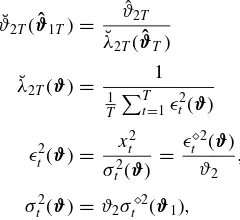
(1), the proposal in Fiorentini and Sentana (2007) simply boils down to replacing ˆϑ2T by
The rationale for this estimator comes from the fact that the Gaussian score forϑ2is simply
sϑ2t(ϑ,0)= 1 2ϑ2
[ǫ2
t(ϑ)−1].
If we regard this score as an additional influence function, we can obtain the asymptotic variance of ¯ϑ2T(ϑˆ1T), as well as its
asymptotic covariance withϑˆ1T. Nevertheless, we must
care-fully distinguish between theϑ2 parameter estimated with the potentially misspecified log-likelihood function and the param-eter estimated with the Gaussian score, which we shall refer to as ¯ϑ2to avoid confusion.
A numerically equivalent but even simpler to code estimator
which has the advantage that it uses the series of estimated con-ditional variances obtained as a by product of the ML estimation procedure.
In Eviews, the code would be:
equation return1.arch(1,1,tdist=7) y return1.makegarch condvar
series resid2std=yˆ2/condvar
scalar thetabar=c(1)*@mean(resid2std) scalar alphabarc=c(2)*@mean(resid2std)
Similarly, the Stata code would be
arch y, noconstant arch(1/1) garch(1/1) distribution(t 7)
predict condvar, variance
gen double resid2std2 = (yˆ2)/condvar summarize resid2std2
scalar invlambdabar = r(mean) matrix garchcoeffs = e(b)
scalar alphabar = invlambdabar* garchco-effs[1,1]
scalar thetabar = invlambdabar* garchco-effs[1,3]
In Fiorentini and Sentana (2007), we did not formally study the statistical properties of this estimator in detail. Somewhat remarkably, it turns out that our consistent estimators of ϑ1 and ϑ2, ϑˆ1T and ˘ϑ2T(ϑˆ1T), are asymptotically equivalent to
the three-step estimators proposed by Fan, Qi, and Xiu (2014). A formal proof of this result can be found in Fiorentini and Sentana (2013). In this regard, it is important to emphasize that given that the W(ϑ10;ϕ0) vector defined in (5) will generally be different from0in the GARCH model (1), ˘ϑ2T(ϑˆ1T) will be
more efficient than its Gaussian PML counterpart if and only if
ˆ
ϑ1T is in turn more efficient than the corresponding Gaussian
PMLE.
One final remark. It would be straightforward to conduct a test of consistency of the uncorrected PML estimators ofϑ based on the comparison between the estimator ofλ∞(η¯)in (7) and 1. We are currently investigating the relationship of such a test to the Hausman tests proposed in Fiorentini and Sentana (2007).
ESTIMATING THE SHAPE PARAMETERS TOGETHER WITH THE CONDITIONAL VARIANCE PARAMETERS
The ML estimators considered by Fan, Qi, and Xiu (2014), as well as the estimators considered in our previous point, are equality restricted estimators, in the sense that they fix the shape parameters to some prespecified valueη¯. As explained
by these authors, though, the resulting estimators are not nec-essarily more efficient than the Gaussian PML estimators, the obvious counterexample being an estimator that fixes η to a nonzero value when the true distribution is in fact Gaussian.
If we knew the true distribution of ε∗
t, but still decided to
use the wrong log-likelihood function, we could minimize the asymptotic variance ofϑˆ1T(η) with respect toηto achieve
ef-ficiency gains over the Gaussian case. In practice, we could estimate the required expressions by means of sample analogs with the unknown innovations replaced by estimated ones, and then chooseηas the minimizer of the estimated asymptotic vari-ance, along the lines of Francq, Lepage, and Zakoian (2011). The asymptotic distribution of the resulting estimators of ϑ1, ϑ2, andηdeserves further investigation.
Given existing software, though, practitioners are more likely to estimate the shape parameters jointly with the GARCH pa-rameters by ML (see again IHS Global Inc.2013and StataCorp LP2013).
Let
sηt(φ)= ∂lnf[ǫt(ϑ);η] ∂η
denote the log-likelihood score with respect toη. We can define its pseudo-true valueη∞from the equation
E{sηt[ϑ10, ϑ2∞(η∞),η∞]|ϑ0,̺
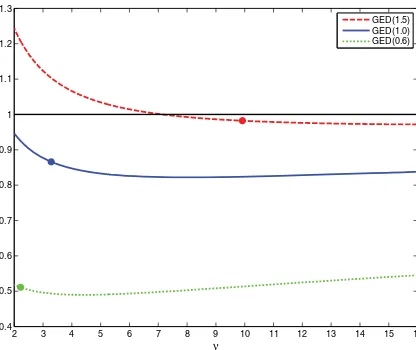
An obvious question at this stage is whether there are any efficiency gains in estimating η in this manner. The results in Amengual and Sentana (2010) and Fiorentini and Sentana (2010) suggest that one would expect to obtain estimators ofϑ1 more efficient than their Gaussian PML counterparts by simul-taneously estimatingη, at least when the pseudo-log-likelihood function nests the Gaussian one. We have assessed this conjec-ture when the distribution used for estimation purposes is a Stu-dent’stbut the true distribution is a generalized error distribution (GED), also known as the generalized Gaussian distribution.
Figure 1, which reports the efficiency of the estimators ofϑ1 for fixed degrees of freedomνrelative to the Gaussian PMLE, confirms our conjecture since the latter is always worse than the unrestricted ML estimator that simultaneously estimates η= ν−1, whose pseudo-true values are indicated by thick dots.
It is also interesting to assess whether the consistent esti-mator of ϑ2 entails any efficiency loss when the distribution assumed for estimation purposes is correct. Obviously, the esti-mators ofϑ1are fully efficient in that case, but ˘ϑ2T(ϑˆ1T) will
be generally inefficient relative to ˆϑ2T because it is based on the
Gaussian score. For illustrative purposes, we have computed this efficiency loss for the case in which the true and estimated distribution is a Student’stwith unknown degrees of freedom. Given that the fourth moment of this distribution diverges to infinity as the number of degrees of freedom converges to 4 from above, the asymptotic efficiency loss of ˘ϑ2T(ϑˆ1T) can be
made arbitrarily large. Nevertheless, as soon as the true degrees of freedom exceed 4.6, the efficiency loss is just 5%, and in fact it becomes negligible forν >6.
2 3 4 5 6 7 8 9 10 11 12 13 14 15 16 0.4
0.5 0.6 0.7 0.8 0.9 1 1.1 1.2 1.3
ν
GED(1.5) GED(1.0) GED(0.6)
Figure 1. Relative efficiency oft-based PMLE versus Gaussian PMLE.
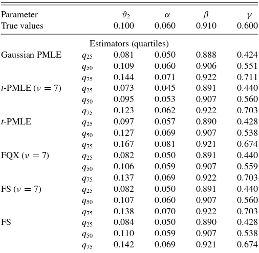
We have also carried out a simple Monte Carlo exercise to assess the extent to which those asymptotic gains accrue in fi-nite samples too. Our design, though, is different from the one in Fan, Qi, and Xiu (2014) because we wanted it to resemble more closely the typical estimates obtained in practice. To select realistic true parameter values, we have fitted a GARCH(1,1) model to the weekly (Wednesday to Wednesday) geometric returns of the Euro/U.S. $ exchange rate between the end of De-cember 2004 and the beginning of October 2013, a period over which the drift is negligible (the€/$ rate was 1.3608 on 2004-12-29 and 1.3515 on 2013-10-02, which justifies the zero drift assumption). On that basis, we have simulated a Laplace model in which β0=0.91 andϑ20=0.1 so that we can easily map γ0=0.6 to the value of the usual ARCH parameterα0=0.06. For the sake of completeness, we have considered six different estimators: Gaussian PMLE, Student’st-based PMLE withν re-stricted to 7, unrere-stricted Student’st-based PMLE, Fan, Qi, and Xiu (2014) three-step procedure withνrestricted to 7, Fiorentini and Sentana (2007) procedure withνrestricted to 7, and finally the unrestricted version of Fiorentini and Sentana (2007) that simultaneously estimatesη. For the purposes of maximizing the Student’st log-likelihood function, we have followed the nu-merical procedures in Fiorentini, Sentana, and Calzolari (2003). The results presented inTable 1confirm our previous com-ments. In particular, the consistent estimators of Fan, Qi, and Xiu (2014) and Fiorentini and Sentana (2007) mitigate the
notice-able biases inϑ2andαinduced by the unrestricted and restricted Student’st-based PMLEs. Moreover, they also have some mi-nor efficiency gains in the estimation ofβandγrelative to the Gaussian PMLE. Somewhat surprisingly, though, all the estima-tors ofγ show downward biases, which nevertheless become much smaller in larger sample sizes. The potential association between those finite sample biases and the high value of the “persistence” parameterα+βdeserves further investigation.
EXTENSIONS TO MORE GENERAL MODELS
As we mentioned before, the closed-form estimators in Fiorentini and Sentana (2007) apply far more generally, as they cover not only univariate models with nonzero conditional means, but also multivariate models. An important univariate example would be the asymmetric GARCH-M model consid-ered by Sun and Stengos (2006):
rMt =σt⋄(ϑ1)ξt
ξt =ϑ3+ϑ2εt∗
σ⋄
t(ϑ1)=1+σt⋄−1(ϑ1) [γf(ξt−1)+β] f(ξt−1)= |ξt−b| −c(ξt−b)
ε∗
t|It−1∼iid(0,1) with density functionf(ε;η) ⎫ ⎪ ⎪ ⎪ ⎪ ⎬ ⎪ ⎪ ⎪ ⎪ ⎭
(9)
for the excess returns of some financial asset,rMt, whereϑ1= (γ , β, b, c). If both the true and assumed distributions of ε∗
t
are symmetric, the results in Newey and Steigerwald (1997)
Table 1. Monte Carlo experiment. True distribution: Laplace (GED(1.0))T=2000; NREPS=10,000
Parameter ϑ2 α β γ
True values 0.100 0.060 0.910 0.600
Estimators (quartiles)
Gaussian PMLE q25 0.081 0.050 0.888 0.424
q50 0.109 0.060 0.906 0.551
q75 0.144 0.071 0.922 0.711
t-PMLE (ν=7) q25 0.073 0.045 0.891 0.440
q50 0.095 0.053 0.907 0.560
q75 0.123 0.062 0.922 0.703
t-PMLE q25 0.097 0.057 0.890 0.428
q50 0.127 0.069 0.907 0.538
q75 0.167 0.081 0.921 0.674
FQX (ν=7) q25 0.082 0.050 0.891 0.440
q50 0.106 0.059 0.907 0.559
q75 0.137 0.069 0.922 0.703
FS (ν=7) q25 0.082 0.050 0.891 0.440
q50 0.107 0.060 0.907 0.560
q75 0.138 0.070 0.922 0.703
FS q25 0.084 0.050 0.890 0.428
q50 0.110 0.059 0.907 0.538
q75 0.142 0.069 0.921 0.674
imply that one can consistently estimate the conditional mean parameterϑ3together withϑ1by PML. As forϑ2, expression (6) will remain consistent in that context too.
For general, possibly asymmetric distributions, the non-Gaussian PMLE ofϑ1will be consistent, while consistent esti-mators ofϑ2andϑ3can be obtained as the sample variance and mean, respectively, of the “standardized” innovations
ǫt⋄(ϑ1)= xt
σt⋄(ϑ1) .
Presumably, the Fan, Qi, and Xu (2014) three-step approach could be extended to cover model (9) too by estimating in their intermediate step a location parameter jointly with a scaling one. Our conjecture is that such an estimator would also be asymptotically equivalent to ours.
The inclusion of means in multivariate models also allowed us to cover many empirically relevant applications beyond ARCH models, which have been the motivating example for most of the existing work. In particular, our results apply to condition-ally homoscedastic, dynamic linear models, such as VaRs or multivariate regressions, which remain the workhorse in empir-ical macroeconomics and asset pricing contexts. For example, another rather popular model is the market model
rt =ψ
3+ψ1rMt+ 12/2ε∗t,
where rt denotes the excess returns on a vector of N as-sets. In this context, one can consistently estimate the beta coefficients ψ1 by non-Gaussian ML, while consistent esti-mators of 2 andψ3 can be obtained as the sample covari-ance matrix and mean vector, respectively, of the residuals ǫ⋄t(ψ1)=rt−ψ
1rMt. Again, the Fan, Qi, and Xu (2014)
three-step approach should extend to these multivariate models, al-though the second step would involve a numerical optimization overN(N+3)/2 parameters.
As explained by Fiorentini and Sentana (2007), substantial simplifications could be achieved when both the true and
esti-mated distributions are elliptically symmetric, since in that case the inconsistency is limited to a single overall scale parameter.
OTHER COMMENTS
The focus of the Fan, Qi, and Xiu (2014) article is the con-sistent estimation of the parametersϑ=(ϑ′1, ϑ2). However, the usual parameterization of a GARCH(1,1) model such as (1) would be
σt2(θ)=ω+αxt2−1+βσt2−1(θ), whereθ=(ω, α, β)′,ω=ϑ
2, andα=ϑ2γ. Fiorentini and Sen-tana (2013) obtained expressions for the asymptotic standard errors for the consistent estimator ofαgiven by ˘ϑ2T(ϑˆ1T)·γˆT
by means of the delta method.
One of the reasons why practitioners prefer to use non-Gaussian distributions for estimating GARCH models is that they are often not only interested in the conditional variance of the process, but also in other features of the conditional distribu-tion, such as its quantiles, which are required for the computation of commonly used risk management measures such as VaR. The consistent estimators discussed by Fan, Qi, and Xiu (2014) can improve upon the sequential estimators of the shape parameters discussed in Amengual, Fiorentini, and Sentana (2013), which rely on the Gaussian PMLEs ofϑ.
Finally, let us conclude by congratulating the authors once more for their work.
ACKNOWLEDGMENTS
Sentana gratefully acknowledges financial support from the Spanish Ministry of Science and Innovation through grant ECO 2011-26342, while Fiorentini acknowledges funding from MIUR PRIN MISURA - Multivariate models for risk assess-ment.
REFERENCES
Amengual, D., Fiorentini, G., and Sentana, E. (2013), “Sequential Estimators of Shape Parameters in Multivariate Dynamic Models,”Journal of Econo-metrics, 177, 233–249. [197]
Amengual, D., and Sentana, E. (2010), “A Comparison of Mean-Variance Effi-ciency Tests,”Journal of Econometrics, 154, 16–34. [195]
Bollerslev, T., and Wooldbridge, J. M. (1992), “Quasi-Maximum Likelihood Estimation and Inference in Dynamic Models With Time Varying Covari-ances,”Econometric Reviews, 11, 143–172. [193]
Fan, J., Qi, L., and Xiu, D. (2014), “Quasi-Maximum Likelihood Estimation of GARCH Models With Heavy-Tailed Likelihoods,”Journal of Business and Economic Statistics, 32, 178–191. [193,194,195,196,197]
Fiorentini, G., and Sentana, E. (2007), “On the Efficiency and Con-sistency of Likelihood Estimation in Multivariate Conditionally Het-eroskedastic Dynamic Regression Models,” CEMFI Working Paper 0713. [194,195,196,197]
——— (2010), “New Testing Approaches for Mean-Variance Predictability,” Mimeo, CEMFI. [195]
——— (2013), “Consistent Non-Gaussian Pseudo Maximum Likelihood Esti-mators,” Mimeo, CEMFI. [197]
Fiorentini, G., Sentana, E., and Calzolari, G. (2003), “Maximum Likelihood Estimation and Inference in Multivariate Conditionally Heteroskedastic Dy-namic Regression Models With StudenttInnovations,”Journal of Business and Economic Statistics, 21, 532–546. [196]
Francq, C., Lepage, G., and Zakoan, J.-M. (2011), “Two-Stage Non Gaussian QML Estimation of GARCH Models and Testing the Efficiency of the Gaussian QMLE,”Journal of Econometrics, 165, 246–257. [195]
IHS Global Inc. (2013),Eviews 8: Command and Programming Reference, Irvine, CA: IHS Global Inc. [193,195]
Newey, W. K., and Steigerwald, D. G. (1997), “Asymptotic Bias for Quasi-Maximumlikelihood Estimators in Conditional Heteroskedasticity Models,” Econometrica, 65, 587–599. [193,194,196]
StataCorp LP. (2013),STATA Time Series Reference Manual Release 13, College Station, TX: Stata Press. [193,195]
Sun, Y., and Stengos, T. (2006), “Semiparametric Efficient Adaptive Estima-tion of Asymmetric Garch Models,”Journal of Econometrics, 133, 373– 386. [196]
Comment
Christian F
RANCQand Jean-Michel Z
AKO¨
IANCREST, 92245 Malakoff Cedex, France; Universit ´e Lille 3, 59653 Villeneuve d’Ascq Cedex, France ([email protected]; [email protected])
In this interesting article, the authors developed and studied a non-Gaussian quasi-maximum likelihood (NGQML) method for estimating GARCH(p, q) models. The standard Gaussian QML estimator for generalized autoregressive conditional het-eroscedasticity (GARCH) is well known to be consistent and asymptotically Gaussian under mild conditions but it may lack accuracy when the underlying innovations density is far from the Gaussian. This article proposes to use a three-step method in which the unknown density is approximated via a rescaling of a given likelihood density. The GQML is used in a first step to provide approximations of the innovations, which are used in a second step to appropriately fit the scaling factor. The third step involves a new QML optimization, now using the density emerging from the second step.
In this comment, we would like to discuss two points, one concerning the practical implementation of the method and the comparison with the two-step quasi-maximum likelihood es-timate (hereafter 2QMLE) proposed by Francq, Lepage, and Zako¨ıan (2011), and the other one concerning the behavior of the method when strict stationarity does not hold.
1. PRACTICAL IMPLEMENTATION AND A COMPARISON
To explain the difference between the 2QMLE and the three-step NGQMLE that is proposed here, let us assume a GARCH(1,1) modelxt =vtεt, with
v2t(θ0)=c0+a0xt2−1+b0vt2−1(θ0), θ0=(c0, a0, b0)′. (1) The 2QMLE is based on a density belonging to the class of the generalized Gaussian (GG) distributions
fβ(x)∝e−|x|
β/β
, β >0. The two steps of this method are as follows:
1. Compute the estimator
θ∗T =c∗T,aT∗,b∗T′=arg min θ∈
T
t=1 '
logvt(θ)+
|xt|β
βvtβ(θ)
( .
2. From the residualsǫt∗=xt/vt(θ
∗
T),t =1, . . . , T, compute
the 2QMLE
θ∗T =μˆ2∗,Tc∗T,μˆ∗2,Ta∗T,b∗T, where ˆμ∗
s,T =T
−1T
t=1|ǫ∗t|sfors >0.
When the NGQMLE is based on the same densityfβ(x), the
three steps are as follows:
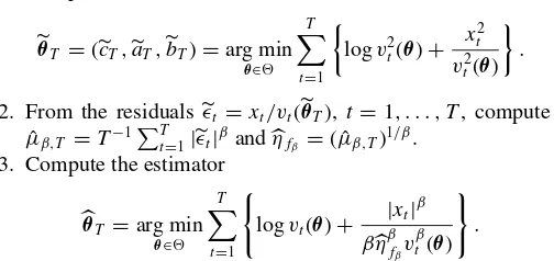
1. Compute the GQML estimator
θT =(cT,aT,bT)=arg min
θ∈ T
t=1
logv2t(θ)+ x 2 t
v2t(θ)
.
2. From the residualsǫt=xt/vt(θT),t =1, . . . , T, compute
ˆ
μβ,T =T−1Tt=1|ǫt|βandηfβ =( ˆμβ,T) 1/β.
3. Compute the estimator
θT =arg min
θ∈ T
t=1 '
logvt(θ)+
|xt|β
βηβf βv
β t(θ)
( .
As shown by the authors of the present article, the two esti-matorsθ∗T andθT have the same asymptotic distribution. The
2QMLE is, however, a little bit simpler because it involves only one numerical optimization. Moreover, the finite-sample dis-tributions of the two estimators may be significantly different. To see this, we generated 1000 independent replications of a GARCH(1,1) model (1) in which εt follows the Student
dis-tribution with parameterν=4.5 (rescaled in such a way that Eε21 =1), and we applied the NGQML and 2QML withβ=1. Table 1shows that for the large sample sizeT =10,000, the 2QMLE and NGQMLE are equivalent, and they are both more accurate than the GQMLE. For small or moderate sample sizes (i.e.,T =500 orT =2000), the 2QMLE and NGQMLE are equivalent for the estimation ofa0, but the root mean square error (RMSE) of estimation ofc0andb0 is clearly smaller for
© 2014American Statistical Association Journal of Business & Economic Statistics
April 2014, Vol. 32, No. 2 DOI:10.1080/07350015.2013.879829
Color versions of one or more of the figures in the article can be found online atwww.tandfonline.com/r/jbes.