00074918.2014.938405

(1)

Full Terms & Conditions of access and use can be found at

http://www.tandfonline.com/action/journalInformation?journalCode=cbie20

Download by: [Universitas Maritim Raja Ali Haji] Date: 17 January 2016, At: 23:28

Bulletin of Indonesian Economic Studies

ISSN: 0007-4918 (Print) 1472-7234 (Online) Journal homepage: http://www.tandfonline.com/loi/cbie20

Does Economic Growth Really Benefit the Poor?

Income Distribution Dynamics and Pro-poor

Growth in Indonesia

Indunil De Silva & Sudarno Sumarto

To cite this article: Indunil De Silva & Sudarno Sumarto (2014) Does Economic Growth Really Benefit the Poor? Income Distribution Dynamics and Pro-poor Growth in Indonesia, Bulletin of Indonesian Economic Studies, 50:2, 227-242, DOI: 10.1080/00074918.2014.938405

To link to this article: http://dx.doi.org/10.1080/00074918.2014.938405

Published online: 30 Jul 2014.

Submit your article to this journal

Article views: 530

View related articles

View Crossmark data

(2)

* TNP2K = Tim Nasional Percepatan Penanggulangan Kemiskinan (National Team for the Acceleration of Poverty Reduction), Ofice of the Vice-President. The views expressed in this article are the sole responsibility of the authors and do not necessarily relect the views of TNP2K.

DOES ECONOMIC GROWTH REALLY BENEFIT THE POOR?

INCOME DISTRIBUTION DYNAMICS AND PRO-POOR

GROWTH IN INDONESIA

Indunil De Silva and Sudarno Sumarto*

TNP2K, Jakarta

We explore the nexus between poverty, inequality, and economic growth in Indone-sia between 2002 and 2012, using several pro-poor growth concepts and indices to determine whether growth in this period beneited the poor. Our regression-based decompositions of poverty into growth and redistribution components suggest that around 40% of inequality in total household expenditure in Indonesia was due to variations in expenditure by education characteristics that persisted after control-ling for other factors. We ind that economic growth in this period beneited house -holds at the top of the expenditure distribution, and that a ‘trickle down’ effect saw the poor receive proportionately fewer beneits than the non-poor. If reducing poverty is one of the Indonesian government’s principal objectives, then policies designed to spur growth must take into account the possible impacts of growth on inequality.

Keywords: economicgrowth, poverty, inequality, pro-poor, decomposition

JEL classiication: D31, D63, I32

INTRODUCTION

Indonesia has in recent years used its strong and sustained economic growth to accelerate its rate of poverty reduction. Yet while poverty fell by 34% between 2002 and 2012, Indonesia’s Gini coeficient (a common indicator of income in equality) increased by 30%, which suggests that rising inequality dampened most of the poverty-reducing effects of growth. Fiscal decentralisation, labour market reforms, state-led development, and social protection policies largely reallocated labour and unemployment, increasing wage inequalities and altering expenditure patterns. Changes in demographics, human capital, and the sectoral composition of growth (from agriculture to industry and services), driven in part by increased global integration and rural–urban migration, are the most probable causes of rising inequality in Indonesia.

(3)

228 Indunil De Silva and Sudarno Sumarto

Rising inequality can produce violent protests and other forms of collective behaviour that can impede economic growth. Even when social tensions do not result in violence, perceptions of the inequitable effects of policy reform can ham-per a government’s ability to introduce the reforms needed for economic growth (Coudouel, Dani, and Paternostro 2006). Indonesia faces the dificulty of acceler-ating its rate of poverty reduction while adopting a pro-poor growth framework that allows the poor to beneit disproportionately more than the rich from eco-nomic growth (and thereby curbs rising inequality). Setting targets for greater equity in policymaking is intricate and not straightforward, but its complexity should not become a pretext for inertia in addressing one of Indonesia’s priorities for development. Thus, in this context, it is particularly important to examine the nexus between poverty, inequality, and economic growth in Indonesia.

Many researchers recognise that the effectiveness of growth in reducing poverty is tied to inequality (Jain and Tendulkar 1990; Datt and Ravallion 1992; Kakwani 2000; McCulloch, Cherel-Robson, and Baulch 2000; Shorrocks 2011). According to Ravallion (2004), the distribution-corrected rate of growth in average income can be expressed as initial equality times the rate of growth: for a given rate of growth, relatively more equal societies will have higher distribution-corrected rates of growth than relatively less equal societies. Hence the impacts on poverty of a given level of growth will be greater for higher rates of distribution-corrected growth. Other studies (Ferreira and Ravallion 2009; Fosu 2009; Banerjee and Dulo 2005; World Bank 2005) show that rising inequality reduces the growth elastic-ity of poverty reduction and creates poverty and inequalelastic-ity ‘traps’ that restrict economic growth. Klasen and Misselhorn (2008) use a semi-elasticity approach in examining the relationship between income growth and distributional change in the Foster–Greer–Thorbecke poverty index. They ind that growth in mean incomes has vastly different results in different circumstances—and, in particular, that high levels of initial inequality greatly lessen the contribution of growth to poverty reduction in countries whose mean income is not far above the poverty line. Dollar, Kleineberg, and Kraay (2013), using a global dataset spanning 118 countries, ind that just over three-quarters of the improvement in the incomes of the poorest 40% was attributable to increases in average incomes—that is, that this improvement came mainly from growth.

Timmer (2004) investigates economic growth in Indonesia during 1960–90. He inds that growth was instrumental in reducing poverty in this period, and that Indonesia experienced both ‘relative’ and ‘absolute’ pro-poor growth. He con-cludes that there were no episodes in which the poor were absolutely worse off during sustained periods of economic growth. Suryadarma et al. (2005) show that high levels of inequality reduced the growth elasticity of poverty in Indonesia during 1999–2002. They ind that Indonesia’s attempts to reduce poverty suc-ceeded because inequality in 1999 was at its lowest level in 15 years, which meant that growth had a greater effect on poverty reduction. Suryahadi, Suryadarma, and Sumarto (2009) examine the relationship between economic growth and pov-erty reduction by differentiating growth and povpov-erty into their sectoral composi-tions and locacomposi-tions. They ind that the most effective way to accelerate poverty reduction is to focus on the growth of rural agriculture and urban services. Surya-hadi, Hadiwidjaja, and Sumarto (2012) assess the relationship between economic growth and poverty reduction in Indonesia before, during, and after the 1997–98 Asian inancial crisis. They ind that growth in the services sector contributed the

(4)

most to poverty reduction, whereas growth in the agriculture sector beneited only poor rural households.

In this article we attempt to determine whether Indonesia’s economic growth during 2002–12 was pro-poor. Many studies have analysed poverty and in equality in Indonesia, but there is a dearth of microeconomic literature on recent pro-poor growth and regression-based redistribution decompositions. Our micro-level dynamic analysis of the nexus between poverty, inequality, and economic growth aims to deine how much of the decline in poverty in this period was imputable to changes in mean income and how much was imputable to changes in inequal-ity. We also examine the link between different socio-economic characteristics and total inequality, by assessing to what extent the returns to education brought about by Indonesia’s global integration and labour market reforms contributed to total consumption inequality (after controlling for the household, industry, employment, and regional characteristics that could affect welfare). Our analysis draws on data from the 2002 and 2012 rounds of the National Socio-economic Sur-vey (Susenas) and uses national poverty lines (Rp 113,064 per capita per month for 2002 and Rp 248,707 per capita per month for 2012).

POVERTY AND INEQUALITY IN INDONESIA SINCE THE 1970s

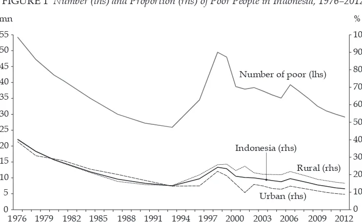
Indonesia has made remarkable progress in tackling poverty over the last 40 years, despite impediments such as the Asian inancial crisis in the late 1990s. The crisis aside, sustained growth in recent years—made possible by improvements in democracy, rapid political reforms, largely effective economic policies, and an enabling economic and institutional environment—have seen Indonesia trans-form its poor, largely rural economy into a dynamic, industrialising one. From a macroeconomic perspective, Indonesia has been a model of successful economic development in Southeast Asia since the 1970s. This period of sustained growth has brought about large improvements in social welfare; it has been one of Indo-nesia’s most successful episodes of poverty reduction, with the poverty incidence declining from 44% in 1976 to 13% in 1993. In general, between 1999 and 2012 the poverty headcount index (as measured against the national poverty line) fell gradually.

The Asian inancial crisis, which began in July 1997 with the devaluation of the Thai baht, was transmitted rapidly to Indonesia by way of a speculative attack on the Indonesian rupiah. In August the rupiah collapsed and inlation soared; food prices outpaced general headline prices; and a social and economic crisis exploded into a political crisis, with the then president, Soeharto, eventually being forced to resign in May 1998. By 1999, Indonesia’s poverty rate had reached 24% and other socio-economic outcomes, such as the schooling drop-out rate, had also increased. By 2004, however, poverty had fallen to below pre-crisis levels, to less than 17% (igure 1).

Later, in 2006, poverty increased again, with the headcount index rising to 18% from 16% in 2005. This time it was due primarily to the government’s decision to increase the domestic price of fuel by an average of around 120%, and to a sharp increase in the price of rice between February 2005 and March 2006. In recent years, in spite of sustained economic growth, the rate of poverty reduction has begun to slow, largely because of the changing nature of poverty. As a country’s poverty incidence falls to about 10%, it becomes dificult to reduce it further. At

(5)

times when poverty was about 25%, many households were just below the pov-erty line, and hence only a slight increase in income was needed to push them out of poverty. But the nature of poverty has changed, with many households far below the poverty line and others clustered on or just above the poverty line and at risk of falling back into poverty (Suryahadi et al. 2011; Dartanto and Nurkholis 2013).

Poverty in contemporary Indonesia has three salient features. First, many households are clustered around the national income poverty line, rendering them vulnerable to poverty. It is estimated that almost half of Indonesia’s pop-ulation lives on less than 15,000 rupiah (about $1.30) per day, and, as a result, small shocks can drive near-poor households into poverty. Thus it is common for households in Indonesia to churn into and out of poverty. Evidence from panel data suggests that during 2007–9 more than half of the poor in one year were not poor the previous year (Dartanto and Nurkholis 2013). Second, the income and monetary poverty measures do not always capture the true picture of poverty in Indonesia; many households that are not income poor could be categorised as multidimensional poor, owing to lack of access to basic services and poor human opportunities and development outcomes (Wardhana 2010). Third, given Indone-sia’s vast size and heterogeneity, regional disparities are an entrenched feature of poverty in the country and national averages mask stark differences. The poverty incidence in some of the outlying provinces, such as Papua, was as high as 31% in 2012, compared with less than 4% in Jakarta (BPS 2013).

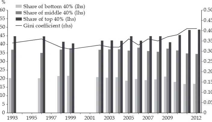
Low levels of inequality in periods of high economic growth have generally allowed Indonesia to reduce absolute poverty in the last three decades. Figure 2 shows movements in the expenditure shares and Gini coeficient during 1993– 2012. Notwithstanding this progress in reducing poverty, inequality in Indonesia

FIGURE 1 Number (lhs) and Proportion (rhs) of Poor People in Indonesia, 1976–2012

Number of poor (lhs)

1976 1979 1982 1985 1988 1991 1994 1997 2000 2003 2006 2009 2012 0

Source: Data from the National Socio-economic Survey (Susenas).

(6)

FIGURE 2 Gini Coeficient and Expenditure Shares, 1993–2012

1993 1995 1997 1999 2001 2003 2005 2007 2009 2012 0

Source: Data from the National Socio-economic Survey (Susenas).

Note: Gini coeficients are expenditure-based and calculated from Susenas data. Expenditure shares are shares in total household expenditure. Susenas signiicantly underestimates total consumer expenditure according to the national accounts. Assuming that expenditure by high-income house-holds is under-surveyed, Susenas overestimates the shares of low- and middle-income earners in total household expenditure. See Hill (1996, 195).

increased between 2002 and 2012. During 1993–96, prior to the Asian inancial crisis, the Gini coeficient increased from 0.34 to 0.36. In 1999, it dropped to a new low of 0.31—probably because the crisis hit high-income households dis-proportionately harder than it did other households, narrowing the income gap (Said and Widyanti 2002). This inluence may have been transmitted through large shifts in relative agricultural prices, which may have beneited those in the rural economy more than those in the more formal, urban economy (Tjiptoheri-janto and Remi 2001). In 2006, inequality began to increase. Although the Asian inancial crisis reduced inequality in Indonesia, from 2006 to 2012 the Gini coef-icient rose and the expenditure share, as measured by Susenas, of the bottom 40% decreased from 20% to 17%. In contrast, in the same period the consumption share of the top 20% increased from 42% to 49%. These changes suggest an extensive regressive redistribution of income from the great majority of the population to a very small elite.

ANALYTICAL FRAMEWORK AND METHODOLOGY

In examining the dynamics of pro-poor growth, we base our growth-redistribution decompositions and indices of pro-poorness on the methodologies of Datt and Ravallion (1992), Ravallion and Chen (2003), Kakwani and Pernia (2000), and Kakwani, Khandker, and Son (2003). Our decomposition of observed changes in poverty between 2002 and 2012 into growth and redistribution components

(7)

draws on the methodology of Datt and Ravallion (1992). The changes in poverty between 2002 (t–1) and 2012 (t) can be expressed as:

where P z

(

_;α

)

is the normalised Foster–Greer–Thorbecke index,_µ_{is mean} expend-iture, and z is the poverty line. The expression

P

represents the level of poverty in 2002 after its expenditures have been scaled by

µt µt−1to yield a distribution with mean µt while holding inequality constant.

The irst poorness measure is the ‘poverty equivalent growth rate’ pro-posed by Kakwani and Pernia (2000) and adopted by Kakwani, Khandker, and Son (2003) and Kakwani and Son (2008). This rate is based on the growth elasticity of poverty and is expressed as:

δ=dln

( )

θ γ ₌ 1

θ_γ 0 ∂∂yP H

∫ y

( )

p g

( )

p dp (2)

whereγ =dln

( )

_µ _{is the growth rate of mean expenditure and}_{g p}

( )

₌dln

(

x p

( )

)

is the growth rate of the expenditure of households at pth percentile. Thus δ is the percentage change in poverty headcount resulting from a growth rate of 1% in mean expenditure. It is always negative. Next, the poverty-equivalent growth rate,(P_EGR)₌γ*_{, can be expressed as:}

where φ=δ η is the pro-poor index derived by Kakwani and Pernia (2000). Our measures of poor growth are the growth incidence curve and the pro-poor growth (PPG) index proposed by Ravallion and Chen (2003). The growth incidence curve plots the cumulative share of the population against income growth of the ξth quantile when household expenditure is ranked in ascending order. It can be expressed as:

g_t

( )

ξ = expenditure of µ. We then deine the PPG measure by the mean growth rate of the

household expenditure of the poor:

(8)

whereH_t₋1is the poverty headcount in the irst period. The rate of PPG, then, is

the change in the Watts index divided by the poverty headcount in the irst period. Last, we use the regression-based inequality decomposition techniques of Fields (2003) and Morduch and Sicular (2002) to answer two different types of questions. The regression-based decomposition methodology starts with an expenditure-generating equation:

where X is a vector of independent regressor variables capturing the exogenous determinants of expenditure, such as household demographics, education, employment, assets, infrastructure, and spatial effects; β is the vector of estimated regression coeficients; andεis an n-vector of residuals.

Following Shorrocks’s (1982) inequality decomposition, we use the regression estimates to construct the relative share of inequality attributed to componentX_k_:

S

kcan be interpreted as the share of inequality that can be attributed to the unequal distribution ofX_k_{across households.}

EMPIRICAL RESULTS

Between 2002 and 2012, poverty in Indonesia declined from 18% to 12% and the population under the poverty line reduced from 38.4 million to 29.1 million (table 1). Poverty was highest in the rural sector, followed by in the country as a whole and in the urban sector. The decrease in poverty in the urban sector was much greater than the decreases nationally and in the rural sector, which indicates that poverty did not fall in the sector in which it was most prevalent. Accord-ing to table 1 and igure 2, the Gini coeficient increased by 26%, from 0.31 to 0.39, between 2002 and 2012. The expenditure gap between the top and bottom quintiles of households increased substantially during this period. The bottom quintile received around 9.0% of all expenditure in 2002 and 7.5% in 2012, while the top quintile received 40.0% and 46.7%.

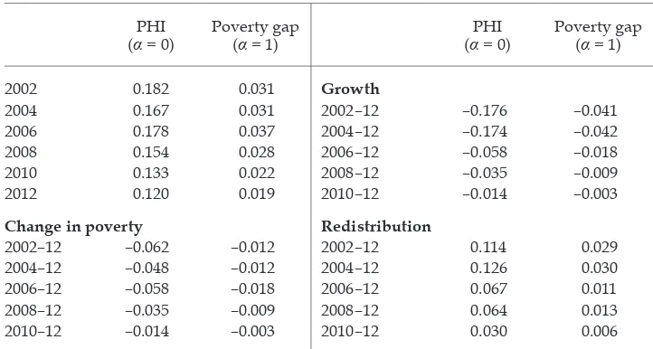
Table 2 decomposes the changes in Indonesia’s headcount poverty during 2002–12 into the effects of growth and of changes in inequality. In this period the changes in poverty were statistically signiicant and the effects of both growth and redistribution were great. The positive sign on the redistribution component indicates a negative impact on poverty reduction, owing to worsening inequal-ity—growth reduced poverty by around 17.5 percentage points, but the increase in inequality offset this reduction by 11.4 percentage points. Redistribution reduced growth by more than half, and poverty would have fallen by roughly 17 percentage points had inequality not increased. The aggravation of inequal-ity in Indonesia during these years weakened the effects of growth on poverty

(9)

TABLE 1 Proile of Poverty and Inequality, 2002 and 2012

Urban Rural Indonesia

2002 2012

Change

(%) 2002 2012

Change

(%) 2002 2012

Change (%)

Expenditure per

person (real $ ’000) 240 743 210 177 501 183 205 622 203 Theil index 0.21 0.34 62 0.11 0.20 82 0.17 0.30 76 Atkinson index 0.09 0.14 56 0.05 0.08 60 0.07 0.12 71 MLD index 0.18 0.27 50 0.10 0.16 60 0.15 0.24 60 Gini coeficient 0.33 0.40 21 0.25 0.30 20 0.31 0.39 27 Share of poverty (%) 35 36 5 65 64 –3 100 100 0 No. of poor (mn) 13.3 10.6 –20 25.1 18.5 –26 38.4 29.1 –24 PHI (α = 0) 14.5 8.8 –39 21.1 15.1 –28 18.2 12.0 –34 PGI (α = 1) 2.45 1.40 –43 3.60 2.4 –33 3.08 1.90 –38

Source: Authors’ calculations based on data from the National Socio-economic Survey (Susenas).

Note: MLD = mean logarithmic deviation. PHI = poverty headcount index. PGI = poverty gap index. Household per capita expenditure is adjusted for spatial price-level differences.

TABLE 2 Growth: Redistribution Decompositions, 2002–12

PHI

(α = 0) Poverty gap (α = 1) (α = 0) PHI Poverty gap (α = 1)

2002 0.182 0.031 Growth

2004 0.167 0.031 2002–12 –0.176 –0.041

2006 0.178 0.037 2004–12 –0.174 –0.042

2008 0.154 0.028 2006–12 –0.058 –0.018

2010 0.133 0.022 2008–12 –0.035 –0.009

2012 0.120 0.019 2010–12 –0.014 –0.003

Change in poverty Redistribution

2002–12 –0.062 –0.012 2002–12 0.114 0.029

2004–12 –0.048 –0.012 2004–12 0.126 0.030

2006–12 –0.058 –0.018 2006–12 0.067 0.011

2008–12 –0.035 –0.009 2008–12 0.064 0.013

2010–12 –0.014 –0.003 2010–12 0.030 0.006

Note: PHI = poverty headcount index.

(10)

reduction. Average expenditure increased substantially in both the urban and the rural sectors, but strong adverse redistribution effects cancelled out almost half of the positive effects of growth on poverty. Table 2 also gives the effects of growth and redistribution for four sub-periods between 2002 and 2012. The positive sign on the redistribution component signiies the negative impact of worsening ine-quality on poverty reduction during these sub-periods, and it is again evident that growth and redistribution had a considerable impact on poverty.

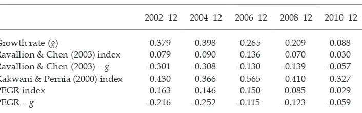
Table 3 provides estimates for Indonesia’s 2002–12 growth rate (denoted by the variable g), and for the three different pro-poor indices: the Ravallion and Chen (2003) index; the Kakwani, Khandker, and Son (2003) PEGR index; and the Kakwani and Pernia (2000) index. All three indices of absolute pro-poorness are statistically greater than zero, which means that the changes from 2002 to 2012 decreased absolute poverty. Ravallion and Chen’s PPG > 0 and the changes dur-ing 2002–12 are absolutely pro-poor while having irst-order dominance over the

initial distribution. However, since the PPG index is less than the growth rate of the population’s mean income, growth during this period cannot be deemed

relatively pro-poor, because the distributional shifts went against the poor. The PEGR index is greater than zero but less than the mean growth in population expenditure, and thus characterises a ‘trickle down’ effect (Kakwani, Khandker, and Son 2003) by which the poor beneited proportionately less from growth than did the non-poor. The PEGR shows that growth reduced poverty during 2002–12 but was accompanied by increasing inequality. Moreover, the estimates of Raval-lion and Chen’s (2003) PPG index minus g and of Kakwani, Khandker, and Son (2003) PEGR index minus g are all negative, indicating that growth was not rela-tively pro-poor. Thus we can infer that the growth rates of the incomes of the poor were not high enough to follow the growth rate in average income, and that the relative shares of the poor in total expenditure decreased during 2002–12. Simi-larly, all pro-poor indices displayed the same pattern of growth in all sub-periods, with distributional shifts working against the poor.

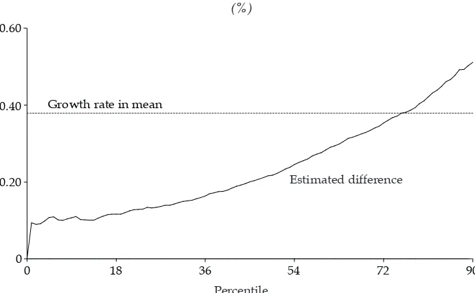
In igure 3, the growth incidence curve shows the distributive impact of growth between 2002 and 2012. The absolute change in expenditure is everywhere

TABLE 3 Pro-Poor Indices, 2002–12

2002–12 2004–12 2006–12 2008–12 2010–12

Growth rate (g) 0.379 0.398 0.265 0.209 0.088 Ravallion & Chen (2003) index 0.079 0.090 0.136 0.070 0.030 Ravallion & Chen (2003) – g –0.301 –0.308 –0.130 –0.139 –0.057 Kakwani & Pernia (2000) index 0.430 0.366 0.565 0.410 0.327

PEGR index 0.163 0.146 0.150 0.085 0.029

PEGR – g –0.216 –0.252 –0.115 –0.123 –0.059

Note: See text for deinitions of indices. g = the growth rate of real per capita household expenditure for each of the respective periods using the beginning year as the base year. PEGR = poverty-equivalent growth rate proposed by Kakwani and Pernia (2000); Kakwani, Khandker, and Son (2003); and Kak-wani, and Son (2008).

(11)

statistically positive, indicating that growth was absolutely pro-poor throughout the distribution. The growth incidence curve shows that there is irst-order domi-nance, which implies that poverty fell no matter where we draw the poverty line or what poverty measure we use within a broad class (Atkinson 1987; Foster and Shorrocks 1988). The growth incidence curve also shows that in reality very few households moved up along with the average growth rate of the economy. Growth in expenditure was very modest for the households in the 10th percentile, while, at the top, the 90th percentile experienced a signiicant increase in expenditure. Expenditure at the 10th percentile increased by only around 10% during 2002–12 (an average annual increase of 1%), whereas expenditure at the 90th percentile increased by around 50% (an average annual increase of 5%). The steep upward slope of the growth incidence curve implies that, in general, growth was accom-panied by rising inequality: the rate of expenditure growth of individuals in the upper expenditure percentiles was higher than that of the poor. Additionally, the proportional changes relative to the growth rate in mean expenditure also varied substantially across percentiles. Table 3 shows that the mean growth in expendi-ture was around 38%, which evidently exceeded the growth rates experienced by most Indonesians: the bottom four quintiles experienced below-average growth rates of expenditure. The evidence that inequality levels increased substantially between 2002 and 2012 is consistent with the fact that growth rates were not pro-portional across percentiles.

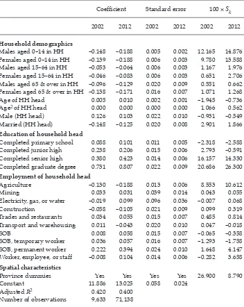
Table 4 provides the semi-log regression results and quantiies the importance of various contributors to inequality in Indonesia in 2002 and 2012. Columns 1 and 2 give the coeficients from a linear expenditure equation estimated by ordinary least squares for the full sample of households, and the columns 3 and 4 give stand-ard errors. Most of the estimated coeficients are highly statistically signiicant, with the expected signs. Per capita expenditure decreases with the number of

FIGURE 3 Growth Incidence Curve, 2002–12 (%)

Growth rate in mean

18 36 54 72 90

0 0 0.20 0.40 0.60

Estimated difference

Percentile

(12)

TABLE 4 Regression-Based Inequality Decompositions, 2002 and 2012

Coeficient Standard error 100 ×S_k

2002 2012 2002 2012 2002 2012

Household demographics

Males aged 0–14 in HH –0.148 –0.188 0.005 0.002 12.165 14.876 Females aged 0–14 in HH –0.139 –0.188 0.006 0.003 9.780 13.588 Males aged 15–64 in HH –0.053 –0.064 0.006 0.003 1.167 1.976 Females aged 15–64 in HH –0.046 –0.083 0.006 0.003 0.651 2.706 Males aged 65 & over in HH –0.096 –0.129 0.020 0.009 0.551 0.662 Females aged 65 & over in HH –0.138 –0.171 0.016 0.007 1.071 1.268 Age of HH head 0.005 0.010 0.002 0.001 –1.945 –0.736 Age2 _{of HH head} _0.000 _0.000 _0.000 _0.000 _1.066 _0.562

Male (HH head) 0.126 0.103 0.022 0.010 –0.931 –0.549 Married (HH head) –0.148 –0.125 0.020 0.008 2.901 1.866

Education of household head

Completed primary school 0.088 0.101 0.011 0.005 –2.318 –2.588 Completed junior high 0.238 0.206 0.015 0.006 2.793 –0.591 Completed senior high 0.380 0.423 0.014 0.006 16.157 14.330 Completed graduate degree 0.731 0.807 0.022 0.009 20.686 26.300

Employment of household head

Agriculture –0.130 –0.188 0.013 0.006 8.553 10.612

Mining 0.033 0.031 0.039 0.014 0.043 0.055

Electricity, gas, or water –0.019 0.099 0.096 0.036 –0.007 0.068

Construction –0.058 –0.105 0.021 0.009 0.099 0.319

Trades and restaurants 0.034 0.055 0.015 0.007 0.485 0.814 Transport and warehousing 0.011 –0.043 0.020 0.010 0.047 –0.018

SOB 0.008 0.058 0.015 0.007 –0.065 –0.358

SOB, temporary worker 0.036 0.057 0.016 0.007 –1.293 –1.758 SOB, permanent worker 0.222 0.394 0.024 0.010 1.648 4.147 Worker, employee, or staff –0.008 0.104 0.014 0.006 –0.282 3.658

Spatial characteristics

Province dummies Yes Yes Yes Yes 26.900 8.790

Constant 11.886 13.025 0.058 0.024

Adjusted R2 _0.420 _0.400

Number of observations 9,633 71,138

Note: Dependent variable is per capita household expenditure. S_k is deined in equation (7). HH = household. SOB = self-owned business.

household members and increases with the household head’s age. Expenditure is higher for urban and non-agricultural households. Education raises expenditure, and increasingly so for higher levels of education of the household head.

Table 4 also presents our decomposition results and answers the two questions raised by Fields (1998) and Morduch and Sicular (2002) in their proposed decom-position methodologies. First, given an expenditure-generating function estimated

(13)

by a standard semi-logarithmic regression, how much expenditure in equality is accounted for by, for example, education, employment, demographic, or spatial factors? Second, how much of the difference in income inequality between one date and another is accounted for by education, by potential employment char-acteristics, and by the other explanatory factors? Policymakers in Indonesia may beneit from knowing whether observed changes in inequality are due to changes in the returns to factors (such as education) or to changes in the distribution of factors of production (such as demographic characteristics).

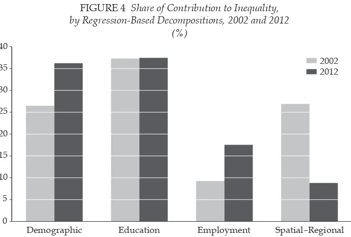
Figure 4 and table 4 (columns 5 and 6) of answer the above questions and summarise the overall group (demographic, education, employment, and spa-tial) contributions to inequality in 2002 and 2012. It is evident that differences in education, demographics, regional location, and employment across households have contributed substantially to total inequality. However, the differentials in expenditure by education characteristics were larger than by other factors. Theo-retically, greater education inequality should be associated with greater income inequality, because a higher level of education should ensure a higher income. Thus, differences in educational achievements imply differences in the ability to earn income, and, consequently, imply disparities in expenditure. During both 2002 and 2012, differences in expenditure related to the educational attainment of household heads contributed substantially (37%, on average) to overall inequal-ity, suggesting that education policies potentially have considerable redistributive impacts. Primary education has an equalising effect on poverty, since the poor are often educated only to this level. To enhance this welfare equalising effect, policy initiatives are needed to increase the returns and attainment of primary education among the poor.

After education, demographic characteristics (household head’s age, gender, and marital status, and the number of males and females in different age cat-egories within the household) accounted for most of the inequality, with a rela-tive share contribution of around 27% in 2002 and 36% in 2012. As expenditure inequality is measured mostly on the basis of the average expenditure of house-hold members, househouse-hold composition inluences income inequality. We have presumed that less homogeneous households (for example, in age, gender, and the composition of household size) have higher consumption inequality, because households of different types have different incomes and expenditures per house-hold member (Wilkie 1996). It is not dificult to infer that poor househouse-holds have a higher dependency ratio (or a lower per capita earnings) and thus a lower level of expenditure. If the household size is higher at the bottom of the distribution, the expenditure per family member becomes even smaller in this group of the population, and hence overall inequality increases. Moreover, substantial welfare gaps exist between households engaged in different employment activities and regions. These gaps are most visible for employment in 2012 and spatial charac-teristics in 2002. Formal-sector workers experienced higher levels of expenditure than informal-sector workers and consequently contributed positively to meas-ured expenditure inequality.

Turning our attention towards relative factor contributions to the change, or increase, in total inequality from 2002 to 2012, we ind that an increase in demographic inequality (in terms of household head’s age, gender, and marital status, and the number of males and females in different age categories within

(14)

the household) accounts for the largest share. Furthermore, the combined contribution of employment-related variables on total inequality doubled dur-ing 2002–12. Decompositions show that household demographic characteristics accounted for 73%, while the combined contribution of education and employ-ment characteristics was almost half as important as the combined contribution of household demographic characteristics to the increase in the Gini coeficient. According to igure 4, gross differentials in household expenditure explained by spatial and regional characteristics also fell. As their factor inequality weights fell, spatial and regional differences in inequality contributed negatively to the increase in total inequality.

CONCLUSIONS AND POLICY IMPLICATIONS

In this study, we have examined poverty, inequality, and pro-poor changes in Indonesia during 2002–12. In this period, the ordinary growth rate of household expenditure per capita was 38%. The period growth rate varied from 10% (an aver-age annual increase of 1%) for the poorest decile to 50% (averaver-age annual increase of 5%) for the richest decile, while the rate of pro-poor growth was around 14%. All pro-poor measures suggest that economic growth in Indonesia beneited those at the top of the distribution. Indeed, for the three pro-poor indices and growth incidence curves that we estimated, we found that the only positions that grew more than the mean were the uppermost quintiles, which suggests that the gains from growth were concentrated at the top. Indonesia’s growth beneited the relatively rich households almost exclusively; the poor gained little from this growth and often lost from it. Indonesia’s success in macroeconomic manage-ment, with strong domestic demand and growth in the working-age population,

FIGURE 4 Share of Contribution to Inequality, by Regression-Based Decompositions, 2002 and 2012

(%)

Demographic Education Employment Spatial–Regional 0

5 10 15 20 25 30 35 40

2002 2012

(15)

consumer class, and private investment, has apparently not managed to integrate those households living below, on, or just above the poverty line.

Our regression-based decompositions ind that education differences in expenditure contributed substantially (37%, on average) to overall inequality, suggesting that education policies potentially have substantial redistributive impacts. Decompositions for the changes in inequality during 2002–12 show that demographic and employment factors were the greatest contributors to Indo-nesia’s rising inequality. Most of the adverse effects on inequality that stemmed from demographics, employment, and unemployment were offset partly by nar-rowing spatial and regional disparities among households.

Indonesia’s increasing urbanisation rate has important implications for pro-poor growth. Rising urban population shares and greater levels of urban inequality sug-gest that poverty and inequality may in time become a more urban phenomenon. Policymakers should attach more weight to alleviating the effects of migration and rural–urban demographic pressure on urban poverty. Arguably, better social integration of rural migrants by way of better-functioning and more open labour markets would help to minimise the adverse impacts of rural–urban migration. Providing rural migrants with market-relevant education and vocational training could enable them to participate more fully in labour markets and share in urban growth. And since rural–urban migrants are often employed informally, policies aimed at reducing informal-sector work by encouraging informal irms to register and formalise their activities could render growth more pro-poor and inclusive.

On gender, policies that encourage women to participate in education and the labour force could change the distribution of family income and welfare. Invest-ing in female education and employment may, over time, increase the utilisation of the labour force for production and growth. It may also indirectly promote pro-poor growth—for instance, by lowering fertility and population growth rates and by improving the health and education of the next generation. Other pro-poor policies may include improving access to credit and minimising credit-market failures, which could help poor households to generate more income and many would-be entrepreneurs to escape from the poverty trap. Issuing land and property titles may increase the ability of the poor to obtain credit, and make it easier for them to sell or borrow against these assets for emergency income. It is imperative that Indonesia launch better targeted and more innovative social-transfer programs aimed at reducing disparities in access to basic education and health and assisting the poor in acquiring the skills they need to compete in new and emerging markets. In Latin America, for example, governments invested in schools and pioneered conditional cash transfers for the very poor; inequality has since fallen in most countries in the region (Azevedo et al. 2013; Lustig et al. 2013).

By introducing policies that increase school enrolment, implementing effective family-planning programs that reduce the birth rate and dependency load within poor households, facilitating urban–rural migration and labour mobility, con-necting leading and lagging regions, and granting priorities for speciic cohorts (such as agricultural households, informal workers, children, the elderly, and the illiterate), Indonesia could simultaneously stem rising inequality and accelerate its economic growth and poverty reduction.

(16)

REFERENCES

Atkinson, A. B. 1987. ‘On the Measurement of Poverty’. Econometrica 55 (4): 749–64. Azevedo, Joao Pedro, Gabriela Inchauste, and Viviane Sanfelice. 2013. ‘Decomposing the

Recent Inequality Decline in Latin America’. Policy Research Working Paper 6715. Washington DC: World Bank.

Banerjee, Abhijit V., and Esther Dulo. 2005. ‘Growth Theory through the Lens of Devel -opment Economics’. In Handbook of Economic Growth: Volume 1A, edited by Philippe Aghion and Steven N. Durlauf, 473–552. Amsterdam: Elsevier.

BPS (Badan Pusat Statistik). 2013. Trends of Selected Socio-Economic Indicators of Indonesia. Jakarta: BPS.

Coudouel, Aline, Anis A. Dani, and Stefano Paternostro. 2006. Poverty and Social Impact Analysis of Reforms: Lessons and Examples from Implementation. Washington DC: World Bank.

Dartanto, Teguh, and Nurkholis. 2013. ‘The Determinants of Poverty Dynamics in Indo-nesia: Evidence from Panel Data’. Bulletin of Indonesian Economic Studies 49 (1): 61–84 Datt, Gaurav, and Martin Ravallion. 1992. ‘Growth and Redistribution Components of

Changes in Poverty Measures: A Decomposition with Applications to Brazil and India in the 1980s’. Journal of Development Economics 38 (2): 275–95.

Dollar, David, Tatjana Kleineberg, and Aart Kraay. 2013. ‘Growth Still Is Good for the Poor’. Policy Research Working Paper 6568. Washington DC: World Bank.

Ferreira, Francisco H. G., and Martin Ravallion. 2009. ‘Poverty and Inequality: The Global Context’. In The Oxford Handbook of Economic Inequality, edited by Wiemer Salverda, Brian Nolan, and Timothy M. Smeeding, 599–636 Oxford: Oxford University Press. Fields, Gary S. 2003. ‘Accounting for Income Inequality and Its Change: A New Method,

with Application to the Distribution of Earnings in the United States’. In Worker Well-Being and Public Policy,vol. 22 of Research in Labor Economics, edited by Solomon W. Polacheck, 1–38. Bingley, UK: Emerald Group Publishing.

Foster, James E., and Anthony F. Shorrocks. 1988. ‘Poverty Orderings’. Econometrica 56 (1): 173–77.

Fosu, Augustin Kwasi. 2009. ‘Inequality and the Impact of Growth on Poverty: Compara -tive Evidence for Sub-Saharan Africa’. Journal of Development Studies 45 (5): 726–45 Jain, L. R., and Suresh D. Tendulkar. 1990. ‘The Role of Growth and Redistribution in the

Observed Change in Headcount Ratio Measure of Poverty: A Decomposition Exercise for India’. IndianEconomic Review 25 (2): 165–205.

Kakwani, Nanak. 2000. ‘On Measuring Growth and Inequality Components of Poverty with Applications to Thailand’. Journal of Quantitative Economics 16: 67–80.

Kakwani, Nanak, Shahidur Khandker, and Hyun H. Son. 2003. ‘Poverty Equivalent Growth Rate: With Applications to Korea and Thailand’. Paper presented at Expert Group Meeting of the United Nations Economic Commission for Africa, Kampala, Uganda, 23–24 June.

Kakwani, Nanak, and Ernesto M. Pernia, E. 2000. ‘What Is Pro-poor Growth?’. Asian Devel-opment Review 18 (1): 1–22.

Kakwani, Nanak, and Hyun H. Son. 2008. ‘Poverty Equivalent Growth Rate’. Review of Income and Wealth 54 (4): 643–55.

Klasen, Stephan, and Mark Misselhorn. 2008. ‘Determinants of the Growth Semi-elasticity of Poverty Reduction’. Ibero-American Institute for Economic Research Discussion Paper 176. Göttingen: University of Göttingen.

Lustig, Nora, Luis. F. Lopez Calva, and Eduardo Ortiz-Juarez. 2013. ‘Declining Inequal -ity in Latin America in the 2000s: The Cases of Argentina, Brazil, and Mexico’. World Development 44: 129–41.

McCulloch, Neil, Milasoa Cherel-Robson, and Bob Baulch. 2000. ‘Growth, Inequality and Poverty in Mauritania: 1987–1996’. IDS Working Paper. Brighton: Institute of Develop-ment Studies.

(17)

Morduch, Jonathan, and Terry Sicular. 2002. ‘Rethinking Inequality Decomposition, with Evidence from Rural China’. The Economic Journal 112 (476): 93-106.

Ravallion, Martin. 2004. ‘Growth, Inequality, and Poverty: Looking beyond Averages’. In Growth, Inequality, and Poverty: Prospects for Pro-poor Economic Development, edited by Anthony Shorrocks and Rolph van der Hoeven, 62–80. UNU-WIDER Studies in Devel-opment Economics. Oxford: Oxford University Press.

Ravallion, Martin, and Shaohua Chen. 2003. ‘Measuring Pro-poor Growth’. Economics Let-ters 78 (1): 93–99.

Said, Ali, and Wenefrida W. Widyanti. 2002. ‘The Impact of Economic Crisis on Poverty and Inequality’. In Impact of the East Asian Financial Crisis Revisited, edited by Shahid Khandker, 117–91. Makati City, Philippines: World Bank Institute and the Philippine Institute for Development Studies.

Shorrocks, A. F. 1982. ‘Inequality Decomposition by Factor Components’. Econometrica 50 (1): 193–211.

Shorrocks, Anthony F. 2011. ‘Decomposition Procedures for Distributional Analysis: A Uniied Framework Based on the Shapley Value’. Journal of Economic Inequality 11 (1): 99–126.

Suryadarma, Daniel, Rima Prama Artha, Asep Suryahadi, and Sudarno Sumarto. 2005. ‘A Reassessment of Inequality and Its Role in Poverty Reduction in Indonesia’. SMERU Working Paper. Jakarta: SMERU Research Institute.

Suryahadi, Asep, Gracia Hadiwidjaja, and Sudarno Sumarto. 2012. ‘Economic Growth and Poverty Reduction in Indonesia before and after the Asian Financial Crisis’. Bulletin of Indonesian Economic Studies 48 (2): 209–27.

Suryahadi, Asep, Daniel Suryadarma, and Sudarno Sumarto. 2009. ‘The Effects of Location and Sectoral Components of Economic Growth on Poverty: Evidence from Indonesia’. Journal of Development Economics 89 (1): 109–17.

Suryahadi, Asep, Umbu Reku Raya, Deswanto Marbun, and Athia Yumna. 2011. ‘Accel-erating Poverty and Vulnerability Reduction: Trends, Opportunities, and Constraints’. In Employment, Living Standards and Poverty in Contemporary Indonesia, edited by Chris Manning and Sudarno Sumarto, 68–89. Singapore: Institute of Southeast Asian Studies. Timmer, C. Peter. 2004. ‘The Road to Pro-Poor Growth: The Indonesian Experience in

Regional Perspective’. Bulletin of Indonesian Economic Studies 40 (2): 177–207.

Tjiptoherijanto, Prijono, and Sutyastie Soemitro Remi. 2001. ‘Poverty and Inequality in Indonesia: Trends and Programs’. Paper presented at Achieving Growth with Equity: An International Conference on the Chinese Economy, Beijing, 4–6 July.

Wardhana, Dharendra. 2010. ‘Multidimensional Poverty Dynamics in Indonesia (1993– 2007)’. PhD diss., University of Nottingham.

Wilkie, Patrick J. 1996. ‘Through-Time Changes in Family Income Inequality: The Effect of Non-synchronous Regional Growth’. Applied Economics 28 (12): 1515–27.

World Bank. 2005. World Development Report 2006: Equity and Development. Washington DC: World Bank and Oxford University Press.