Manajemen | Fakultas Ekonomi Universitas Maritim Raja Ali Haji 073500108000000150

(1)

Full Terms & Conditions of access and use can be found at

http://www.tandfonline.com/action/journalInformation?journalCode=ubes20

Download by: [Universitas Maritim Raja Ali Haji] Date: 12 January 2016, At: 17:55

ISSN: 0735-0015 (Print) 1537-2707 (Online) Journal homepage: http://www.tandfonline.com/loi/ubes20

Comment

Allan Collard-Wexler

To cite this article: Allan Collard-Wexler (2008) Comment, Journal of Business & Economic Statistics, 26:3, 303-307, DOI: 10.1198/073500108000000150

To link to this article: http://dx.doi.org/10.1198/073500108000000150

Published online: 01 Jan 2012.

Submit your article to this journal

Article views: 43

(2)

Comment

Allan C

OLLARD

-W

EXLER

Department of Economics, Stern School of Business, New York University, New York, NY 10012 (wexler@nyu.edu)

1. A SIMPLE ARADILLAS–LOPEZ AND TAMER ESTIMATOR

To illustrate the power and ease of Aradillas-Lopez and Tamer’s approach, I estimate a simple entry model in the spirit of Bresnahan and Reiss (1991), using only the restrictions that players use rationalizable strategies, on data from the ready-mix concrete industry. Although this empirical exercise is fairly stripped down, it can be adapted for greater realism, such as al-lowing for different types of entrants or correlation in the unob-served component of firm profits. In the second section, I dis-cuss the realism of Nash equilibrium (NE) in applied work.

1.1 Data

I use data on entry patterns of ready-mix concrete manu-facturers in isolated towns across the United States. In pre-vious work (e.g., Collard-Wexler 2006), I have studied entry patterns in the ready-mix concrete market. Concrete is a ma-terial that cannot be transported for much more than an hour, and thus it makes sense to study entry in local markets. I con-struct “isolated markets” by selecting all cities in the United States that are at least 20 miles away from any other city of at least 2,000 inhabitants. I then count the number of ready-mix concrete establishments in the U.S. Census Bureau’s Zip Busi-ness Patterns for zip codes at most 5 miles away from the town. A description of the Zip Business Patterns data set is available at http://www.census.gov/epcd/www/zbp_base.html (accessed September 1, 2007). More information on the construction of data on isolated towns as well as the set of towns and zip codes used to construct the data set used in this discussion is available at http://pages.stern.nyu.edu/∼acollard/Data%20Sets%20and %20Code.html.

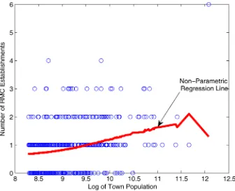
I designate the number of ready-mix concrete firms in a mar-ket asNjand the number of potential entrants in a market asNe. I set the number of potential entrants to six, the maximum num-ber of firms in any market in the data. I estimate the probability of entry using nonparametric regression,

ˆ ing parameterh=.43 to minimize the sum of squared errors from the regression. Figure 1 presents the number of ready-mix concrete establishments in a town plotted against town popula-tion, along with a nonparametric regression of this relationship whereNˆ(xi)=NePˆ(xi).

1.2 Estimator

I use a entry model similar to that discussed by Aradillas-Lopez and Tamer. Firms are ex ante identical but receive dif-ferent private information shocks to the profits that they will receive on entry. I parameterize a firm’s profits as

πi=β xi

whereβ measures the effect of population on profits andαis the effect of an additional competitor on profits. Initially, the highest prior that I can assign to the entry probability of my op-ponents is that all opop-ponents enter, that is,¯e(xi)0=1. Likewise, the lowest possible prior that I can have is that no other firms en-ter the market, that is,e(xi)0=0. Given these upper and lower bounds on beliefs, a firm chooses to enter if it makes positive profits. Aradillas-Lopez and Tamer define level-krationality or level-krationalizability as behavior that can be rationalized by some beliefs that survive at leastk−1 steps of iterated deletion of dominated strategies. Thus the first stage of this process of iterated deletion of dominated strategies assigns possible entry probabilities at 0 and 1. Bounds on a firm’s expected profitsπ_ik (where kdenotes the level-kof rationality) given the assump-tion that effect of addiassump-tional firms is to decrease profits are

xiβ+αNee¯(xi)0+ǫi≤πi0≤xiβ+αNee(xi)0+ǫi. The bounds on the probability that a firm will enter given

K=0, denoted asei(θ ), follow directly,

Fǫ(xiβ+αNee¯(xi)0)≤ei(θ )≤Fǫ(xiβ+αNee(xi)0), whereFǫis the cdf ofǫ.

From here, it is straightforward to iterate on the upper and lower bounds for entry probabilities for levels of rationality greater than K=0. This process of iteration is equivalent to deleting dominated strategies. The upper bound on the entry probability for a firm is denoted bye¯(xi)k, and the lower bound In my application I just assume that ǫhas a standard normal distribution, that is,ǫ∼N(0,1).

Aradillas-Lopez and Tamer define the identified set for

level-krationality as the set of parameter values that satisfy the

level-k′ conditional moment inequalities for each k≥k′ ≥1 with

(3)

Figure 1. Entry patterns of ready-mix concrete plants in isolated markets.

probability 1. Thus a natural estimator for this model can be derived from looking for cases when the entry probabilities in the data are outside of the upper and lower bounds. The crite-rion for one such estimator is

Qk(θ )= i

[ ˆP(xi)− ¯ek(θ ,xi)]+2+[ek(θ ,xi)− ˆP(xi)]+2. (4) The identified set is just the set of parameters θ for which there are no violations of the upper and lower bounds,

ˆ

I= {θ∈:Qk(θ )=0}. (5)

In contrast, the standard estimator using a symmetric NE, such as the model of Seim (2005), would look for an entry prob-abilitye∗that is a fixed point to the best-response mapping, that is,e∗such that

e∗=Fǫ(xiβ+αNee∗).

This would lead to an estimator with the following criterion function, the distance between the symmetric Nash solution and the data:

QN(θ )= i

[ ˆP(xi)−e∗(θ ,xi)]2. (6)

Note that the estimator that minimizes the Nash criterion in equation (6) generally will be point-identified. The estimated parameter for the Nash criterion is θˆN=argminθQN(θ ), the

(generically) unique parameter that minimizes the deviations of the Nash prediction from the data.

Figure 2 presents the prediction of both the rationalizable model for up to 100 levels of iterated deletion of dominated strategies and the NE model for parameters α = −.42 and β =.1. The top lines show the upper bound on the number

of firms that enter, corresponding to the smallest possible be-lief about the number of other firms that might enter. Like-wise, the bottom lines correspond to the lower bound on the number of expected entrants if I held the greatest belief about the entry probability of opponents. The middle dashed line shows the prediction from the symmetric Nash model. Note that whereas the upper and lower bounds grow closer to each other as we increase thek-level of iterated deletion of strate-gies, they do not necessarily converge to the symmetric Nash model. Indeed, it is possible to sustain asymmetric equilibria in this model of the type 1, firms enter because they expect other firms not to enter, and 2, firms stay out of the market because they expect other firms to enter. The larger the competitive in-teraction parameter α, the larger the split between the upper and lower bounds. In fact, it is this effect of competitive in-teractionαon the spread between the upper and lower bounds that makes it difficult to reject very highly competitive interac-tions.

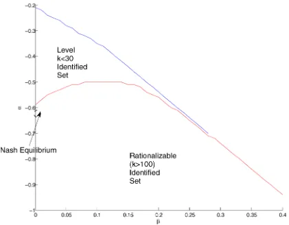
Figure 3 presents the identified set described by (5) for the model of Aradillas-Lopez and Tamer using ready-mix concrete data where I letkgo from 0 to 100. Askincreases above 30, the blue shaded area in the top left disappears from the identi-fied set, indicating that assuming a higher level-kof rationality shrinks the identified set. In particular, the highest possibleα in the identified set decreases from−.2 to−.5 askgoes from 0 to about 30. Abovek=30, the identified set stays about the same, as would be expected given that in a finite number of iterated deletion of dominated strategies gives the set of ratio-nalizable strategies. The upper bound on the effect of competi-tion on profits is aboutα= −.50, so we can state conclusively that there is an effect of competition on profits in the ready-mix concrete industry. But there is no lower bound on the effect of competition on profits, so we cannot reject the assertion that

(4)

Figure 2. Model predictions forklevels of iterated deletion of dominated strategies and NE (α= −.42 andβ=.1).

Figure 3. Identified set for the model of Aradillas-Lopez and Tamer using ready-mix concrete data [α,βsuch thatQ(α, β)=0].

(5)

competition reduces profits by an arbitrarily large amount. To understand this result, it is worth remembering the increasing the effect of competition on profits pushes out the upper and lower bounds in Figure 2, because a large effect of competition on profits makes it possible to sustain asymmetric equilibria of the type where if I expect no other firm to enter, then I will enter for sure, and if I expect other firms to enter, then I will choose not to enter myself. Thus increasing the competitive pa-rameterα will enlarge the set of permissible entry probabili-ties, which makes it impossible to form a lower bound on α. This seems to be a fairly generic result that casts some doubt on estimates from the entry literature on the strength of com-petition. Figure 3 also shows the location of the parameter that minimizes the Nash criterion function presented in (6). Note that this parameter gives no information on the size of the iden-tified set.

2. DYNAMICS, LEARNING, AND STATIC MODELS

In the previous section I gave a sketch of an empirical im-plementation of the ideas of Aradillas-Lopez and Tamer. In this section I take a step back and discuss how closely the model that Aradillas-Lopez and Tamer propose matches common ap-plications in empirical industrial organization.

2.1 Dynamic Oligopoly and Two-Period Models

The main gap between the model of Aradillas-Lopez and Tamer and the most recent work studying entry (e.g., Ryan 2006; Sweeting 2007; Collard-Wexler 2006) is the use of a two-period or static model instead of an explicitly dynamic model. In a two-period model, firms first make their entry de-cision and then receive a continuation value given the actions of other firms. These models were first used by Bresnahan and Reiss (1991) and Berry (1992) to study entry into dental and air-line markets. Two-period models can be considered a “reduced-form” for a fully dynamic model, because airlines or dentists enter at different times and have the option to exit and reen-ter in the future. There are also a limited number of situations in which a simultaneous entry game corresponds exactly to the application in mind. I will discuss one particular example in the next section.

Using a static model to estimate behavior that is the out-come of a dynamic entry process may lead us to misunder-stand the importance of multiple rationalizable strategies. For instance, much of the uncertainty in a static model come from the fact that either I do not know what my opponents will do or there are many possible actions that my opponents can take that are rationalizable. But in a dynamic context, this problem should be mitigated substantially, because entry and exit rates in most industries tend to be fairly low; for instance, in the ready-mix concrete industry, there is a 5% probability that a firm will enter or exit over the next year, and the probability of two firms entering simultaneously is<1%. Given how low these entry and exit rates are, it is not clear how big a differ-ence in expected payoffs that I would expect if I were using the most pessimistic or the most optimistic belief about the en-try probabilities of my rivals. Moreover, given the high sunk costs in many industries, why not wait for other firms to en-ter before deciding to exit the market? Note that there are still

multiple rationalizable strategies in dynamic games, but this is not the same problem as multiplicity in the static reduced form.

2.2 Learning and Nash

NE is frequently justified as the outcome from a learning process (see, e.g., Fudenberg and Levine 1998). In cases where agents have extensive experience with a market, NE can be jus-tified as the outcome of a learning process. Thus rationalize-ability seems to be too weak.

Alternatively, Nash can be conceived as a best response to the historical distribution of strategies used by firms. Suppose that I am a construction firm trying to bid in a first-price auction to build a highway. I might try to use introspection about the strategies of other players to form my beliefs about what other firms will bid. Alternatively, I could just review similar auctions to get an idea of the distribution of the bids of my opponents. In the context of entry into the ready-mix concrete industry, I could simply estimate the entry policies of my rivalseˆ(xi)in similar markets. I could then use these estimated probabilities to compute my expected value should I choose to enter.

Aradillas-Lopez and Tamer’s model is an exact fit in a lim-ited set of empirical applications. First, we need to look for sit-uations in which firms enter at the same time. Second, an ideal application is to an industry where there is little experience of entry, which would allow firms to simply look at the distribution of the strategies of their opponents. Perhaps, the best example of this is the study of Augereau, Greenstein, and Rysman (2005) of the adoption of one of two types of 56-K modem technology by Internet service providers (ISPs). Between May and June 1997, ISPs had to choose one of two incompatible 56-K mo-dem technologies. Choosing the same technology as rival ISPs lowered profits. This is clearly a one-shot game, because revers-ing the modem choice was expensive and there was no previous experience with the technology on which to draw to try to un-derstand what opponents would do. Goldfarb and Yang (2007) extended the work Augereau, Greenstein, and Rysman (2005) by looking at weakening the Nash assumption in the 56-K mo-dem adoption decision. They estimated the model of Camerer, Ho, and Chong (2004), which assumes that agents are playing against a Poisson distribution of level-ktypes. They found ev-idence that managers use limited introspection into the actions of their rivals, and that the degree of introspection is positively correlated with the education level within the market.

3. CONCLUSION

Aradillas-Lopez and Tamer have written a provocative article that challenges applied researchers in industrial organization to rethink the behavior that we use in empirical work. In particular, the assumption that agents are playing Nash can be quite strong in situations where there is limited experience with a market. Moreover, in many cases Nash is more than we need to esti-mate parameters. As I hope that this empirical implementation has demonstrated, I believe that Aradillas-Lopez and Tamer’s approach will be adopted in empirical work.

(6)

ADDITIONAL REFERENCES

Augereau, A., Greenstein, S., and Rysman, M. (2005), “Coordination versus Differentiation in a Standards War: The Adoption of 56K Modems,”RAND Journal of Economics, 37, 887–909.

Berry, S. T. (1992), “Estimation of a Model of Entry in the Airline Industry,” Econometrica, 60, 29.

Camerer, C. F., Ho, T.-H., and Chong, K. (2004), “A Cognitive Hierarchy Model of Behavior in Games,”Quarterly Journal of Economics, 19, 861. Collard-Wexler, A. (2006), “Demand Fluctuations and Plant Turnover in the

Ready-Mix Concrete Industry,” working paper, New York University, Stern School of Business, Economics Department.

Fudenberg, D., and Levine, D. (1998),The Theory of Learning in Games, Cam-bridge, MA: MIT Press.

Goldfarb, A., and Yang, B. (2007), “Are All Managers Created Equal?” working paper, University of Toronto, Marketing Department.

Ryan, S. P. (2006), “The Costs of Environmental Regulation in a Concentrated Industry,” working paper, Massachusetts Institute of Technology, Economics Department.

Seim, K. (2005), “An Empirical Model of Firm Entry With Endogenous Product-Type Choices,”Rand Journal of Economics, 37, 619–640. Sweeting, A. T. (2007), “The Costs of Product Repositioning: The Case of

For-mat Switching in the Commercial Radio Industry,” working paper, Duke Uni-versity, Economics Department.

Rejoinder

Andres A

RADILLAS

-L

OPEZ

Department of Economics, Princeton University, Princeton, NJ 08544

Elie T

AMER

Department of Economics, Northwestern University, Evanston, IL 60208 (tamer@northwestern.edu)

We wish to thank all of the discussants for their thoughtful and interesting comments. We would like to take this opportu-nity to briefly address some of the issues raised implicitly and explicitly in their comments. In doing so, we would like to clas-sify these comments into two broad categories:implementation

andextensions.

1. IMPLEMENTATION

The aim of the article was to provide identification results under rationalizable behavior, leaving for future and ongoing research the problem of estimation and inference using these identification results. A number of comments were aimed at the issue of implementation and usefulness of these results for practitioners in more complicated game-theoretic settings than those studied in the article. We begin with the question of com-putational issues.

1.1 General Issues for Applied Researchers

One of the potential advantages of our approach is the ability to bypass the need to compute the equilibria in the game. But our article provided no insight into the actual computational complexity of doing inference based on rationalizable behav-ior. This was addressed through a nice example by Collard-Wexler, who estimated a static model of entry in the ready to mix cement industry using level-krationality and compared those with estimates obtained assuming Nash. It turns out that with Nash, the model point identifies the parameter vector of interest, whereas with rationalizability, even as k→ ∞, the model puts one-sided bounds on the parameters. This is not surprising and in fact demonstrates the power of Nash in sim-ple empirical setups where there is no heterogeneity. We also agree with Collard-Wexler’s point that in some entry settings, static games of incomplete information might not be the pre-ferred framework as a model and that a model with dynam-ics can be a better approximation. His comment also highlights

the need to incorporate correlation in unobservables into the method. As we mention in the article, our constructive iden-tification results can be extended to such cases, then the joint distribution of unobservables is assumed known, possibly up to a finite-dimensional parameter. Conceptually, our setup allows for correlation among the unobservables.

The need to develop a computational methodology based on rationalizable bounds that deals more realistically with unob-served heterogeneity was also addressed by Bajari. He correctly points out that a positive relationship between the actions of two agents could be the result of correlation across agents’ un-observed heterogeneity instead of a strategic interaction effect. As we point out in the article, at least in cases where normal-form payoffs have a simple structure, we retain the ability to partially disentangle unobserved beliefs from unobserved het-erogeneity and even would be able to deal with the case where beliefs are conditioned on unobservables as long as the joint distribution of these unobservables is assumed known. Work on cases where this distribution is unknown, although conceptually straightforward, is left for future research.

Bajari also suggests the need for an empirical application in which issues of rationalizability versus equilibrium can be ex-amined. This is reasonable because identifying power of equi-librium is ultimately an empirical question. Bajari then ques-tions the use of entry games as a basis for our model. Although it is true that a firm’s decision to enter a market is dynamic in nature, static entry models can be used as models to shed light on long-term market structure. In addition, our framework for studying identification under rationality as we define it still can be used to study static games other than entry. It also is certainly possible to generalize the current setup to handle a large set of