Full Terms & Conditions of access and use can be found at
http://www.tandfonline.com/action/journalInformation?journalCode=ubes20
Download by: [Universitas Maritim Raja Ali Haji] Date: 12 January 2016, At: 23:13
Journal of Business & Economic Statistics
ISSN: 0735-0015 (Print) 1537-2707 (Online) Journal homepage: http://www.tandfonline.com/loi/ubes20
Does Wealth Explain Black–White Differences in
Early Employment Careers?
Sílvio Rendon
To cite this article: Sílvio Rendon (2007) Does Wealth Explain Black–White Differences in Early Employment Careers?, Journal of Business & Economic Statistics, 25:4, 484-500, DOI: 10.1198/073500107000000124
To link to this article: http://dx.doi.org/10.1198/073500107000000124
Published online: 01 Jan 2012.
Submit your article to this journal
Article views: 52
Does Wealth Explain Black–White Differences
in Early Employment Careers?
Sílvio R
ENDONCentro de Investigación Económica—Instituto Tecnológico Autónomo de México (ITAM), Mexico D.F. 10700, Mexico (srendon@itam.mx)
In this article I inquire about the effects initial wealth has on black–white differences in early employment careers. I set up a dynamic model in which individuals simultaneously search for a job and accumu-late wealth, and fit it to data from the National Longitudinal Survey (1979-cohort). Regime changes and decompositions of racial differences reveal that differences in the labor market environment and in pref-erences account fully for racial gaps in wealth and in wages persisting several years after high school graduation. Differences in initial wealth partially explain differences in early employment careers.
KEY WORDS: Borrowing constraints; Consumption; Estimation of dynamic structural models; Job search; Racial differences; Unemployment.
1. INTRODUCTION
The last decade has witnessed a growing interest in the black–white wealth gap. Whereas historically income dispar-ity between blacks and whites has narrowed down (Smith and Welch 1989), wealth disparity remains large. Thus, whereas blacks earn between 50% and 64% of whites’ income, blacks’ wealth is only between 12% and 20% of whites’ wealth (Blau and Graham 1990; Wolff 1994; Menchik and Jianakoplos 1997; Oliver and Shapiro 1997; Scholz and Levine 2003). Recent studies have focused on the role of differences in income, ed-ucation, and patterns of marriage and fertility to explain racial gaps in wealth levels and growth rates (Gittleman and Wolff 2004; Altonji and Doraszelski 2005). I, on the other hand, examine whether causality may be also working in the op-posite direction, that is, whether initial wealth disparity ex-plains black–white differences in employed wages and em-ployment rates for high school graduates. Therefore, through-out this article I report differences in wages (the income of the employed) and in the unemployment rate rather than to-tal differences in income, as in other studies. To abstract from wage differences caused by skill gaps (Neal and Johnson 1996; Neal 2005), I restrict the analysis to individuals with the same level of schooling. Subsequently, I estimate a dynamic model of wealth accumulation and job search and find that initial wealth has essentially no influence in explaining racial disparities sev-eral years after high school graduation in comparison with labor market variables. Initial wealth only accounts for the racial gap in wealth and wages at thebeginning of employment careers. By contrast, differences in the labor market environment and in preferences are shown to account fully for both racial gaps, in wealth and in wages, persisting several years after high school graduation.
Imperfect capital markets allow wealth to affect job search outcomes: wealthier agents can search longer and obtain higher wages. This effect is formalized in a utility-maximizing job search model where agents’ reservation wages depend posi-tively on their wealth levels. Thus, wealth accumulation be-comes part of the optimal job search strategy in which un-employed agents run down their wealth to maintain consump-tion levels, and employed agents accumulate wealth to hedge against future unemployment spells, which also allows them to move to better paying jobs.
Utility-maximizing job search models are based on the sem-inal work of Danforth (1979), who analyzed in detail the role of wealth on an individual’s optimal job search strategy. In his framework, only the unemployed look for a job and receive wage offers from a nondegenerate distribution; the employed do not search and do not become unemployed and there is no de-cision about search intensity. In recent years several empirical studies have attempted to test utility-maximizing search models inspired by Danforth’s basic framework. In this article I gen-eralize Danforth’s model to allow for on-the-job search, wage growth, variations of arrival and layoff rates as a function of age, retirement age, and a parametric limit on borrowing. In par-ticular, I assume a parametric initial wealth distribution and un-observed heterogeneity with different types of individuals who differ in their labor market environments, initial wealth dis-tributions, borrowing constraints, and preferences. These fea-tures allow my model to generate predicted life-cycle trajecto-ries and distributions of employment status, wealth, and wages that match the observed ones.
The behavioral parameters of the model are recovered using the method surveyed by Rust (1988) and Eckstein and Wolpin (1989). I use the numerical solution to the joint job search and consumption problem to construct a distance function between the observed and the predicted paths of wealth, wages, and em-ployment transitions, which is minimized over the behavioral parameters. This approach has been used by Wolpin (1992), Eckstein and Wolpin (1999), Keane and Wolpin (2000), and Bowlus and Eckstein (2002) to study black–white labor mar-ket differences and to conduct policy experiments. I study the effects on wealth accumulation and labor market outcomes of regime changes consisting of assigning blacks the labor market conditions, initial wealth distribution and access to credit, and preferences of whites. Furthermore, I use these counterfactual experiments to perform a decomposition of the total race differ-entials into these three components.
A regime change that gives blacks the labor market condi-tions of whites is able to generate full convergence in labor mar-ket outcomes both in the short and in the long run. If, addition-ally, there is a switch in taste parameters, this regime change
© 2007 American Statistical Association Journal of Business & Economic Statistics October 2007, Vol. 25, No. 4 DOI 10.1198/073500107000000124
484
can also eliminate long-run wealth disparity, although not the initial wealth gap. On the contrary, a shift in initial wealth and access to credit fails to substantially narrow down the long-run racial wealth and wage gaps, but it is the only regime change that accomplishes the elimination of racial gaps in wealth and wages at the beginning of employment careers.
The remainder of the article is organized as follows. The next section explains the data source, the National Longitudinal Sur-vey of Labor Market Experience—Youth Cohort (NLSY), the selection of the sample, and the descriptive statistics; Section 3 describes the theoretical model; Section 4 explains the simu-lated method of moments estimation procedure; Section 5 an-alyzes the estimation results; Section 6 assesses, both formally and graphically, the performance of the model in replicating the main trends of the data; and Section 7 presents regime changes and decomposition of race differences based on the estimated parameters of the model. The main conclusions of the article are summarized in Section 8.
2. DATA
The National Longitudinal Survey of Labor Market Expe-rience—Youth Cohort (NLSY) contains data on household composition, military experience, school enrollment, and a week-by-week account of employment status, hourly wages, hours worked, and employers. An individual’s complete weekly work history can be constructed from 1978 until 1993. Respon-dents whose employment histories started before 1978, that is, those born before 1961, and for whom it is impossible to con-struct a complete employment history, are dropped from the sample. The final sample contains 158 black and 212 white high school male graduates born after December 31, 1960, who nei-ther went to college nor had any type of military experience. Black males were selected from the core and from the supple-mental sample, whereas white males were taken from the core sample. Wolpin (1992) and Rendon (2006) also used this se-lection of individuals whose behavior is well described by a search-theoretic framework that excludes the decision to join the military.
Given that blacks exhibit higher high school dropout rates and whites are more likely to continue studying after high school, it is possible that this sample selection leads to an under-estimation of the differences in labor market outcomes by race. As pointed out by Heckman, Lyons, and Todd (2000), the defin-ition of the sample is crucial in making inferences about black– white differentials. In this article the lower tail of the income distribution of blacks and the upper tail of the income distribu-tion of whites could be underrepresented. In spite of this, it will be shown that, under the assumption of exogeneity of educa-tional attainment, wage and wealth differences by race remain important.
To make the estimation tractable I aggregate the data into quarters. Each individual’s reported last week of school enroll-ment is assigned to its corresponding calendar quarter; employ-ment history starts in the quarter thereafter. An individual is em-ployed if he works 20 or more hours during the first week of the quarter; any other job held during the quarter is ignored. Oth-erwise, he is recorded as unemployed for that quarter. Reasons
for leaving a given employer are classed as layoffs or quits. In-dividuals returning to work for their old employers are recorded as having new jobs. The quarterly wage is the wage of the first week of the quarter in 1985 dollars times 13. The Consumer Price Index is used to deflate nominal values into real amounts. I evaluate the magnitude or potential for aggregation bias induced by the aggregation of data into quarters by compar-ing quarterly transitions computed uscompar-ing the observation of the first week with quarterly transitions implied by the weekly data for all black and white individuals in the survey. For both race groups aggregation tends to overestimate the persistence of un-employment and underestimate job loss. For blacks there is a slight overestimation of persistence of work for the same em-ployer, whereas for whites there is a slight underestimation of persistence of work for the same employer. This exercise reveals that the quarterly transitions are not that inaccurate, given the substantial omission of weekly observations. I re-port this exercise in Appendix A2, which, together with Ap-pendixes A3–A9, is contained in a separate document and is available from the author upon request.
Annual data on the market value of wealth are only avail-able for years 1985 until 1993, with the exception of year 1991; this information is assigned to the calendar quarter in which the interview took place, leaving all other quarters blank.
Wealth consists of financial assets, vehicles, and other as-sets (such as jewelry or furniture), all net of debts and all com-puted at their “market value,” defined by the NLSY as the amount the respondent would reasonably expect someone to pay if the particular asset were sold in its current condition at any point in time. Other less liquid types of wealth, such as residential property and business assets, are excluded as I as-sume that agents will only use the most liquid wealth to finance their job search. Jianakoplos, Menchik, and Irvine (1989), Blau and Graham (1990), and Smith (1995) showed that, as indi-viduals of both race groups become wealthier, they increase the proportion of their wealth in the form of residential prop-erty, business, farms, or other propprop-erty, and decrease the pro-portion of their wealth in the form of vehicles. Notably, at the same wealth level blacks systematically have a lower percent-age of their wealth in business property than whites, denot-ing a relative absence of black-owned businesses (Fairlie 1999; Fairlie and Meyer 2000). Thus, racial inequality in terms of the most liquid wealth will be lower than racial inequality mea-sured with total wealth. In Rendon (2006) I estimated a similar version of this model for one race group usingtotalwealth; ac-cordingly, as we will see in Section 5, in that article borrowing constraints are estimated to be tighter and the coefficient of risk aversion higher than in the current article.
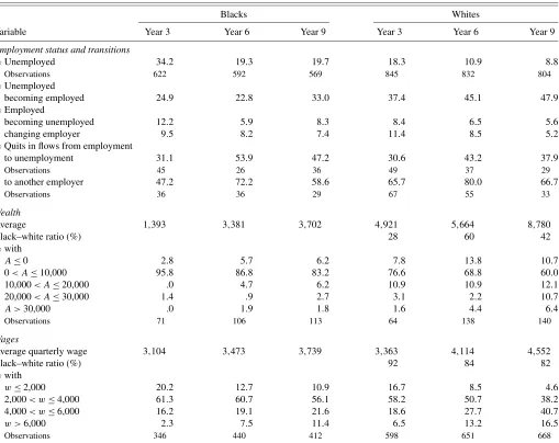
Table 1 shows the evolution of employment rates and tran-sitions, wealth, and wages 3, 6, and 9 years after high school graduation. From year 3 to year 9, the fraction of blacks who are unemployed decreases from 34% to 20%, while the cor-responding percentage for whites decreases from 18% to 9%. In the same period, blacks increase their wealth from $1,393 to $3,702, whereas whites increase their wealth from $4,921 to $8,780, that is, the black–white ratio of average wealth in-creases from 28% to 42%. The percentage of individuals with more than $10,000 increases from 1% to 11% for blacks, and from 15% to 29% for whites. Average wage, income of the em-ployed, for blacks increases from $3,104 to $3,739 and from
Table 1. Unemployment, wealth, and wages by number of years since graduation for black and white male high school graduates (amounts in 1985 dollars)
Blacks Whites
Variable Year 3 Year 6 Year 9 Year 3 Year 6 Year 9
Employment status and transitions
% Unemployed 34.2 19.3 19.7 18.3 10.9 8.8
Observations 622 592 569 845 832 804
% Unemployed
becoming employed 24.9 22.8 33.0 37.4 45.1 47.9 % Employed
becoming unemployed 12.2 5.9 8.3 8.4 6.5 5.6 changing employer 9.5 8.2 7.4 11.4 8.5 5.2 % Quits in flows from employment
to unemployment 31.1 53.9 47.2 30.6 43.2 37.9
Observations 45 26 36 49 37 29
to another employer 47.2 72.2 58.6 65.7 80.0 66.7
Observations 36 36 29 67 55 33
Wealth
Average 1,393 3,381 3,702 4,921 5,664 8,780
Black–white ratio (%) 28 60 42
% with
A≤0 2.8 5.7 6.2 7.8 13.8 10.7
0< A≤10,000 95.8 86.8 83.2 76.6 68.8 60.0 10,000< A≤20,000 .0 4.7 6.2 10.9 10.9 12.1 20,000< A≤30,000 1.4 .9 2.7 3.1 2.2 10.7
A >30,000 .0 1.9 1.8 1.6 4.4 6.4
Observations 71 106 113 64 138 140
Wages
Average quarterly wage 3,104 3,473 3,739 3,363 4,114 4,552
Black–white ratio (%) 92 84 82
% with
w≤2,000 20.2 12.7 10.9 16.7 8.5 4.6 2,000< w≤4,000 61.3 60.7 56.1 58.2 50.7 38.2 4,000< w≤6,000 16.2 19.1 21.6 18.6 27.7 40.7
w >6,000 2.3 7.5 11.4 6.5 13.2 16.5
Observations 346 440 412 598 651 668
NOTE: Wages are only the labor income of the employed and do not include any income of the unemployed. Number of observations are noted in smaller font.
$3,363 to $4,552 for whites, meaning that the black–white ra-tio of average wage decreases from 92% to 82%. It is clear that wealth accumulation does accompany the increase in employ-ment rates and wages that occurs after graduation from high school, and that a reduction in the racial wealth gap is associ-ated with a widening of the racial wage gap.
Table 2 reports average wealth by wage level, number of years since graduation, and race group. Wages measure the quarterly income of the employed only; the unemployed are not included in this table. It is shown that agents with higher wages tend to have a higher level of wealth. No more than 6 years after graduation, blacks with wages below $2,000 have an av-erage wealth of $724, whereas blacks with wages above $6,000 have an average wealth of $5,634. The corresponding wealth of whites for the same wage brackets is, respectively, $1,396 and $8,511. These descriptive statistics show the existence of a link between labor market progress and wealth accumulation for both race groups.
Table 3 relates saving behavior to employment transitions be-tween two periods for which wealth data are available. As the
interviews were conducted in different quarters for different in-dividuals, this time interval does not necessarily correspond to four quarters. For both race groups, becoming or staying un-employed is associated with wealth decumulation, whereas
be-Table 2. Average wealth by wages and years after graduation (in 1985 dollars)
Blacks Whites Wages Years≤6 Years>6 Years≤6 Years>6
w≤2,000 724 1,674 1,396 2,338
38 38 48 27
2,000< w≤4,000 1,762 2,361 4,056 6,049
177 202 193 208
4,000< w≤6,000 4,528 6,108 6,227 8,747
53 76 94 168
w >6,000 5,634 9,377 8,511 11,283
7 30 34 52
NOTE: This table only contains observations for employed individuals. Wages are only labor income. Number of observations are noted in smaller font.
Table 3. Average quarterly savings by employment transitions: blacks’ savings/whites’ savings
t+
Employment Un- Same New
statust employment employment employment Total Unemployment −101/−2,918 1,720/365 766/−738
123/41 109/81 568/122
Employment −953/−1,514 −73/545 243/129 −141/329
98/68 483/698 150/194 731/960
Total −484/−2,043 −95/561 870/206 77/209
221/109 483/698 259/275 963/1,082
NOTE: Wealth is only observed annually, at quartertand quartert+. Employment transitions and savings are, respectively, the employment and the average quarterly wealth variation between these two quarters. The ratio of number of blacks to the number of whites is noted in smaller font.
coming employed or changing employer is associated with in-creases in wealth. Staying with the same employer is associated with wealth accumulation for whites, and with wealth decumu-lation for blacks. Black individuals who are unemployed and become employed save on average $1,740 between two quar-ters; the corresponding amount for whites is $365. White indi-viduals who are employed and become unemployed decrease their wealth by $1,515; the corresponding amount for blacks is $953. Explaining these related trends requires a theoretical model that will account jointly for wealth accumulation and employment transitions.
3. MODEL
In this section I describe a model of wealth accumulation and job search under borrowing constraints. It is an extension of Danforth’s (1979) model to allow for on-the-job search, wage growth, variations in arrival and layoff rates as a function of age, retirement age, and a parametric borrowing limit.
An individual maximizes expected utility of consumption over his life,TF(=262)quarters. He can be employed or
un-employed during his active life,T (=162)quarters, after which he retires and lives off his savings. Each period he faces a utility functionU (·)over consumption and, when employed, he suf-fers a constant utility loss captured byψ≥0, which represents the disutility of working.
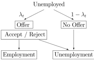
While unemployed at period t he receives, with probabil-ity λt, one wage offer x drawn from the known base wage
offer distributionF (·),x∈(w, w), 0< w < w <∞. An un-employed individual becomes un-employed if he receives and ac-cepts a wage offer; otherwise he remains unemployed. Transi-tions from unemployment are illustrated in Figure 1.
While employed at periodt, an individual can be laid off with probabilityθt and receive a new wage offer with probabilityπt,
drawn from the same base distributionF (·). If he is not laid off and receives a job offer, he can accept it and switch to a new job, reject it and stay in the current job, or reject it and quit to unemployment. If he is not laid off and does not receive a job offer, he has to decide between staying in his current job or quitting to unemployment. If he is laid off, he can still receive a job offer; accepting it means switching to a new job; rejecting it means becoming unemployed. If a person is laid off and does
Figure 1. Transitions from unemployment.
not receive an offer, his only option is to become unemployed. The possible transitions from being employed are shown in Fig-ure 2.
When unemployed, the agent receives transfersb, which are nonlabor income such as family transfers and unemployment compensation net of search costs. When employed, the agent experiences wage growth as a function of age, that is, his cur-rent wage wt depends on the initial wage draw ω and aget.
Similarly, both the probability of receiving an offer while un-employed and while un-employed,λt andπt, respectively, as well
as the layoff rate θt, depend on the agent’s age t. Modeling
wage and arrival rates as functions of experience would have been preferable, but would also increase drastically the compu-tation burden to solve and estimate this model.
At each period t, given his employment state and his wealthAt, the agent determines his consumption Ctu andCte,
and thereby his wealth for the next periodAut+1andAet+1. Ini-tial wealth is inherited and final wealth is zero. The rate of returnris constant; the subjective discount factor isβ∈(0,1). Agents can save freely, but borrowing is restricted so that cur-rent wealth cannot be lower than an age-dependent levelBt. In
a free capital market with fully risk-averse lenders, individuals can borrow up to the level they can pay back with certainty, that is, the “natural borrowing limit” (Ljungqvist and Sargent 2000), which is the present discounted value of the lowest possible income level b:Bt = −Tτ=tb/(1+r)T
−τ. Wealth
levels below this limit imply nonpositive consumption, C =
Bt +b−Bt+1/(1+r)=0, which is not admissible for utility
functions that satisfy the Inada condition limC→0U (C)= ∞.
Hence, the only nonredundant constraint isBt>Bt, which
al-lows us to express and parameterize the borrowing constraint as a fraction of the natural constraint. Letsmeasure the tightness of the borrowing constraint as a fraction ofBt; then the lower
bound on wealth isBt=sBt,s∈ [0,1].
The expected lifetime utility of a retired agent of aget,VtR, depends on wealthAt:
whereATF+1=0. This agent saves voluntarily for retirement
with full control over his pension funds, so that the dynamic problem becomes “a cake-eating problem.” A possible exten-sion of this model is to allow for a penexten-sion system with realistic contribution schemes during the working lifetime and pensions during retirement with an increasing mortality. However, since the estimation will only contain a young labor force, this ex-tension should not affect the main results substantially. Accord-ingly, it is left for future research.
Figure 2. Transitions from employment.
When unemployed, expected lifetime utility at aget,Vtu, de-pends on wealthAt:
Vtu(At)
= max
Au t+1≥Bt+1
U
At+b− Aut+1 1+r
+β
λt+1 max[Vte+1(Aut+1, x), Vtu+1(Aut+1)]dF (x)
+(1−λt+1)Vtu+1(Aut+1)
.
When employed, expected lifetime utility at aget,Vte, de-pends on wealthAt and wagew:
Vte(At, ω)= max Ae
t+1≥Bt+1
U
At+wt(ω)− Aet+1 1+r
−ψ
+β
(1−θt+1)
πt+1 max[Vte+1(Aet+1, x),
Vte+1(Aet+1, ω), Vtu+1(Aet+1)]dF (x)
+(1−πt+1)max[Vte+1(Aet+1, ω), Vtu+1(Aet+1)]
+θt+1
πt+1 max[Vte+1(A e t+1, x),
Vtu+1(Aet+1)]dF (x)
+(1−πt+1)Vtu+1(Aet+1)
.
This dynamic programming (DP) problem has a finite hori-zonT and a “salvage value” that is the present discounted util-ity at retirement age, that is, att=T +1:Vtu(At)=VtR(At),
and Vte(At, ω)=VtR(At). The solution to this problem
in-cludes two policy rules for wealth accumulation, Aut+1(At)
and Aet+1(At, ω), and a reservation base wage ω∗t(At) =
{ω|Vtu(At)=Vte(At, ω)}. In this model, under certain
condi-tions nobody will work for a wage belowb, that is:
Proposition 1. Ifλt+1≥πt+1andψ≥0, thenwt(ω∗t(At))≥ b,t=1, . . . , T.
For the proof see Appendix.
Notice that requiring the arrival rate while unemployed to be higher than that while employed is a sufficient but not necessary condition for reservation wages to be greater or equal to unem-ployment transfers. Even if this condition is not fulfilled, high disutility levels associated to working can generate reservation wages that exceed unemployment transfers.
In the absence of analytical solutions for this problem, and to solve it numerically, one needs to assume specific functional forms:
1. a constant relative risk aversion (CRRA) utility function U (C)= C11−−γγ−1, where γ >0 is the coefficient of risk aversion that satisfies the Inada conditions
2. a truncated lognormal wage offer distribution lnω ∼
N(μ, σ2|lnω,lnω);
3. a wage growth functionwt(ω)=ωexp(α1t+α2t2)
4. age-dependent arrival and layoff rates given by the logis-tic function
qt=
q0exp(αqt )
1+q0[exp(αqt )−1]
whereq= {λ, π, θ},
andq0are the initial arrival and layoff rates. This
expres-sion comes fromqt=exp(αq0+αqt )/[1+exp(α0q+αqt )]
and lettingαq0=ln(q0/[1−q0]).
Then the model is solved recursively on a discretized state space. Using longer period lengths for the more distant future value functions in the DP problem makes the estimation more tractable (Wolpin 1992). Appendix A3 describes in detail the discretization and the numerical solution technique.
As shown in Rendon (2006), this model produces policy rules with the following features:
1. The unemployed decumulate wealth. That is, they main-tain their consumption while searching for a job by de-creasing their wealth monotonically until reaching the borrowing limit.
2. The employed can accumulate or decumulate wealth, de-pending on their wages and current wealth, so that wealth converges to some age-dependent desired level. They keep this wealth as a precaution to cushion future unem-ployment spells that may follow, if the layoff rate is not zero. As retirement age approaches, they increase their wealth accumulation.
3. The reservation wage is increasing in wealth. This means that wealthier agents are more selective and end up with higher accepted wages.
These policy rules imply a close interaction between la-bor market turnover and saving decisions. During unemploy-ment spells, longer for wealthier people, reservation wages decline and hazard rates increase. In contrast, during employ-ment spells, and for some combinations of current wealth and wages, wealth and reservation wage increase. It may occur that the reservation wage exceeds the current wage, in which case the current job is no longer preferable to unemployment. Bar-ring a better wage offer from a new employer, the agent will quit his current job to search for a better one while unemployed with higher arrival rates. Thus, wealth accumulation underlies quits to unemployment, which reflect the agent’s permanent desire to move to better paying jobs.
As explained in Rendon (2006), quits to unemployment can only happen in this framework if arrival rates are higher while unemployed than while employed. Although this difference is not assumed in the model and is not a restriction imposed in the estimation, observed quits will yield estimated parameters that satisfy this difference. Notice that the incentive to quit is there in spite of age wage growth.
With these features, the policy rules will be able to generate realistic employment transitions and trajectories and distribu-tions of wealth and wages over the life cycle.
4. ESTIMATION
The estimation strategy is designed to recover the behavioral parameters of the theoretical model. I assume that individuals start off their careers with a wealth level drawn from a para-metric initial wealth distribution and, for each parameter set, I compute the policy rules that solve the DP problem and use them to generate simulated career paths. Then, at each iteration of the parameters I construct a measure of distance between the observed and the simulated moments, namely, the distribu-tions of employment status and transidistribu-tions, wages, and assets. The estimation is thus a simulated method of moments (SMM) procedure in which the parameter estimates of the theoretical model are the minimizers of this function.
All individuals start off their careers being unemployed, with a wealth level A0 drawn from a displaced lognormal
distrib-ution, ln(A0−B0)∼N(μ0, σ02). I add the lowest admissible
wealth levelB0to each unobservable initial value of wealth to
make the term inside the logarithm positive. The identification of the parameters of this function is not only given by wealth data, which are scarce for the first quarters after graduation, but also, in the presence of persistence in observed wealth values over time, by employment transitions and wages over time. The parameters to estimate are then the following:
1. labor market parameters: 1= {λ0, π0, θ0, μ, σ, α1, α2,
from the reservation wage rule by the observed transitions, ac-cepted wages, and wealth level at each quarter after graduation. The interest rater and the discount factorβ are not identified separately from the arrival rates, so they are fixed at .015 and .98, respectively. The other parameters, namely γ ands, are specific to a utility-maximizing job search model, which gener-ates rules for wealth accumulation, and are pinned down by the observed evolution of wealth by employment status and wages. Individuals do not differ only in their initial wealth, but also in other characteristics that have permanent effects on their work history. Assuming there is only one type of agent would, therefore, lead to making wrong inferences, in particular with regard to the estimation of wage offer distributions and arrival rates (Lazear 1979; Orazem 1987). To prevent this I introduce unobserved heterogeneity in the estimation and assume eight types of agents within each race group, which requires solving the DP problem eight times, one for each type of agent.
I assume two types for each of the three subsets of parame-ters, indexed by 1 and 2. Therefore, there are 8=23types of individuals characterized by each possible combination of the three subsets: ij k = {1i, 2j, 3k},i, j, k=1,2. The
proba-bilities of being Type 1 for each of the three subsets of para-meters are denoted as p1=Pr(11), p2=Pr(21), and p3=
Pr(31), so that the proportion for each type combination in the subsample ispij k,i, j, k=1,2, obtained as the product of the
probabilities of each type for each subset of parameters:
p111=p1p2p3,
Accordingly, the vector for all parameters of the model is de-fined as = {11, 21, 31, 21, 22, 32, p1, p2, p3} and
con-tains the two types of the three subsets of parameters and three type probabilities.
I generate simulated career paths for 8,000 individuals, that is, 1,000 draws for each type of agent in each subsample. The moments used in this estimation are the cell-by-cell probability masses for the following distributions:
1. wealth distribution (10 years×5 moments) 2. wage distribution (10 years×4 moments) 3. employment status (10 years×2 moments)
4. employment transitions from unemployment (10 years×
2 moments)
5. employment transitions from employment (10 years×3 moments)
6. layoffs from employment to unemployment (10 years×
2 moments)
7. layoffs when changing employer (10 years×2 moments) Thus, there are 200 moments to estimate 32 parameters, 16 for each type of agent plus 3 proportions of types for each race group. These simulated moments are computed for each year and without excluding actually missing observations (these mo-ments barely change when they are computed excluding simu-lated individual and quarterly observations when the observed counterpart is missing). The SMM procedure relates a parame-ter set to a weighted measure of distance between sample and simulated moments:
S()=m′W−1m,
wheremis the distance between each sample and simulated moment and W is a weighting matrix. As shown in Appen-dix A4, the matrixW can be chosen so that this weighted dis-tance equals the sum of theχ2-statistics of the selected distri-butions. In that case, minimizing this function is equivalent to minimizing a goodness-of-fit measure: m′W−1m=χ1302 . Hence, fit measured by this criterion is the best that can be attained. The estimated behavioral parameters are thus ∗=
arg minS().
The function is minimized using Powell’s method (Press, Teutolsky, Vetterling, and Flannery 1992), which requires only function evaluations, not derivatives. This algorithm first calcu-lates function values for the whole parameter space and then
searches for the optimal parameter direction in the next it-eration for function minimization. Underlying the computa-tion of this optimal direccomputa-tion there is an implicit model of the derivative structure of the objective function. Once a new set of parameters is obtained, the algorithm goes back to calcu-late a new function value ft, and the process is repeated
un-til a convergence criterion is satisfied, namely, that the per-centage variation of this value falls below a certain value: 2|ft −ft−1|/(|ft| + |ft−1|)≤10−10. Asymptotic standard
er-rors are calculated using the outer-product gradient estimator; their computation is explained in greater detail in Appendix A5.
5. ESTIMATION RESULTS
In this section I discuss the parameter estimates for the two race groups and compare graphically and numerically actual and fitted moments: hazard rates at the first unemployment spell, trajectories for all observed variables, and wealth varia-tions by employment transivaria-tions.
The parameter estimates by race and type and their corre-sponding asymptotic standard errors are reported in Table 4. The first set of parameters, which characterize the labor mar-ket environment, is reported in the upper part of the table. The probabilities of receiving an offer while unemployed are ini-tially lower but grow faster for blacks than for whites. In the first period out of school, these are 69% for Type 1 and 30% for Type 2 of blacks. However, 40 quarters after graduation they have grown substantially to 83% and 98%, respectively. For whites these probabilities are initially 84% for Type 1 and
Table 4. Parameter estimates and asymptotic standard errors (in small fonts) (r=.015,β=.98)
Blacks Whites
Type 1 Type 2 Type 1 Type 2 Parameter Est. ASE Est. ASE Est. ASE Est. ASE
1
Base unemp. arrival rate %: λ0 69.30 4.65 29.47 55.30 83.62 21.45 57.56 3.81
Base emp. arrival rate %: π0 16.53 .73 81.24 28.21 9.90 6.18 53.42 11.61
Base layoff rate %: θ0 22.31 3.13 16.83 14.02 7.22 .79 13.25 2.11
Mean base log-wage dbn: μ 7.19 .07 6.58 .11 6.91 .02 7.71 .02
St. dev. base log-wage dbn: σ .60 .05 .63 .05 .50 .01 .45 .03
Unemp. arrival rate growth×102: αλ 1.93 .50 11.84 42.04 7.58 2.33 1.09 .43
Emp. arrival rate growth×102: απ .40 .25 .17 .36 3.20 2.00 .16 .16
Layoff rate growth×102: αθ −6.01 .62 −1.72 2.53 −1.06 .41 −3.65 .63
Wage growth (linear)×103: α1 8.60 1.79 1.27 .64 9.04 .12 14.42 1.62
Wage growth (quadratic)×105: α2 −4.00 .78 −3.41 2.67 −1.70 .32 −24.15 2.20
Proportion of Type 1: p1 57.41 4.46 43.67 5.15
2
Borrowing tightness %: s .43 .04 2.27 .27 4.85 .42 4.66 2.31
Mean of log-wealth dbn: μ0 6.17 .00 10.46 .00 8.77 2.53 10.59 2.04
St. dev. of log-wealth dbn: σ0 .05 .33 1.52 .41 1.73 1.09 1.86 .98
Proportion of Type 1: p2 79.76 7.54 86.45 1.92
3
Unemployment transfers: b 1,049 73 312 237 515 41 326 209
Risk aversion γ 1.08 .00 .30 .19 1.07 .03 1.31 .09
Disutility of working: ψ .20 .06 .99 6.21 .11 .03 .20 .07
Proportion of Type 1: p3 63.66 2.86 90.65 .93
Criterion value: χ2 283.20 343.11
58% for Type 2; 40 quarters later they have not grown much: 99% and 68%, respectively.
On the other hand, the probability of receiving an offer while employed is higher for blacks than for whites: it is initially 17% for Type 1 and 81% for Type 2 of blacks and 10% for Type 1 and 53% for Type 2 of whites. For both race groups, these prob-abilities do not grow much with age: 40 quarters after gradua-tion they become 19% and 82% for blacks and 28% and 55% for whites. The relatively slow growth of offer rates while em-ployed in contrast to the fast growth of offer rates while un-employed, captures the observed trend of decreasing job-to-job transitions over time that is simultaneous to exit rates from unemployment remaining pretty constant. To match increasing reservation wages, a result of wealth accumulation, arrival rates while unemployed have to go up so that exit rates remain more or less constant. Thus, if agents are becoming more selective in their job acceptance decisions and are moving up to better paying jobs, because of changing employers and of age wage growth, matching observed decreasing job-to-job transitions re-quires offer rates while employed not to grow too fast.
Finally, the layoff rate is initially higher but decreases faster for blacks. Whereas it is 22% for Type 1 and 17% for Type 2 of blacks, it is 7% for Type 1 and 13% for Type 2 of whites. Forty quarters after graduation these parameters become, re-spectively, 3% and 9% for blacks and 5% and 3% for whites, which means that there is relatively fast convergence in layoff rates. Only for blacks of Type 2, these arrival and layoff rates, both the initial values and the associated variation parameters, exhibit large standard errors; for all other groups they are esti-mated precisely.
Blacks exhibit lower means but higher standard deviations of the log-wage offer distributions than whites. These parame-ters imply an estimated initial mean quarterly wage offer for Type 1 and Type 2 of $1,999 and $1,590 for blacks and $1,575 and $2,511 for whites, respectively. Wages grow at a declin-ing rate for both races, but they grow higher for whites, who also reach a maximum level later in their working life: at 266 and 30 quarters for Type 1 and Type 2, respectively, of whites. The equivalent for blacks is 108 and 19 quarters. The highest attainable mean wage offers are $3,173 for Type 1 and $1,609 for Type 2 of blacks, and $5,235 for Type 1 and $3,115 for Type 2 of whites. Thus, although wages of Type 1 are initially the lowest of whites, because of their higher growth, they end up overtaking wages of Type 2. Asymptotic standard errors for these parameters are in general small, with the exception of the quadratic term of wage growth for Type 2 of blacks, which is found to be nonsignificant.
Whereas these implications are useful in providing a first glance on the evolution of wage offers, they do not consider wealth-dependent labor turnover (agents switching jobs and employment states depending on their wealth position) and therefore do not imply that wages for a given individual will peak at the above age. Simulations of the model over the in-dividual’s life cycle yield quarterly wages that peak at $7,540 for blacks and $10,118 for whites. The interested reader will find further insights on the maximum attainable wages over an individual’s life cycle in Appendix A6.
These parameters are characteristic of the standard search model and represent a labor market environment that is more fa-vorable for whites than for blacks. As in Wolpin (1992), whites
have a better wage offer distribution and more wage growth. However, here the differences in arrival rates are much larger for both race groups: arrival rates while unemployed are higher, arrival rates while employed are lower, and layoff rates are higher. Accounting for the evolution of wealth and the reason for leaving the current employer, particularly voluntary quits from employment to unemployment, require larger differences between arrival rates by employment status and larger layoff rates.
The second set of parameters is specific to a utility-maxi-mizing search model: the tightness of the borrowing constraint and the parameters characterizing the initial wealth distribution. Borrowing constraints are tight for both race groups, especially for both types of blacks. The parameters capturing the tight-ness of the borrowing constraints is .4% and 2.3% for Type 1 and Type 2 of blacks and somehow looser for the two types of whites: 4.9% and 4.7%. Their standard errors are small, except for Type 2 of whites.
The means and standard deviations of the displaced log-wealth distribution are higher for whites than for blacks. How-ever, standard deviations exhibit high asymptotic standard er-rors, which reveals that they are not precisely estimated. No-tice that this distribution is identified mainly from initial wealth observations that start only in 1985. A larger number of early observations would certainly yield a more precise estimation of these parameters.
Whereas initial average wealth of blacks is between−$549 and $0 for Type 1 and between $18,518 and $19,337 for Type 2, for whites it is $8,829 for Type 1 and $17,148 for Type 2. There is no unique initial average wealth level, because the support of the initial wealth distribution depends also on the amount of transfers while unemployed.
The third set of parameters reveals that blacks tend to have more transfers while unemployed, less risk aversion, and more disutility of working than whites. Transfers while unemployed for Type 1 and Type 2 are, respectively, $1,049 and $312 for blacks and $515 and $326 for whites. The estimated coefficient of risk aversionγis 1.08 and .3 for Type 1 and Type 2 of blacks, respectively, and accounts for lower saving rates. It is 1.07 and 1.31 for Type 1 and Type 2 of whites. The disutility of work-ing is .20 and .99 for blacks and .11 and .20 for whites. Together with transfers while unemployed, this parameter is pinned down by the higher unemployment rates and lower exit rates from un-employment of blacks. All these parameters exhibit small stan-dard errors, with the exception of the disutility of working of Type 2 of blacks and transfers of Type 2 of whites.
These parameter estimates are similar to those of Rendon (2006) despite the differences in the model specification and the estimation method. In that article wage growth depends on specific human capital accumulation, not on age, arrival and layoff rates are constant over time, there is no disutility of work-ing, the initial wealth distribution is nonparametric, the sample only contains white individuals, there is no unobserved hetero-geneity, and the estimation method of choice is maximum like-lihood. These differences are so substantial that it is difficult to make a one-to-one comparison between the parameter esti-mates in the two articles. For example, wage growth in the cur-rent article is found to be lower than in that article, but we would be comparing age wage growth with tenure wage growth; cer-tainly the former will be estimated to be slower than the latter.
Similarly, arrival rates in that article, which do not grow over time, are greater than initial arrival rates, but not than longer term arrival rates in the current paper. The most notable compa-rable differences in parameter estimates are for borrowing con-straints and the coefficient of risk aversion, respectively tighter and higher in that article, which may stem from using liquid wealth rather than total wealth in the current article.
Race groups are split by their labor market conditions into two types: 57% and 43, for blacks, and 56% and 44%, for whites. For both race groups, one type faces a labor market en-vironment that is comparable to previous estimates (see Wolpin 1992; Rendon 2006), with higher arrival rates while unem-ployed, and relatively low layoff rates. These parameters gen-erate reservation wages that are increasing in wealth. Notice, however, that for blacks the type with the best arrival rates faces also a better wage offer distribution, whereas for whites the type with the best arrival rates has the worse wage offer distribution. For the second subset of parameters, which account for initial wealth and borrowing constraints, the partition into types is also very similar for the two race groups: for blacks one of the types amounts to 80% of their group, whereas for whites one of the types represents 86% of their sample. For both race groups, one type is initially wealthier, but only for blacks the wealthy type faces tighter borrowing constraints; for whites, borrowing con-straints are very similar across the two types. Finally, type com-position for taste parameters differs substantially across race groups: 64% of blacks and 91% of whites belong to one of the types. One type is characterized by larger transfers while unem-ployed and a lower disutility of working for both race groups but by higher risk aversion for blacks and lower risk aversion for whites.
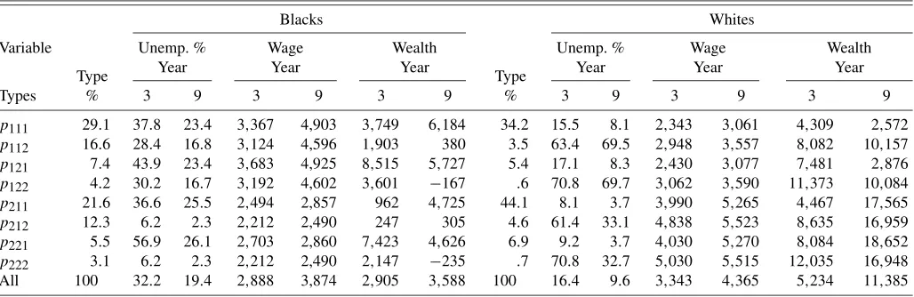
These probabilities for each subset of parameters produce eight combinations within each race group. However, four of these combinations alone cover 80% of blacks, whereas only two combinations represent altogether 78% of whites. For a better understanding of these combinations I also report unem-ployment rates, average quarterly wages, and wealth by race group and type combination for years 3 and 9 in Table 5.
For blacks type combination p111 equals 29% and is the
largest of this race group. It combines initially high job turnover, a relatively high wage offer distribution, and high wage growth with low wealth, tight borrowing constraints, high
transfers while unemployed, high risk aversion, and low disu-tility of working. This subset of the black population has high wages, which increase substantially over time, combined with the highest wealth levels and faster wealth accumulation of blacks. It also has relatively high unemployment levels, caused by the high reservation wages.
Type combinationp211of blacks represents 22% of its group,
the second largest. It exhibits the same features as the previous combination, except for the labor market environment, which produces lower mean accepted wages. Accordingly, unemploy-ment rates are higher, and wages and wealth levels over time are lower. Typep112, representing 16% of blacks, exhibits
fea-tures similar to type combinationp111, except for taste
para-meters: lower transfers while unemployed, lower risk aversion, and more disutility of working. Hence, this subset is more likely to work at lower wages and accumulate less, and thus exhibits lower unemployment rates, lower wages, and lower wealth lev-els. Finally, Typep212is the poorest segment of the blacks
sub-sample and covers 12% of blacks. It is characterized by low transfers while unemployed, low wages, and a labor market en-vironment in which it is hard to receive a job offer when un-employed, and easy to receive a job offer and get fired while employed. Accordingly, and despite the relatively high disutil-ity of working, reservation wages are relatively low, and there-fore, unemployment rates, wages, and wealth levels are rela-tively low. However, in spite of having the lowest wage levels among blacks, they exhibit a clear trend to accumulate wealth over the life cycle. This may be explained by the relatively low parameter for risk aversion and the tight borrowing constraint combined by the modest increases in wages over time.
In turn, there are two main type combinations among whites, p211with 44% andp111with 34% of individuals, which share
the same wealth and taste parameters. However, combination p211 enjoys in the long run a relatively more favorable labor
market environment with relatively low unemployment rates, and higher wages and wealth levels than combinationp111. This
last segment of the white sample faces a labor environment that is characterized by a reservation wage that is increasing in the agent’s wealth position, but with relatively low wage offers. This type combination faces a depressed labor market, char-acterized by an unemployment rate that is lower than the aver-age, but also with lower wages. This type combination is also
Table 5. Decomposition by types of selected predicted variables—unemployment rate, wages, and wealth by race, year, and type combination
Blacks Whites
Variable Unemp. % Wage Wealth Unemp. % Wage Wealth Type
characterized by low initial wealth, the lowest of whites, low disutility of working, and low risk aversion. However, because of the poor labor market, it exhibits low savings and decreasing wealth trajectories.
Comparing specific type combinations across race groups re-veals that they depict similar patterns in unemployment rates, wages, and wealth, just at different levels. For instance, the main single combination of each race group, p111 of blacks
andp211 of whites, shows a similar pattern of low unemploy-ment with important wage gains and wealth accumulation over time, more than the average in their respective race groups. The next important segment inside each race group shares wealth and taste parameters with these two main type combinations but has different labor market parameters associated with lower wages and lower wealth levels. Consequently, the most impor-tant source of heterogeneity for both race groups lies in the la-bor market rather than in wealth or taste parameters.
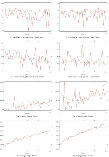
6. MODEL FIT
To assess how well these parameter estimates mimic the data, I compare the observed and the predicted choice distributions of employment status, employment transitions, wealth, and wages. Figures 3 and 4 show the actual and the predicted hazard rates for the first unemployment spell. For both groups, the model is able to replicate the data closely, especially for whites for whom the predicted hazard rate mimics closely the actual hazard rate and its negative duration dependence. However, for blacks the predicted hazard rate does not exhibit the pronounced negative duration dependence of its observed counterpart. This may be related to the increase in the observed hazard rate of blacks from quarter 11 until 13. A similar increase, though less abrupt, is also present in the hazard rate of whites from quarter 8 until 13. Since the initial wealth distribution and heterogeneity play a crucial role for reproducing this pattern, the few early wealth observations used in the estimation may be the reason the model does not reproduce closely the negative duration dependence of blacks. Conditional on initial wealth level and type, hazard rates are increasing over time: individuals reduce their wealth position while unemployed, so that reservation wages decline
Figure 3. Blacks’ hazard rates: first unemployment spell ( actual; predicted).
Figure 4. Whites’ hazard rates: first unemployment spell ( actual; predicted).
and hazard rates increase. However, because poorer individuals exhibit high hazard rates and are first to exit unemployment, the predicted average hazard rate tends to go down over time. Considering also that the observed hazard rates were not used in the estimation, this comparison can be considered a cross validation, an out-of-sample assessment of the model’s success in fitting the data.
Figure 5 offers a graphical comparison of all actual and predicted variables by quarter since graduation for both race groups. Additionally, Table 6 presents a summary of χt2 -statistics of the distributions of employment status and tran-sitions, wages, and wealth for years 3, 6, and 9 after gradu-ation for both race groups. Goodness-of-fit tests allow us to evaluate whether the theoretical model at the estimated pa-rameters can mimic the cell-by-cell distribution of the data. The test statistic across choices j at time t is defined as χt2=Jj=1(nj t − ˆnj t)2/nˆj t, wherenj t is the actual number
of observations of choicej at timet,nˆj tis the model predicted
counterpart,J is the total number of possible choices, andT is the number of years. This statistic has an asymptoticχ2 distri-bution withJ−1 degrees of freedom. This table also contains the predicted average wages and wealth levels and their associ-ated black–white ratios.
In the graphical comparison, the evolution of predicted em-ployment status and emem-ployment transitions replicates the ac-tual paths for both race groups very accurately: unemployment rates in Figures 5(a) and 5(b), transitions from unemployment to employment shown in Figures 5(c) and 5(d), job separations reported in Figures 5(e) and 5(f), and job-to-job transitions, in Figures 5(g) and 5(h). Observed exits from unemployment and job-to-job transitions are particularly noisy. The χ2 statistics corroborate this graphical evidence and show that prediction is accurate for both race groups: all of these variables pass theχ2 tests.
As illustrated by Figures 5(i) and 5(l) the model overpredicts slightly the percentage of layoffs in job separations, but predicts very accurately the percentage of layoffs in job-to-job transi-tions. Yet, at the formal level, the choice distributions of these transitions pass theχ2tests.
Figure 5. Actual and predicted paths by race group: employment status and employment transitions ( actual; predicted).
The corresponding evolution of wealth is illustrated graphi-cally in Figures 5(m) and 5(n). In spite of the noise in the wealth data, the model mimics well the observed pattern of wealth ac-cumulation. As implied by the initially decreasing hazard rate seen above, just after graduation whites decumulate wealth in order to finance their first unemployment spell, but then they ac-cumulate wealth as a result of making progress in their employ-ment careers. Blacks also show initial wealth decumulation, but it is not as pronounced as for whites. The model passes theχ2 tests for both race groups at all years. Recall from Table 1 that
the actual wealth of whites is more noisy than that of blacks. Nevertheless, the model reproduces relatively well the racial wealth ratio at the average, particularly at years 6 and 9, and its decreasing trend from year 6 to year 9.
As explained above, for most individuals in the sample initial wealth is not observed, as it is only observed from 1985 onward. This implies that conditioning on initial wealth in simulating the data for the goodness-of-fit tests is not feasible. Had such data been available, I could certainly have shown a better model fit.
Figure 5. (Continued). Actual and predicted paths by race group: layoffs, wealth, and wages ( actual; predicted).
Figures 5(o) and 5(p) show that wages are especially well replicated on average, with some overprediction for blacks and some underprediction for whites in later periods. The model also mimics well the observed wage distribution: it passes theχ2 tests for both race groups in all years, with the excep-tion of whites in year 9. The racial wage ratio is relatively well replicated, although its declining trend is only partially captured by the model, at year 3 and year 6.
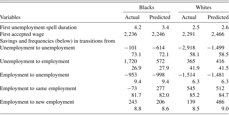
Table 7 shows the actual and predicted first unemployment spell duration and first accepted wage. It is shown that the
model is able to replicate these two variables pretty well, though with some underprediction of the unemployment duration of blacks and some overprediction of the first accepted wage of whites. This table also provides a comparison between observed and predicted savings by employment transitions as reported previously in Table 3. Comparing these predicted moments with their observed counterparts, as the hazard rates, is informative about the ability of the model to replicate observables that have not been used in the estimation. This table reveals a relatively good prediction of savings during job separations for both race
Table 6. Summary, blacks and whites: actual and predicted choice distribution—employment status and transitions, wealth, and wages for three selected years after graduation (in %)
Years after graduation
χ2 Blacks Whites
Year 3 6 9 3 6 9
Unemployment rate 1.1 12.6 .0 2.4 3.9 .6 Transitions from unemployment 1.1 1.7 2.1 .6 2.2 .3 Transitions from employment .1 5.1 4.6 1.3 .1 5.3 Quit-layoff rate in job loss 2.7 8.4 4.4 .2 4.5 1.8 Quit-layoff rate in job-to-job flow 3.2 .4 1.8 1.8 .0 4.3 Wealth distribution: 4.7 3.3 1.4 3.8 7.0 14.2 Predicted average wealth 2,905 3,064 3,588 5,234 6,014 11,385 Predicted black–white ratio 56 51 32
Wage distribution: 7.4 3.5 .5 2.1 8.5 22.4 Predicted average wage 2,888 3,415 3,874 3,343 3,948 4,365 Predicted black–white ratio 86 86 89
NOTE: Critical values at .5% significance:χ(21)=7.9,χ(22)=10.6,χ(23)=12.8,χ(24)=14.9.
groups, exits from unemployment and employment retention for whites, and job-to-job transitions for blacks. Other wealth variations by employment transitions are under- or overesti-mated. By contrast, the employment transitions themselves are very accurately predicted by the model.
In short, both graphically and formally, the model is fairly successful in replicating the main features of the data.
7. REGIME CHANGES AND DECOMPOSITION OF RACE GAPS
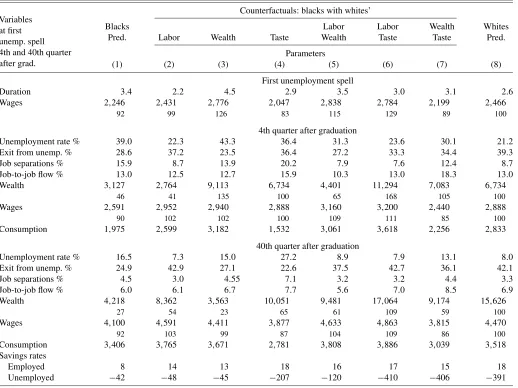
After recovering the underlying behavioral parameters, I ex-plore black–white variations of short- and long-term outcomes resulting from differences in the economic environment and in preferences as captured by the three subsets of parameters: first, assigning blacks the labor market conditions of whites, second, the initial wealth distribution and access to credit of whites, and, third, the taste parameters of whites. I also evaluate the
outcomes of performing two of these changes at a time. Educa-tion is assumed to be invariant to the regime changes considered here. In Appendix A8 I explain in greater detail how these ex-periments are performed.
The effects of these experiments are reported in Table 8, where the first and last columns show selected predicted vari-ables for the black and white subsample, respectively. Once again, average wages only contain the income of the employed. The first experiment, reported in column 2, addresses the im-portance of labor market conditions, that is, of the first subset of parameters in blacks’ outcomes. In this experiment, blacks face the same labor market conditions as whites. In the short term, the fourth quarter after high school graduation, this ex-periment narrows down the racial wealth gap very slightly: the black–white wealth ratio goes down from 46% to 41%. On the other hand, this experiment practically eliminates the ini-tial racial wage gap: in the fourth quarter the black–white wage ratio increases from 90% to 102%. Wealth does not initially converge substantially, because agents rely more on good
la-Table 7. Actual and predicted first unemployment duration, first accepted wage, and savings and frequencies in employment transitions
Blacks Whites Variables Actual Predicted Actual Predicted First unemployment spell duration 4.2 3.4 2.5 2.6 First accepted wage 2,236 2,246 2,291 2,466 Savings and frequencies (below) in transitions from
Unemployment to unemployment −101 −614 −2,918 −1,499 73.1 72.1 58.1 58.5 Unemployment to employment 1,720 572 365 416
26.9 27.9 41.9 41.5 Employment to unemployment −953 −998 −1,514 −1,481
9.4 9.4 6.3 6.3 Employment to same employment −73 277 545 512
81.7 82.0 85.2 84.7 Employment to new employment 243 206 139 486
8.8 8.6 8.5 9.0
Table 8. Regime changes: blacks with whites’ parameters Counterfactuals: blacks with whites’
Blacks Labor Labor Wealth Whites Pred. Labor Wealth Taste Wealth Taste Taste Pred.
Parameters Variables
at first unemp. spell 4th and 40th quarter
after grad. (1) (2) (3) (4) (5) (6) (7) (8) First unemployment spell
Duration 3.4 2.2 4.5 2.9 3.5 3.0 3.1 2.6 Wages 2,246 2,431 2,776 2,047 2,838 2,784 2,199 2,466
92 99 126 83 115 129 89 100
4th quarter after graduation
Unemployment rate % 39.0 22.3 43.3 36.4 31.3 23.6 30.1 21.2 Exit from unemp. % 28.6 37.2 23.5 36.4 27.2 33.3 34.4 39.3 Job separations % 15.9 8.7 13.9 20.2 7.9 7.6 12.4 8.7 Job-to-job flow % 13.0 12.5 12.7 15.9 10.3 13.0 18.3 13.0 Wealth 3,127 2,764 9,113 6,734 4,401 11,294 7,083 6,734
46 41 135 100 65 168 105 100
Wages 2,591 2,952 2,940 2,888 3,160 3,200 2,440 2,888
90 102 102 100 109 111 85 100
Consumption 1,975 2,599 3,182 1,532 3,061 3,618 2,256 2,833 40th quarter after graduation
Unemployment rate % 16.5 7.3 15.0 27.2 8.9 7.9 13.1 8.0 Exit from unemp. % 24.9 42.9 27.1 22.6 37.5 42.7 36.1 42.1 Job separations % 4.5 3.0 4.55 7.1 3.2 3.2 4.4 3.3 Job-to-job flow % 6.0 6.1 6.7 7.7 5.6 7.0 8.5 6.9 Wealth 4,218 8,362 3,563 10,051 9,481 17,064 9,174 15,626
27 54 23 65 61 109 59 100
Wages 4,100 4,591 4,411 3,877 4,633 4,863 3,815 4,470
92 103 99 87 104 109 86 100
Consumption 3,406 3,765 3,671 2,781 3,808 3,886 3,039 3,518 Savings rates
Employed 8 14 13 18 16 17 15 18
Unemployed −42 −48 −45 −207 −120 −410 −406 −391
bor market conditions and can afford to initially decumulate their initial wealth to finance their job search. These conditions also imply employment transitions and, therefore, unemploy-ment rates that are very similar to those of whites. In the long run, 40 quarters after graduation, the better labor market con-ditions prevail and wealth increases following wage increases, so that the racial wage ratio increases from 92% to 103%, and the racial wealth ratio from 27% to 54%. Although this last gap has importantly narrowed down, it remains relatively wide due to remaining differences in preferences.
As shown in column 3, having whites’ initial wealth distri-bution and access to credit increases blacks’ average wealth and wages in the fourth quarter after graduation, smoothing out racial differences almost completely: the racial wealth and wage ratio increase to 135% and 102%, respectively. It in-creases blacks’ consumption substantially in the fourth quarter after graduation. On the other hand, more initial wealth leads to a longer initial unemployment spell and higher rates of un-employment at the start of un-employment careers, deteriorating blacks’ employment situation. In the long run, racial dispari-ties do not diminish in wealth: 40 quarters after graduation the racial wealth ratio falls from 27% to 23%. Broader access to credit, unlike the displacement of initial wealth, is a
perma-nent change and undermines the need for holding wealth. How-ever, increased wages persist and become 99% of whites’. Thus, this experiment shows that increases in initial wealth do have a long-lasting effect in labor market outcomes.
The outcomes for blacks when they are assigned the taste pa-rameters of whites are presented in column 4. With more risk aversion, less disutility of working, and fewer transfers while unemployed, blacks become less selective in their job search and suffer an initial decline in the unemployment rate, from 39% to 36%, but an increase in accepted wages, from 90% to 100% of whites’ wages, and in wealth 46% to 100% of whites’. Despite this initial elimination of racial disparities in wealth and wages, consumption diminishes from $1,975 to $1,532, the lowest attained by any experiment. Forty quarters after gradu-ation, little is left from this full initial convergence in black– white ratios in wealth and in wages: the black–white wealth ra-tio becomes 65% and the black–white wage rara-tio becomes 87%. The unemployment rate rises to 27%, whereas in the baseline case it is only 17%.
The second set of experiments starts in column 5, combin-ing two changes at a time. This column illustrates the results of extending the first experiment by also assigning blacks the initial wealth distribution and borrowing possibilities of whites.
This variation increases blacks’ consumption, plus has the ini-tial effect of diminishing both the wealth and the wage gap: in the fourth quarter after graduation, relative wealth of blacks increases from 46% to 65% of whites’ and relative wages go up from 89% to 109%. However, the improved labor market conditions combined with looser borrowing constraints, both permanent changes, undermine the need of precautionary sav-ings, so that 40 quarters after graduation wealth does not ac-cumulate that fast and the racial wealth ratio increases from 27% to only 61%. At the same time, the wage gap disappears fully. Hence, this experiment is successful in achieving conver-gence in wages, but not in wealth, with an important increase in consumption: 40 quarters after graduation blacks’ average consumption has increased from $3,406 to $3,808, overtaking whites’ consumption of $3,518.
Had blacks the labor and taste parameters of whites, as re-ported in column 6, they would experience an important in-crease in their initial wealth: the racial wealth ratio rises from 46% to 168%. In this scenario, blacks’ first unemployment spell is shorter, their exit rates from unemployment higher, their un-employment rate lower, and their wages higher, even higher by 11% than whites. In the 40th quarter after graduation, this ex-periment has created full long-run racial convergence in wealth and wages: all wage and wealth gaps have disappeared. Given that borrowing constraints are the only remaining permanent difference with whites and that these are relatively tight and quite similar across race groups, this combined change is the most successful in eliminating wealth and wage racial differ-ences in the long run, so that the consumption level of blacks overtakes the consumption level of whites. Additionally, this experiment generates both faster wealth accumulation while employed and faster wealth decumulation while unemployed.
The combination of better initial wealth distributions, looser borrowing constraints, and the taste parameters of whites, re-ported in column 7, almost eliminates initial wealth racial dif-ferences. This convergence, however, does not prevail 40 quar-ters after graduation, as the wealth black–white ratio becomes 59%. However, this experiment has the effect of reducing the relative wage of blacks, initially from 90% to 85% and in the long run from 92% to 86% of whites’ wages. Unlike the sec-ond experiment, in which only initial wealth distributions and access to credit are increased, the current experiment also re-duces the disutility of working and transfers while unemployed, which results in lower reservation wages and, therefore, lower accepted wages. The increase in risk aversion, which has the effect of increasing reservation wages, does not seem enough to counteract this trend. Consequently, blacks do not have only lower wages, but also, and similarly to whites, lower unemploy-ment rates and employunemploy-ment transitions.
Another variable of interest in these experiments is the saving rate. Compared to blacks, whites save more when employed and dissave more when unemployed. Blacks’ savings rates in the long run converge to those of whites only when blacks are assigned the taste parameters of whites.
Summarizing, improving labor market conditions of blacks accomplishes initial and long-run convergence of labor market outcomes, that is, of wages, unemployment rates, and employ-ment transitions. If this improveemploy-ment is combined with a switch
in preferences, it also eliminates initial and long-run wealth dis-parity. On the other hand, improving the initial wealth distrib-ution and access to credit of blacks and changing their taste parameters are both regime changes that eliminate both racial wealth and wage gaps at the beginning of employment careers. However, none of these changes alone does diminish substan-tially the long-run racial wealth gap. Interestingly, increasing initial wealth does have a permanent effect in wages, it does reduce the racial wage gap, and accounts partially for the ob-served racial wealth disparity.
One can further use this set of experiments to decompose the total racial differences into the three parts considered here: labor market conditions, wealth, and preferences. The result-ing partitions are reported in Table 9. Appendix A9 details how these decompositions are performed.
Table 9 shows that labor market conditions are the most im-portant component underlying the racial differences in almost all variables. Initial wealth is important in accounting for racial wage differentials in the first unemployment spell. However, it has a persistent effect in accounting for job separations, job-to-job flows, wealth, and consumption. Preferences play a cru-cial role in explaining differences in exit from unemployment, job-to-job flows, wealth levels, and saving rates both while employed and while unemployed. Actually, the wealth gap is mostly determined by differences in preferences, followed in the short term by initial wealth, and by labor market conditions in the long term. These decompositions reinforce the message obtained previously that labor market conditions are the leading force underlying the observed racial differences. Differences in initial wealth and preferences are, however, crucial in explain-ing differences in some important variables that the labor mar-ket does not account for.
Table 9. Decomposition of observed racial gaps by differences in labor market, wealth, and tastes
8. CONCLUSIONS
The main purpose of this article has been to determine the extent to which initial wealth disparity is responsible for the observed differences in early employment careers of black and white individuals. I generalize Danforth’s (1979) utility-maximizing search model to allow for on-the-job search, wage growth, arrival and layoff rate variations, retirement, and a para-metric borrowing limit, and estimate it by a simulated method of moments using data from the NLSY. At the recovered behav-ioral parameters, the model mimics well the main observables, namely, the hazard rate during the first unemployment spell, first accepted wages, savings by employment transitions, and the cross-sectional distributions of wealth, wages, and employ-ment transitions over time.
Counterfactual experiments and decompositions of the racial differentials into labor market, wealth, and taste components reveal that most of the differences in labor market performance between blacks and whites several years after high school grad-uation are accounted for by differences in their wage offer dis-tributions and arrival and layoff rates, both in levels and growth, as well as preferences, in particular, the disutility of working. Differences in initial wealth do account for the racial gap in both wealth and wages at the beginning of employment careers; several years after high school graduation they account only for the racial wage gap, not the racial wealth gap. Thus, initial wealth does partially explain differences in early employment careers.
These results are revealing about racial differences in la-bor market outcomes stemming from initial wealth, the lala-bor market environment, and preferences. Throughout this article, I have abstracted from racial differences arising from schooling choices, which also provide insurance for labor risk (Whalley 2005), and general equilibrium effects, that is, regime changes can also affect wage offer distributions and arrival rates. The utility-maximizing job search model proposed here can be ex-tended in these two directions, which may alter the effects of regime changes implemented in this article. Recent articles by Lee (2005) and Lee and Wolpin (2006) account for school-ing decisions in a general equilibrium settschool-ing and are thus en-couraging about the feasibility of these extensions in future re-search.
ACKNOWLEDGMENTS
I thank Chris Flinn, Ken Wolpin, and Wilbert van der Klaauw for their suggestions to a previous version of this article. I am also grateful to Núria Quella, Hugo Ñopo, and participants of seminars at IZA, University of North Carolina–Chapell Hill, and at the LACEA conference of 2004 in Costa Rica, as well as to four anonymous referees. Financial support from the Spanish Ministry of Science and Technology grant SEC 2001-0674 and the Mexican Association of Culture is gratefully acknowledged. The usual disclaimer applies.
APPENDIX: PROOF OF PROPOSITION 1
I proceed inductively, showingwt+1(ω)≥bimplieswt(ω)≥ b, for t < T. Suppose that wt+1(ω)≥b andwt(ω)=b, for
t < T; then the value functions become Vte(At, b)
[Received May 2003. Revised December 2006.]
REFERENCES
Altonji, J. G., and Doraszelski, U. (2005), “The Role of Permanent Income and Demographics in Black/White Differences in Wealth,”Journal of Human Resources, 240, 1–30.
Blau, F., and Graham, J. W. (1990), “Black–White Differences in Wealth and Asset Composition,”Quarterly Journal of Economics, 105, 321–339. Bowlus, A., and Eckstein, Z. (2002), “Discrimination and Skill Differences
in an Equilibrium Search Model,” International Economic Review, 43, 1309–1345.
Danforth, J. P. (1979), “On the Role of Consumption and Decreasing Absolute Risk Aversion in the Theory of Job Search,” inStudies in the Economics of Search, eds. S. A. Lippman and J. McCall, New York: North-Holland, pp. 109–131.
Eckstein, Z., and Wolpin, K. (1989), “The Specification and Estimation of Dy-namic Stochastic Discrete Choice Models,”Journal of Human Resources, 24, 562–598.
Eckstein, Z., and Wolpin, K. (1999), “Estimating the Effect of Racial Discrimi-nation on First Job Wage Offers,”Review of Economic Studies, 81, 384–392. Fairlie, R. W. (1999), “The Absence of the African-American Owned Business: An Analysis of the Dynamics of Self-Employment,”Journal of Labor Eco-nomics, 17, 80–108.
Fairlie, R. W., and Meyer, B. D. (2000), “Ethnic and Racial Self-Employment Differences and Possible Explanations,”Journal of Human Resources, 35, 543–669.