Full Terms & Conditions of access and use can be found at
http://www.tandfonline.com/action/journalInformation?journalCode=ubes20
Download by: [Universitas Maritim Raja Ali Haji] Date: 12 January 2016, At: 00:15
Journal of Business & Economic Statistics
ISSN: 0735-0015 (Print) 1537-2707 (Online) Journal homepage: http://www.tandfonline.com/loi/ubes20
A Prior for Impulse Responses in Bayesian
Structural VAR Models
Andrzej Kocięcki
To cite this article: Andrzej Kocięcki (2010) A Prior for Impulse Responses in Bayesian
Structural VAR Models, Journal of Business & Economic Statistics, 28:1, 115-127, DOI: 10.1198/ jbes.2009.07278
To link to this article: http://dx.doi.org/10.1198/jbes.2009.07278
Published online: 01 Jan 2012.
Submit your article to this journal
Article views: 83
A Prior for Impulse Responses in Bayesian
Structural VAR Models
Andrzej K
OCI ˛ECKIEconomic Institute, National Bank of Poland, 11/21 Swietokrzyska, 00-919, Warsaw, Poland (andrzej.kociecki@mail.nbp.pl)
This article develops a comprehensive approach to formally introduce the prior for impulse responses into the Bayesian structural VAR (SVAR) models, with considerable attention paid to careful prior specifi-cation. Furthermore, we present an efficient algorithm to estimate the SVAR with a Gaussian prior for impulse responses using simulation methods. We also illustrate our methodology using an example in which we verifiy some facts concerning the impact of monetary policy shock on the economy.
KEY WORDS: Jacobian; Metropolis–Hastings algorithm; Monetary policy; Posterior.
1. INTRODUCTION
SVAR models are often used to recover the effects of mone-tary policy. If we are confronted with modeling of this kind, we often have strong prior beliefs about how the economy works. In particular, many economists seem to have a prior about some impulse responses. For example, there is a widely shared view that contractionary monetary policy shock (e.g., exogenous rise in the interest rate) should lower prices. If in the process of estimation we reach the opposite conclusion (so-called price puzzle), we reestimate the model changing the identifying re-strictions until the ultimate result is satisfactory. Paradoxically, even most of the Bayesian studies apply this informal use of prior knowledge. However, there is a danger that this may lead to circular reasoning—see Uhlig (2005), Faust (1998), and Gor-don and Boccanfuso (2001). We are left with precisely what we expected before the data analysis. Although this informal prior use has much appeal for some researchers (see, e.g., Leeper, Sims, and Zha1996), the others, like Uhlig (2005) and Faust (1998), called for the more formal treatment.
In particular, Uhlig (2005) and Faust (1998) applied sign restrictions on impulse responses. This amounts to simply re-stricting the support of impulse responses, but in some instances this approach may lack flexibility—within this framework we cannot specify the prior shape for impulse functions, for exam-ple, giving the central tendency and dispersion. In contrast, our approach accommodates such a case. Moreover the essential nature of sign restriction may be to some extent controversial: we do not allow the data to revise our prior, in the sense that when the data are in conflict with the prior we ignore the data.
The approach adopted herein has more in common with those of Dwyer (1998) and especially Gordon and Boccanfuso (2001). In contrast to Faust (1998) and Uhlig (2005), those authors worked with the prior for impulse responses by spec-ifying their shapes. In the article by Dwyer (1998) this is ac-complished with the help of a trinomial prior distribution. This certainly can be considered as a significant improvement in comparison with the sign restriction. However, Dwyer’s joint prior was a product of a relatively diffuse prior put on reduced form coefficients and trinomial distribution, whose properties are not lucid enough (both operate on distinct spaces, namely coefficients and impulse responses).
The work of Gordon and Boccanfuso (2001) is most closely related to our approach, at least taking into account the starting point. They argued that the most intuitive way to capture our prior about impulse function is to describe its central tendency and dispersion around it; sufficient for reaching this goal is a multivariate normal distribution.
The problem with their approach is that it is simply fun-damentally unsound. They tried to approximate a nonstandard prior on coefficients space (induced by the prior for impulse re-sponses) with a normal distribution, which as we shall see later, is incorrect.
As argued above, all the just-mentioned studies do not offer fully satisfactory approaches to deal formally with the prior for impulse response within a VAR framework. That may be sur-prising to some extent, especially when one adopts the Bayesian perspective. Indeed, as impulse responses are functions of coef-ficients there is, in principle, an obvious way to accomplish this: the researcher must translate only the prior regarding impulse responses shape, which is formalized by some prior probability density function (pdf), into the space of coefficients. Then, one obtains the implied prior pdf for coefficients and the Bayesian analysis can be used to update the prior knowledge. In practice, matters are more complicated. As emphasized by Sims (2002), the problem lies in the highly nonlinear mapping between im-pulse response functions and the structural coefficients. Indeed, in order to make the formal transformation between these two spaces we should obtain the Jacobian, which was thought to be analytically intractable. Our important contribution is to show that using appropriate representation of impulse responses it is surprisingly easy to write down this Jacobian. It turns out that the Jacobian has a simple form involving only the coefficients on contemporaneous relations among variables. This allows us to apply the Bayesian methods very easily, for the straightfor-ward simulation becomes feasible. In particular, we show how it can be done when one adopts a Gaussian prior for impulse responses.
© 2010American Statistical Association Journal of Business & Economic Statistics
January 2010, Vol. 28, No. 1 DOI:10.1198/jbes.2009.07278
115
2. THE MODEL AND NOTATION
We work with the popular model called structural VAR (SVAR):
A0yt=c+A1yt−1+A2yt−2+ · · · +Apyt−p+εt, (1) whereyt:m×1 are observables, A0:m×m is (nonsingular) matrix of coefficients measuring the contemporaneous relation betweenyt,c:m×1 is a vector of constants, andA1, . . . ,Ap arem×mmatrices of coefficients on lagged data. For structural shocks we assumeεt∼N(0,Im). Next, we find it useful to in-troduce some notation:Fm×l=[A1 A2 · · · Ap c] where l=mp+1,Y′=[y1 y2 · · · yT],T denotes sample size and
X′=
⎡
⎢ ⎢ ⎢ ⎢ ⎣
y0 y1 · · · yT−1
y−1 y0 · · · yT−2
..
. ... . .. ...
y−p+1 y−p+2 · · · yT−p
1 1 · · · 1
⎤
⎥ ⎥ ⎥ ⎥ ⎦
.
Given any nonsingular matrix Z, its determinant will be de-noted by det(Z)or|Z|, the latter being reserved only for posi-tive definite matrices. In the context of Jacobians, we will also need an absolute value of the determinant which will be denoted by |det(Z)|.J(Z→S)is Jacobian of transformation from Z toS. Furthermore D,p(·), andP(·|D)denote the data, a prior distribution, and a posterior distribution, respectively. Since in our development we will sometimes be concerned with the pos-terior under the flat prior, to avoid some confusion we will sys-tematically denote such a posterior with a subscript 0, that is, P0(·|D). Multivariate normal pdf with meanaand covarianceb will be denoted N(a,b).
3. THE POSTERIOR UNDER A FLAT PRIOR
When we take a flat prior for all structural coefficients, the posterior is proportional to the likelihood function
P0(A0,F|D)∝ |det(A0)|T
×etr
−12(A0Y′−FX′)(A0Y′−FX′)′ , (2) where etr{·} =etr{·}, and tr is a trace operator. Exploiting known decomposition of the term in braces we have
P0(A0,F|D)
∝ |det(A0)|T
×etr−12A0QA′0− 1
2(F− ˆF)X
′X(F− ˆF)′ , (3)
whereQ=Y′[IT−X(X′X)−1X′]Y;Fˆ=A0Y′X(X′X)−1. Accordingly, we factorized our posterior into the conditional posterior ofFgivenA0:
P0(F|A0,D)∝etr−12(F− ˆF)X′X(F− ˆF)′ (4) and the marginal posterior forA0:
P0(A0|D)
∝ |det(A0)|Tetr−12A0QA′0
= |det(A0)|Texp−12vec(A0)′(Q⊗Im)vec(A0) . (5) As far as the marginal posterior forA0, that is, (5), is concerned, we note that this is not a nonstandard pdf, as argued, for exam-ple, by Sims and Zha (1999). Indeed, Koci˛ecki (2005) showed
that (5) is the matricvariate generalization of the multivariate “symmetric Kotz type” distribution. See Koci˛ecki (2005) for further details.
On the other hand, in the case of the conditional posterior of FgivenA0, that is, (4), there is no any ambiguity: it is a matric-variate normal pdf. For our purposes, it is important to decom-pose (4) in a way that it will facilitate the efficient simulation from the posterior under the impulse responses prior. To this end, using the “vec” operator applied toFin the matricvariate normal pdf (4), we have
P0(F|A0,D)∝etr−12X′X(F− ˆF)′(F− ˆF)
=exp
−12(vec(F)−vec(Fˆ))′
×(X′X⊗Im)(vec(F)−vec(Fˆ)) =N(vec(Fˆ), (X′X)−1⊗Im). (6) SinceF=[A1 A2 · · · Ap c], we get
vec(F)=
⎡
⎢ ⎢ ⎢ ⎢ ⎣
vec(A1) vec(A2)
.. .
vec(Ap) c
⎤
⎥ ⎥ ⎥ ⎥ ⎦
.
Thus, the conditional posterior of vec(F)givenA0obeys a mul-tivariate normal law, that is, (6). Importantly,cand vec(Ai), for
i=1, . . . ,p, enter vec(F)in such a way that it permits us to
decompose (6) as
P0(F|A0,D)=P0(c|vec(Ap), . . . ,vec(A1),A0,D)
× p
k=1
P0(vec(Ak)|vec(Ak−1), . . . ,A0,D), (7) where all the above conditional densities are also multivariate normal. In particular,
P0(Ak|Ak−1, . . . ,A0,D)=N(μk,k) (8)
fork=1,2, . . . ,p, and
P0(c|Ap,Ap−1, . . . ,A0,D)=N(μc,c). (9) Since explicit formulas forμk,μc,k,c require tedious no-tation we omit them from our exposition. Needless to say, they may be found in any econometric or statistics textbook.
4. THE PRIOR FOR IMPULSE RESPONSES
Now we take up the issue of proposing the prior for impulse response functions. Let us denote byk,m×mmatrix of im-pulse responses afterk periods of time,0 being the instan-taneous response. In particular,ψij,kis theith row,jth column generic entry ofk (according to our conventionψij,k is sim-ply the response of theith variable to thejth shockεjt afterk periods). In our framework, we introduce the prior only for the first p+1 impulse responses, that is, 0,1, . . . ,p. How-ever, it is evident that those firstp+1 impulse responses matri-ces uniquely define all remaining impulse responses in periods
p+1,p+2, . . . .Taking this perspective, if we assign the prior
for0,1, . . . ,p, it is neither needed nor recommendable to
put explicitly a prior forp+1, . . .(since we may get some in-coherence).
Since each i is a matrix, we will work with its vector-ized form, that is, vec(i). As the most general prior setup, we consider the joint normal prior for impulse responses
0,1, . . . ,p, and for more transparency we write this prior
where all symbols with a bar above (and throughout this ar-ticle) indicate known parameters of the prior (i.e., hyperpara-meters). Thus, the above prior allows for specifying the prior central tendency for each generic entryψij,k (specific elements in¯k), the prior variance of eachψij,k (diagonal elements of
¯
Vkk), cross–correlations between responses to any shock in the kth period after the shock (off–diagonal elements ofV¯kk), and time–correlations between any response to a given shock, that is, impulse response smoothness (diagonal elements V¯ij for i=j).
Because (10) is a multivariate normal distribution, we can decompose it as follows:
To save the space, we omit explicit expressions forθk andkk as they may be found in any textbook that contains even ele-mentary facts about normal pdf. Suffice it to say thatkk is only a function ofV¯ij(for 0≤i≤k,0≤j≤k), whereasθkis a function of the hyperparameters andA0,A1, . . . ,Ak−1.
5. THE JACOBIANS FROM IMPULSE RESPONSES TO THE COEFFICIENTS
In the previous section we laid down the prior for impulse re-sponses. The complication arises because the likelihood is spec-ified in terms of the structural coefficients, whereas the prior (10) operates on the space of impulse responses. In order to formally use (10) along with the data via the Bayes formula, we should provide the link between the impulse response prior (10) and the induced prior defined on the structural coefficients space. The key is the Jacobian of transformation between these
two spaces. To this end, we adopt the following recursive repre-sentation for impulse responses, which will prove essential for an easy derivation of the Jacobian:
0=A−01, to–one relation between firstp+1 impulse responses, that is,
0,1, . . . ,p, andA0,A1, . . . ,Ap, from which we have the
following proposition.
Proposition 1. The Jacobian of transformation from impulse responses to structural coefficients is:
(a) forA0withm2functionally independent elements:
J(0,1, . . . ,p→A0,A1, . . . ,Ap)= |det(A0)|−2m(p+1) (b) forA0lower or upper triangular:
J(0,1, . . . ,p→A0,A1, . . . ,Ap)= |det(A0)|−(2mp+m+1) wherea0iiis theiith (diagonal) element ofA0
(c) forA0lower or upper triangular with 1’s on diagonal:
J(0,1, . . . ,p→A0,A1, . . . ,Ap)=1. Proof. See AppendixA.
There is a direct connection between the various cases cov-ered by Proposition 1 and the issue of SVAR identification. Leaving aside the long–run restrictions, the common practice is to achieve the identification by imposing the short–run re-strictions. That is, to restrict onlyA0. Indeed, we must provide with at least m(m2−1) independent restrictions to produce the meaningful and unambiguous SVAR analysis. Seen from this perspective, the case (a) is useless from the practical point of view. On the other hand, if one takes seriously the suggestions made by Drèze (1972,1974) we should not constrain ourselves to the dogmatic restrictions; probabilistic restrictions will serve the purpose. Indeed, this possibility was long ago thought as an attractive potential of Bayesian approach to econometrics, see, for example, the remarks by Drèze (1972, 1974, 1976). Thus, in principle, by appropriate incorporation of the prior pdf’s into the Bayesian analysis (that express the probabilis-tic restrictions), the problem of identification may be properly addressed.
The case (b) is relevant when one adopts the recursive iden-tification scheme. The case (c) covers essentially the same scheme, but in addition assumes that the diagonal elements inA0are set to 1. It will be of interest if imposing the recur-sive identifying scheme, instead of the variance normalization,
one chooses the coefficients normalization in (1). Of course, in this case the shocks variances are not normalized.
As a general remark why the proposition covers essen-tially only the recursive restrictions, note that there is an in-trinsic, fundamental problem with changing variables from
0,1, . . . ,ptoA0,A1, . . . ,Ap. It implicitly requires a Ja-cobian transformation fromA−01toA0—see AppendixA. Un-lessA0posits an appropriate identifying scheme, for example, the recursive one, the number of functionally independent ele-ments inA−01andA0do not need to be equal. If this is the case, the Jacobian vanishes. For instance, the number of excluding restrictions in A−01 do not need to be equal to the number of implied “zeros” inA0.
Proposition 1 covers essentially only the case of recursive identification. Although this is very popular in applied work— see, for example, Christiano, Eichenbaum, and Evans (1999) and our Section 8—this certainly does not exhaust all strate-gies used in many studies. As nonrecursive identifying schemes are now in widespread use, one may ask the question about the usefulness of Proposition 1 in practical applications. Un-fortunately, the methodology developed in this article allows only for recursive identification schemes (unless one has no ob-jections to using probabilistic restrictions). However, we con-jecture that our approach may be extended to accommodate any nonrecursive identifying schemes. To justify this claim, note that careful analysis of the proof of Proposition 1 sug-gests that the knowledge of the identifying scheme of A0 is needed only for a derivation of the Jacobian fromA−01toA0. In other words, if we adopt any nonrecursive identifying scheme we may simply state the prior not for impulse response func-tions 0,1, . . . ,p, but for A0,1, . . . ,p. Then, there is no need to change variables from A−01 to A0, and the re-quired Jacobian readsJ(A0,1, . . . ,p→A0,A1, . . . ,Ap)= J(1, . . . ,p→A1, . . . ,Ap), and the particular identification scheme put onA0plays no role in the derivation of the latter Jacobian.
The fact that Jacobians from Proposition1 involve onlyA0 has far-reaching consequences for the analysis. Actually, it greatly simplifies the simulation from the posterior. Of course, the key implicit assumption in all these Jacobians is that we change variables between first p impulse responses and the structural coefficients. That is, it allows for explicit expression of prior belief about the impulse responses’ shapes only forp periods after the shock. Evidently, when one tries to incorpo-rate directly the prior for long–run responses, the convenient setup breaks down. For example, consider the case when all variables in SVAR are nonstationary, that is,I(1), and there is no cointegration between those variables. Then the long–run response is given by ∞=(A0−A1−A2− · · · −Ap)−1. When one wants to state the prior directly for this long–run effect, one should be able to derive the Jacobian that explic-itly involves∞. To this end, assume that we adopt the
recur-sive identifying scheme [case (b) from Proposition1], then one way to conduct the analysis is to exploit the following Jacobian (which may be derived using partial results in AppendixA):
J(0,1, . . . ,p−1,∞→A0,A1, . . . ,Ap)
= |det(A0)|−2mp+m−1
det
A0− p
i=1
Ai
−2m
. (15)
Note that in contrast to Proposition1, the above Jacobian de-pends on all SVAR coefficients. Thus it destroys a convenient framework and appearance of such a Jacobian makes the poste-rior simulation more demanding (though of course possible).
6. AN IMPLIED PRIOR FOR STRUCTURAL COEFFICIENTS
Having obtained appropriate Jacobians, we are in a position to derive the induced prior for SVAR coefficients. Following (11), (12), and (13) we write
p(0,1, . . . ,p)∝exp
−1
2(vec(0)−vec(¯0))
′
× ¯V−001(vec(0)−vec(¯0))
× p
k=1 exp
−1
2(vec(k)−θk)
′
×−kk1(vec(k)−θk)
. (16)
Our task is to express the above prior in terms of the structural coefficients. To this end, we apply the vec operator to the recur-sive representation of impulse responses (14), which yields
vec(0)=vec(A−01),
vec(1)=(A′−0 1⊗A−01)vec(A1), vec(2)=vec(B11)+(A′−0 1⊗A−
1
0 )vec(A2),
vec(3)=vec(B12+B21)
(17) +(A′−0 1⊗A0−1)vec(A3),
.. .
vec(p)=vec(B1p−1+B2p−2+ · · · +Bp−11)
+(A′−0 1⊗A0−1)vec(Ap).
Fork=2, . . . ,p, we arrive at the general expression
vec(k)=vec(f(A0,A1, . . . ,Ak−1))
+(A′−0 1⊗A0−1)vec(Ak), (18) where f(·) is a function of only denoted arguments, that is, f(A0,A1, . . . ,Ak−1)=B1k−1+B2k−2+ · · · +Bk−11. Notice that vec(k)givenA0,A1, . . . ,Ak−1is linear in vec(Ak). As a result, the induced conditional prior for vec(Ak) given A0,A1, . . . ,Ak−1may be easily derived.
To complete the prior, we have to obtain the Jacobian from
0,1, . . . ,ptoA0,A1, . . . ,Ap. To this end, we should first decide on the identifying scheme forA0. As emphasized in the previous section, our framework essentially allows for only re-cursive identifying scheme. Of course, there remains an option with all restrictions introduced in a probabilistic manner; how-ever, we illustrate our approach only with the recursive identi-fying scheme.
Changing the variables in (16) from 0,1, . . . ,p to
A0,A1, . . . ,Apaccording to (17), and taking into account the
Jacobian (b) from Proposition1, we have
p(A0,A1, . . . ,Ap)
∝ |det(A0)|−(2mp+m+1)exp
−1 2(vec(A
−1
0 )−vec(¯0))
′
× ¯V−001(vec(A0−1)−vec(¯0))
× p
k=1 exp
−1
2(vec(Ak)−vec(¯¯k))
′
× ¯¯V−k1(vec(Ak)−vec(¯¯k))
∝ |det(A0)|−(m+1)exp
−1 2(vec(A
−1
0 )−vec(¯0))
′
× ¯V−001(vec(A0−1)−vec(¯0))
× p
k=1
| ¯¯Vk|−1/2exp
−1
2(vec(Ak)−vec(¯¯k))
′
× ¯¯V−k1(vec(Ak)−vec(¯¯k))
, (19)
where ¯¯
V−k1=(A−01⊗A′−0 1)−kk1(A′−0 1⊗A−01), (20) vec(¯¯1)=(A′0⊗A0)θ1, (21) vec(¯¯k)=(A′0⊗A0)
θk−vec(f(A0,A1, . . . ,Ak−1))
fork=2, . . . ,p, (22)
and vec(f(A0,A1, . . . ,Ak−1)) is defined as in (18). More-over, as noticed in Section 4, θk is also only a function of
A0,A1, . . . ,Ak−1 (and hyperparameters). Therefore, an
im-plied joint prior for structural coefficients may be decomposed
p(A0,A1, . . . ,Ap)
=p(A0)× p
k=1
p(vec(Ak)|vec(Ak−1), . . . ,A0) (23) that is to say, into the marginal (nonstandard) prior forA0:
p(A0)∝ |det(A0)|−(m+1)exp−12(vec(A0−1)−vec(¯0))′
× ¯V−001(vec(A0−1)−vec(¯0)) , (24) and successive conditionals forA1, . . . ,Ap, all of which obey multivariate normal law:
p(vec(Ak)|vec(Ak−1), . . . ,A0)=N(vec(¯¯k),V¯¯k)
fork=1, . . . ,p. (25)
Note that the prior expressed in terms of impulse responses does not induce any prior for deterministic terms, for exam-ple, constant. That is why the joint prior (23) does not involve the prior for a constant. To complete the prior specification we need a prior for constant terms (it should be understood that
the term “constant” may accommodate deterministic trends and dummies, which may be taken into account with no special ef-fort). We introduce the prior forcas follows:
p(c,A0,A1, . . . ,Ap)
=p(A0,A1, . . . ,Ap)×p(c|Ap,Ap−1, . . . ,A0). (26) There are two apparent, practical alternatives for expressing the prior in this framework. The first one is to assume a flat prior forc. The problem that arises in such a case is well recognized, and even if we are able to control the variance ofc(with the help of prior shrinking hyperparameters), the flat prior forcis not, however, a sensible choice in an applied work. Indeed, de-pending on the sum of reduced form coefficients, the constant changes its interpretation. For a stationary system, the constant relates to the mean of {yt}, but in a nonstationary or cointe-grated system the constant determines the drift in{yt}. In the latter case we may want to exclude the linear trends from data-generating process, thus forcec→0. The reason why the prior forcshows up as conditional on the coefficients originates from this concern—see Schotman and van Dijk (1991) for a discus-sion related to univariate AR process, and especially Sims and Zha (1998) for elaboration on VAR models. Following the idea of “dummy” observations of Sims and Zha (1998), we propose the prior
p(c|Ap,Ap−1, . . . ,A0)=N(c¯, λ−1Im), (27) wherec¯=A0(Im−pi=1Bi)y; ¯¯ y=1ppi=1y−i+1andλis non-negative (scalar) hyperparameter which governs the precision of the prior normal pdf. The larger λ, the more concentrated the prior aroundc¯. Ifλapproaches 0, the prior becomes more spread out (ifλ=0 we have a flat prior). For the rationale be-hind this prior and its detailed discussion we refer to Sims and Zha (1998). Suffice it to say that the prior (27) implies that E(yt)=0, irrespective of whether the data are stationary or nonstationary (with or without cointegration). Thus in any case, the prior assigns skepticism about linear trends, which in rela-tively large systems may be a key assumption for making good forecasts; see Sims (1996).
In addition, we can extend the above joint priorp(A0,A1,
. . . ,Ap)in a Minnesota–like shrinking prior, designed for the
structural VAR’s by Sims and Zha (1998). Notice that such a prior carries the smoothness assumption for impulse responses. Indeed, using recursive representation of impulse responses matrices it is easy to see, as the Minnesota prior becomes more and more concentrated (by setting appropriate variance hyper-parameters), that E(i|A0)≃0, where expectation is taken with respect to the prior (normal) pdf. If we do not explic-itly introduce the smoothness assumption (impulse responses time–correlations), that is, if we set V¯ij=0 for i=jin (10), a Minnesota prior of Sims and Zha (1998) would be a useful extension to our framework.
7. THE POSTERIOR ANALYSIS
The framework adopted in previous sections allows us the following decomposition of the joint posterior:
P(c,A0,A1, . . . ,Ap|D)
=P(A0|D)×P(A1|A0,D)× · · · ×P(Ap|Ap−1, . . . ,A0,D)
×P(c|Ap,Ap−1, . . . ,A0,D). (28)
Importantly, all the above densities are standard, except the marginal posterior ofA0. In particular
P(A0|D)∝ |det(A0)|T−(2mp+m+1)
×exp
−1
2vec(A0)
′(Q⊗I
m)vec(A0)
×exp
−1 2(vec(A
−1
0 )−vec(¯0))
′
× ¯V−001(vec(A0−1)−vec(¯0))
× p
k=1
|−k1+ ¯¯V−k1|−1/2 (29)
P(Ak|Ak−1, . . . ,A0,D)=N(μ˜k,˜k)
fork=1, . . . ,p, (30)
P(c|Ap,Ap−1, . . . ,A0,D)=N(μ˜c,˜c); (31) see AppendixBfor a derivation and formulas forμ˜k,μ˜c,˜k,
˜
c.
Now we comment on the marginal posterior for A0. Note that the covariance terms of prior beliefs about impulse shapes, that is, V¯ij, enter directly the marginal posterior of A0 (via
¯¯
V−k1)—see (20) and Section 4. This is a very attractive fea-ture as it provides a direct link between prior beliefs about impulse shapes in periods 1, . . . ,p and the marginal poste-rior for A0. Furthermore, even with a flat prior for 0, the marginal posterior is no longer invariant under an orthog-onal rotation of A0. This is due to the last product term in (29). It implies that being informative about the impulse responses we effectively identify the structure under consid-eration. Indeed, using the concept of D-identification of Flo-rens, Mouchart, and Richard (1974), one may show thatA0is D-identified.
Taking into account the posterior decomposition (28), the ef-ficient sampling from the joint posterior (under the Gaussian prior for impulse responses) is self–evident but for the reader’s convenience we state this algorithm explicitly:
1) DrawA0from nonstandard marginal posteriorP(A0| D); see (29).
2) Having A0, draw vec(A1) from m2–variate condi-tional normal distributionP(A1|A0,D)=N(μ˜1,˜1); see (30).
3) Having A0 andA1, draw vec(A2) from m2–variate conditional normal distribution P(A2|A1,A0,D)= N(μ˜2,˜2); see (30).
· · ·
p+1) Having A0,A1, . . . ,Ap−1, draw vec(Ap) from m2– variate conditional normal distribution P(Ap|Ap−1,
. . . ,A0,D)=N(μ˜p,˜p); see (30).
p+2) HavingA0,A1, . . . ,Ap, drawcfromm–variate con-ditional normal distribution P(c|Ap,Ap−1, . . . ,A0, D)=N(μ˜c,˜c); see (31).
p+3) Go to 1).
A closer look at the structure of the conditional posteri-orsP(Ak|Ak−1, . . . ,A0,D)from the above algorithm will re-veal that during each iteration the computation of these condi-tional densities involves only inverses of matrices of dimension m2×m2. Thus, the proposed sampling is quite efficient in com-parison with the (brute) joint sampling of A1, . . . ,Ap at one time, which would entail the inverses of much larger matrices (at each iteration).
As far as the marginal posterior for A0 is concerned, presently there are many alternatives to sample from any non-standard pdf; for example, Metropolis–Hastings (M–H) algo-rithm, hit–and–run sampler of Chen and Schmeiser (1996), or, recently proposed by Bauwens et al. (2004), adaptive polar sampling. In particular, in an example from Section8, to sample fromP(A0|D)we used an Independence M–H algorithm.
8. EMPIRICAL ILLUSTRATION
As an application of our framework we will verify some facts about the responses of key macroeconomic variables to the monetary policy shock. As an illustration we use the dataset employed in many studies, for example, Bernanke and Mihov (1998), Leeper, Sims, and Zha (1996), and importantly in Uh-lig (2005). We estimate 6 variable SVAR (with 12 lags) for the U.S. with real GDP(Y), the GDP deflator(P), a commodity price index (PC), total reserves (TR), nonborrowed reserves
(NBR), and the federal funds rate(RF). The data are monthly from 1965:01 to 1996:12.
Although we are aware of many identifying schemes rel-evant to our dataset—for example, Strongin (1995), Leeper, Sims, and Zha (1996), Bernanke and Mihov (1998), and Chris-tiano, Eichenbaum, and Evans (1999)—the recursive scheme was tested by many researchers dealing with this dataset and seems to work well as far as impulse responses are concerned. See, for example, Faust (1998), Christiano, Eichenbaum, and Evans (1999), and Leeper, Sims, and Zha (1996) (needless to say, our framework is well suited only for the recursive specifi-cation).
As is well known, the order of variables in the system in-fluences the resulting impulse responses. We estimated the SVAR with the orderingY,P,PC,NBR,RF,TR, which accord-ing to the above studies may be reasonable. The main under-lying assumption is that there is no immediate feedback from the policy variables (NBR,RF,TR) to the economy (Y,P,PC). For measuring the effects of monetary policy we shall at-tribute to a single equation shock, the label “monetary policy shock.” In particular, we identify the monetary policy shock with the fourth equation innovation (NBR), as motivated by Faust (1998), Christiano, Eichenbaum, and Evans (1999), and Leeper, Sims, and Zha (1996).
To proceed further, we shall incorporate the prior for impulse responses. Because we are interested in the effects of mone-tary policy, we shall be informative only with respect to the responses of all variables to the monetary policy shock. The ef-fects of all other shocks will be given a diffuse prior (large stan-dard deviation in normal pdf). Taking into account that all vari-ables (except the interest rate) are in logarithms, we propose the prior central tendency of responses to monetary policy shock as shown in Table1.
These reflect the common view that following a contrac-tionary monetary policy shock, all macroeconomic categories
Table 1. Prior mean responses to monetary policy shock
Horizon Y P PC NBR RF TR
1 −0.001 −0.001 −0.002 −0.005 0.3 −0.002
2 −0.0012 −0.0011 −0.003 −0.007 0.32 −0.0025
3 −0.0014 −0.0012 −0.004 −0.0072 0.33 −0.003
4 −0.0016 −0.0013 −0.005 −0.007 0.32 −0.0035
5 −0.0018 −0.0014 −0.006 −0.0065 0.30 −0.004
6 −0.0020 −0.0015 −0.0065 −0.006 0.25 −0.0042
7 −0.0021 −0.00155 −0.007 −0.0055 0.23 −0.0043
8 −0.0022 −0.0016 −0.0075 −0.005 0.21 −0.0044
9 −0.0023 −0.00165 −0.008 −0.0048 0.18 −0.0043
10 −0.00235 −0.0017 −0.0085 −0.0045 0.15 −0.0042
11 −0.00237 −0.00172 −0.009 −0.004 0.14 −0.0041
12 −0.00239 −0.00174 −0.0095 −0.0039 0.13 −0.004
listed in the table should decrease, except the interest rate, which should rise. Of course, we are not dogmatic, as we at-tribute to each mean response a prior uncertainty (variance) and in particular we shall be interested in how this uncertainty contributes to the posterior shape of impulse responses. Since an elicitation of the covariance matrix is the hardest task we assumed that all impulse responses are independent, that is,
¯
Vij=0for i=jand eachV¯ii is diagonal—see (10). Thus, we only specify the prior means and variances. Of course this is far from a realistic assumption. We decided to do so because we treat our empirical analysis only as an illustration of the econo-metric framework. In real applications, if one has some knowl-edge about the cross–correlations and/or time–correlations be-tween variables responses to any given shock, one can easily in-corporate it into the prior since our framework allows for such a general prior covariance. In general, the knowledge about some impulse responses may come from an economic model, for ex-ample, DSGE.
In the first exercise, a relatively diffuse prior on responses has been imposed. A normal prior with a standard deviation 0.01 for all impulse functions listed in Table1, except the fed-eral funds rate where standard deviation was set to 0.4. This prior, although concentrated around the means listed in Table1, has rather ambiguous implications: the responses’ shapes are not essentially determined (for every impulse function and each period, 0 line is well within±one prior standard deviation from the prior mean). Furthermore, we assumed a flat prior for con-temporaneous responses0=A−01(which itself is lower trian-gular).
As emphasized in Section7, the main inferential problem re-lates to the nonstandard form of the marginal posterior forA0. Since we decided to be noninformative with respect to the unre-stricted entries in lower triangularA−01, it follows that our target function will be the marginal posterior forA0, that is, (29), but without the term being the kernel of a prior distribution forA−01, that is,
P(A0|D)∝ |det(A0)|T−(2mp+m+1)
×exp
−1
2vec(A0)
′(Q⊗I
m)vec(A0)
× p
k=1
|−k1+ ¯¯V−k1|−1/2.
(32)
To draw from P(A0|D)we used an Independence M–H algo-rithm and for its detailed description the reader is referred to AppendixC.
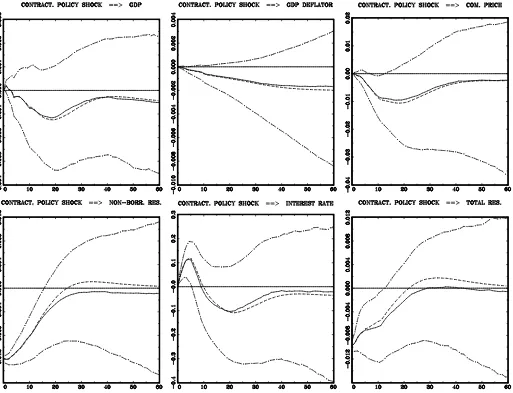
The posterior results are shown in Figure1. Impulse function analysis was based on (effectively) 5,000 draws from the pos-terior. Although it is a relatively small number of simulations it turned out to be sufficient. We also note that a version of the Minnesota prior designed for SVAR by Sims and Zha (1998) was used in all computations in this article. Each horizontal axis is the response period in months. A solid line is a median re-sponse, and two (long) dashed lines are error bands that contain 68% (pointwise) posterior probability mass. In addition, a short dashed line is the response evaluated at the posterior mean of structural coefficients. The central tendency in all cases is con-sistent with the common view. This should not be a surprise, since the identifying scheme adopted here has been subject to careful investigation in many previous studies and turned out to be credible. However, for economic reasoning, it is important to have a paralleled confirmation in terms of probability that these impulses are at least of a given sign. With such a diffuse prior we are quite confident that the federal funds rate immediately goes up, nonborrowed and total reserves are decreasing after the contractionary monetary policy shock and perhaps commodity prices are decreasing with some delay, reaching a minimum, say, 18 months after the shock.
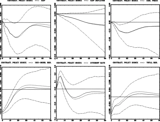
The situation changes qualitatively if we tighten the prior for impulse responses. Specifically, using the same prior means as in Table1, we set the prior standard deviations to 0.0015 for GDP and the GDP deflator, 0.005 for a commodity price in-dex, total reserves, nonborrowed reserves, and 0.1 in case of the federal funds rate. The results are shown in Figure2. Now all impulse functions are, with 68% probability (for some period after the shock), properly behaved. The GDP deflator decreases permanently, GDP remains negatively influenced for some pe-riod (roughly after one year and a half), total reserves are evi-dently negatively responding, and the commodity prices index is even more sharply determined. We notice that we do not ob-serve “price puzzles,” that is, prices move up after a contrac-tionary policy shock, which were quite frequently encountered in the studies that used the same dataset. However, we do ob-serve a tiny “output puzzle,” that is, GDP goes up after a con-tractionary policy shock. However, in comparison with other empirical studies, the amount of this “puzzle” is hardly seen.
Figure 1. Responses of all variables to a contractionary, one standard deviation, monetary policy shock. A lower triangular form forA0was
assumed. A relatively diffuse prior on responses has been applied (standard deviation of 0.01 for all impulse functions, except the federal funds rate where standard deviation was set at 0.4). The prior means as in Table1. Each horizontal axis is the response period in months. The solid line is the median response, and two (long) dashed lines are error bands that contain 68% (pointwise) posterior probability mass. In addition, the short dashed line is the response evaluated at the posterior mean of structural coefficients.
As far as the overall shape of the GDP response is concerned, we should be satisfied. It can be summarized as follows: the monetary policy shock has significant effects on real GDP in the short run (with maximal decline occurring roughly after one year and a half), but in the long run real GDP is money neutral. This is particularly true when one looks at Figure2.
To sum up, the sharpness of the prior influences the poste-rior shape in an obvious way. This suggests that an informal prior that looks for the most intuitive responses (data mining), is not very useful at the stage of constructing of error bands. Indeed, if there is a prior belief about any response function, it should be rather stated in the form of a central tendency with some degree of uncertainty. This gives us a sufficient portion of flexibility.
9. CONCLUDING REMARKS
We proposed a methodologically sound framework to ana-lyze SVAR models with Gaussian priors on impulse responses.
We showed that it poses no difficulties in deriving the posterior in an analytical form. Accordingly, useful factorization of the posterior was given and an efficient method to sample from the posterior was outlined.
As an example we analyzed the impact of monetary policy on the economy using the dataset that frequently appears in the literature. Adopting the triangular identifying scheme we con-firmed that following a contractionary monetary policy shock, the GDP deflator, commodity prices, nonborrowed and total reserves, and real GDP decline and the federal funds rate in-creases. Importantly, uncertainties surrounding the central ten-dency of responses (as given by 68% posterior probability) sug-gest that the conclusions may be quite firm.
However, there are still unresolved issues within our ap-proach which should warrant further research, for example, how to cope with general nonrecursive identifying schemes, how to deal (effectively) with the SVAR models under Gaussian prior for impulse responses subject to various popular
Figure 2. Responses of all variables to a contractionary, one standard deviation, monetary policy shock. A lower triangular form forA0
was assumed. The prior means as in Table1, with standard deviation equal to 0.0015 in the case of GDP and the GDP deflator, 0.005 for the commodity price index, total reserves and nonborrowed reserves, and 0.1 for the federal funds rate. Each horizontal axis is the response period in months. The solid line is the median response, and two (long) dashed lines are error bands that contain 68% (pointwise) posterior probability mass. In addition, the short dashed line is the response evaluated at the posterior mean of structural coefficients.
tions involving all structural coefficients, for example, exo-geneity, long–run restrictions when variables are cointegrated, etc.
It is hoped that the flexible approach presented here will prove useful in macroeconomic modeling with SVAR method-ology. In particular, extensions to other structural models used in monetary policy analysis seem to be interesting and worth carrying out (e.g., DSGE models). In fact, the author suspects that some sort of interaction between DSGE and SVAR models will constitute the important application of the framework from this article.
APPENDIX A: PROOF OF PROPOSITION 1
Applying the vec operator to both sides of (14) we ob-tain
vec(0)=vec(A−01),
vec(1)=(A0′−1⊗Im)vec(B1),
vec(2)=vec(B11)+(A′−0 1⊗Im)vec(B2), vec(3)=vec(B12+B21)
(A.1) +(A′−0 1⊗Im)vec(B3),
.. .
vec(p)=vec(B1p−1+B2p−2+ · · · +Bp−11)
+(A′−0 1⊗Im)vec(Bp).
Stacking all impulse response matrices as =(vec(0)′, vec(1)′, . . . ,vec(p)′)′ and defining B = (vec(A−01)′, vec(B1)′, . . . ,vec(Bp)′) we can write the Jacobian from
pulse responses to coefficientsBas
The key feature of the above Jacobian that leads to an enor-mous simplification in its derivation is that all blocks above the main diagonal are identically zero, that is, ∂vec(i)
∂(vec(Bi+1))′ =0. This fact easily follows from (A.1) where it is evident that the im-pulse responses at period i, that is, i, do not depend on the coefficientsBi+1, . . . ,Bp. In other words
since the matrix of partial derivatives in J(→B) is block triangular we have We need the following Jacobian:
J(B→A)
tainsm2functionally independent elements then
To prove the proposition for all remaining cases we note that the form of A0 (i.e., assumed identifying scheme) plays no
role in deriving the JacobianJ( →B). Furthermore, it con-cerns the JacobianJ(B→A)only to the extent that it is con-fined to the Jacobian from functionally independent elements in
0≡A−01to functionally independent elements ofA0. In other words, no matter what the identifying scheme ofA0is, we have
J(→A)=J(→B)×J(B→A)
= |det(A0)|−mp×J(A0−1→A0)× |det(A0)|−mp
=J(A−01→A0)× |det(A0)|−2mp.
Note that we no longer maintain the vec operator in the con-text of the Jacobian fromA−01toA0because we shall consider various identifying schemes put onA0that introduce different restrictions forA0. Then the proofs of (b), (c) lead essentially to obtaining JacobianJ(A−01→A0)under a specific identify-ing scheme ofA0.
To prove (b) we notice that irrespective of whether A0 is lower or upper triangular we have J(A−01 → A0) =
|det(A0)|−(m+1)=mi=1|a0ii|−(m+1), where a0ii are diagonal elements ofA0—see, for example, Olkin and Sampson (1972). Thus ifA0is lower or upper triangular we arrive at
J(→A)=J(A−01→A0)× |det(A0)|−2mp
= |det(A0)|−(m+1)× |det(A0)|−2mp
= |det(A0)|−(2mp+m+1).
To prove (c) we note that ifA0 is lower or upper triangular with 1’s on diagonal, then J(A−01→A0)=1. Hence in this case we obtain
J(→A)=J(A−01→A0)× |det(A0)|−2mp
= |det(A0)|−2mp=1,
where the last equality follows sinceA0is lower (upper) trian-gular with 1’s on diagonal and det(A0)=1.
APPENDIX B: A DERIVATION OF THE POSTERIOR
In order to get the posterior, note that we decomposed the likelihood (posterior under the flat prior) and the prior for struc-tural coefficients (induced by the impulse response prior) in the analogous manner. To be precise, the likelihood decomposes as follows:
P0(A0,A1, . . . ,Ap,c|D)
=P0(A0|D)×P0(c|vec(Ap), . . . ,vec(A1),A0,D)
× p
k=1
P0(vec(Ak)|vec(Ak−1), . . . ,A0,D) (B.1)
see Section3, and in Section6we factorized the prior as
p(A0,A1, . . . ,Ap,c)
=p(A0)p(c|Ap,Ap−1, . . . ,A0)
× p
k=1
p(vec(Ak)|vec(Ak−1), . . . ,A0). (B.2)
Thus combining the prior (B.2) with the likelihood (B.1) (via the Bayes formula) amounts simply to successive multiplica-tion of the appropriate condimultiplica-tional distribumultiplica-tions (or marginal in the case ofA0)and determining its integrating constants. Since all conditional densities in (B.1) and (B.2) are multivariate nor-mal (except the marginal densities forA0), the derivation of the posterior will be particularly straightforward and, what is more important, the posterior will obey the same decomposition into the normal conditional pdf’s. Let us begin with the conditional posterior forc:
P(c|Ap,Ap−1, . . . ,A0,D)
∝P0(c|vec(Ap), . . . ,vec(A1),A0,D)
×p(c|Ap,Ap−1, . . . ,A0)
∝exp
−12(c−μc)′−c1(c−μc)
×exp−12λ(c− ¯c)′(c− ¯c) ,
hence
P(c|Ap,Ap−1, . . . ,A0,D)∝exp−12(c− ˜μc)′˜−c1(c− ˜μc) ≡N(μ˜c,˜c),
where˜c=(−c1+λIm)−1andμ˜c= ˜c(c−1μc+λc¯). Anal-ogously,
P(vec(Ak)|vec(Ak−1), . . . ,A0,D)
∝P0(vec(Ak)|vec(Ak−1), . . . ,A0,D)
×p(vec(Ak)|vec(Ak−1), . . . ,A0)
∝exp
−1
2(vec(Ak)−μk)′k−1(vec(Ak)−μk) ×exp
−1
2(vec(Ak)−vec(¯¯k))
′
× ¯¯V−k1(vec(Ak)−vec(¯¯k)) .
By direct multiplication of the above densities we get
P(Ak|Ak−1, . . . ,A0,D)
∝exp−12(vec(Ak)− ˜μk)′˜−k1(vec(Ak)− ˜μk) ≡N(μ˜k,˜k),
where ˜k=(−k1+ ¯¯V
−1
k )−1 and μ˜k= ˜k(−k1μk+ ¯¯V−k1× vec(¯¯k)).
Note that we are justified to give the general formula for P(Ak|Ak−1, . . . ,A0,D)for any k (k=1, . . . ,p), because the normalizing constant of every such a density does not de-pend on any lagged coefficientsAp,Ap−1, . . . ,A1. On the other hand, for eachk, the normalizing constant ofP(Ak|Ak−1, . . . ,
A0,D)depends on A0. It is so because A0 enters the covari-ance matrix˜k, throughV¯¯k[see (20)]. Thus, to obtain the mar-ginal posterior forA0, these integrating constants fromp con-ditional posteriorsP(Ak|Ak−1, . . . ,A0,D)should be taken into account. In fact, the normalizing constant of each normal con-ditional posterior P(Ak|Ak−1, . . . ,A0,D)consists of the term
|−k1+ ¯¯V−k1|1/2. Thus we have
It should be emphasized that the only nonstandard density is the marginal for contemporaneous coefficients P(A0|D), whereas P(Ak|Ak−1, . . . ,A0,D)andP(c|Ap,Ap−1, . . . ,A0,D)are nor-mal pdf’s.
APPENDIX C: ALGORITHM TO SAMPLE FROM THE MARGINAL POSTERIOR OF THE CONTEMPORANEOUS RELATIONS MATRIX
In this appendix we give a variant of an Independence Metropolis–Hastings (IM–H) algorithm to sample from the marginal posterior ofA0, for the case whenA0is lower trian-gular (upper triantrian-gular case follows with obvious modification). We need to draw from the following posterior distribution:
P(A0|D)∝ |det(A0)|T−(2mp+m+1)
For reasons that will become clear, we multiply and divide the above density bym
i=1ai0ii, where a0ii are diagonal elements
Focusing on the functiong(A0), we change variables according to the Choleski factorization, that is,W=A′0A0(recall thatA0 is presently lower triangular) with the JacobianJ(A0→W)= 2−mm
that is, g(W) is proportional to the Wishart pdf with para-meter Q−1 and T −2mp degrees of freedom. To simulate fromP(A0|D)we adopt an IM–H algorithm. First we drawW
from the candidate generating functiong(W), make (a unique) change of variables toA0, and accept the draw with probability
α=min the above algorithm will work as long as f(A0)is uniformly bounded, so as to exclude an indeterminacy of f(A0)
f(A(0t−1)); see
Chib and Greenberg (1995). To demonstrate that this is no prob-lem in our case, note that (see, e.g., Harville1997)
p data, and the posterior analysis is always given the data). We may also assume thatm
i=1a
−i
0ii<∞, because in a triangular case, a−0ii1 has interpretation in terms of the instantaneous re-sponse of theith variable to the one standard deviation shock in itself. Furthermore, as our variables (except the federal funds rate) are in logs,a−0ii1are elasticities. In normal situations, these are expected to be less than 1 (in absolute value), because in other case we have an instantaneously exploding behavior of the economic variable (and unreasonably so). In general we may al-ways impose the prior restrictiona−0ii1<M<∞.
ACKNOWLEDGMENTS
I am very grateful to Jacek Osiewalski, Ryszard Kokoszc-zy´nski, three anonymous referees, and participants of the semi-nar at the Humboldt University for some suggestions and com-ments. Detailed and generous comments from an Associate Editor were especially helpful. The data were obtained from Harald Uhlig, which is gratefully acknowledged.
[Received October 2007. Revised February 2008.]
REFERENCES
Bauwens, L., Bos, C. S., van Dijk, H. K., and van Oest, R. D. (2004), “Adaptive Radial–Based Direction Sampling: Some Flexible and Robust Monte Carlo Integration Methods,”Journal of Econometrics, 123, 201–225. [120] Bernanke, B. S., and Mihov, I. (1998), “Measuring Monetary Policy,”Quarterly
Journal of Economics, 113, 869–902. [120]
Chen, M.-H., and Schmeiser, B. W. (1996), “General Hit–and–Run Monte Carlo Sampling for Evaluating Multidimensional Integrals,”Operations Re-search Letters, 19, 161–169. [120]
Chib, S., and Greenberg, E. (1995), “Understanding the Metropolis–Hastings Algorithm,”American Statistician, 49, 327–335. [126]
Christiano, L. J., Eichenbaum, M., and Evans, C. L. (1999), “Monetary Pol-icy Shocks: What Have We Learned and to What End?” inHandbook of Macroeconomics, Vol. I, eds. J. B. Taylor and M. Woodford, Amsterdam: North-Holland. [118,120]
Drèze, J. H. (1972), “Econometrics and Decision Theory,”Econometrica, 40, 1–17. [117]
(1974), “Bayesian Theory of Identification in Simultaneous Equa-tions Models,” inStudies in Bayesian Econometrics and Statistics, eds. S. E. Fienberg and A. Zellner, Amsterdam: North-Holland. [117]
(1976), “Bayesian Limited Information Analysis of the Simultaneous Equations Model,”Econometrica, 44, 1045–1075. [117]
Dwyer, M. (1998), “Impulse Response Priors for Discriminating Structural Vector Autoregressions,” unpublished manuscript, Dept. of Economics, UCLA. [115]
Faust, J. (1998), “The Robustness of Identified VAR Conclusions About Money,”Carnegie-Rochester Conference Series on Public Policy, 49, 207– 244. [115,120]
Florens, J.-P., Mouchart, M., and Richard, J.-F. (1974), “Bayesian Inference in Error–in–Variables Models,”Journal of Multivariate Analysis, 4, 419–452. [120]
Gordon, S., and Boccanfuso, D. (2001), “Learning From Structural Vector Au-toregression Models,” unpublished manuscript, Dept. of Economics, Uni-versité Laval. [115]
Harville, D. A. (1997),Matrix Algebra From a Statistician’s Perspective, New York: Springer-Verlag. [126]
Koci˛ecki, A. (2005), “Bayesian Insight Into Structural VAR Models,” unpub-lished manuscript, National Bank of Poland. [116]
Leeper, E. M., Sims, C. A., and Zha, T. (1996), “What Does Monetary Policy Do?” (with discussion),Brookings Papers on Economic Activity, 2, 1–78. [115,120]
Olkin, I., and Sampson, A. R. (1972), “Jacobians of Matrix Transformations and Induced Functional Equations,”Linear Algebra and Its Applications, 5, 257–276. [125]
Schotman, P., and van Dijk, H. K. (1991), “A Bayesian Analysis of the Unit Root in Real Exchange Rates,” Journal of Econometrics, 49, 195–238. [119]
Sims, C. A. (1996), “Inference for Multivariate Time Series Models With Trend,” unpublished manuscript, Yale University, originally presented at the August 1992 ASA meetings. [119]
(2002), “Structural VAR’s,” unpublished lecture notes, Princeton Uni-versity. [115]
Sims, C. A., and Zha, T. (1998), “Bayesian Methods for Dynamic Multivariate Models,”International Economic Review, 39, 949–968. [119,121]
(1999), “Error Bands for Impulse Responses,”Econometrica, 67, 1113–1155. [116]
Strongin, S. (1995), “The Identification of Monetary Policy Disturbances: Ex-plaining the Liquidity Puzzle,”Journal of Monetary Economics, 35, 463– 497. [120]
Uhlig, H. (2005), “What Are the Effects of Monetary Policy on Output? Re-sults From an Agnostic Identification Procedure,”Journal of Monetary Eco-nomics, 52, 381–419. [115,120]