Full Terms & Conditions of access and use can be found at
http://www.tandfonline.com/action/journalInformation?journalCode=ubes20
Download by: [Universitas Maritim Raja Ali Haji] Date: 11 January 2016, At: 23:06
Journal of Business & Economic Statistics
ISSN: 0735-0015 (Print) 1537-2707 (Online) Journal homepage: http://www.tandfonline.com/loi/ubes20
Robust Inference With Multiway Clustering
A. Colin Cameron, Jonah B. Gelbach & Douglas L. Miller
To cite this article: A. Colin Cameron, Jonah B. Gelbach & Douglas L. Miller (2011) Robust Inference With Multiway Clustering, Journal of Business & Economic Statistics, 29:2, 238-249, DOI: 10.1198/jbes.2010.07136
To link to this article: http://dx.doi.org/10.1198/jbes.2010.07136
Published online: 01 Jan 2012.
Submit your article to this journal
Article views: 3840
View related articles
Robust Inference With Multiway Clustering
A. Colin CAMERON
Department of Economics, University of California–Davis, One Shields Ave, Davis, CA
Jonah B. GELBACH
Yale Law School, 127 Wall Street, New Haven, CT 06511
Douglas L. MILLER
Department of Economics, University of California–Davis, One Shields Ave, Davis, CA 95616 (dlmiller@ucdavis.edu)
In this article we propose a variance estimator for the OLS estimator as well as for nonlinear estimators such as logit, probit, and GMM. This variance estimator enables cluster-robust inference when there is two-way or multiway clustering that is nonnested. The variance estimator extends the standard cluster-robust variance estimator or sandwich estimator for one-way clustering (e.g., Liang and Zeger1986; Arellano1987) and relies on similar relatively weak distributional assumptions. Our method is easily implemented in statistical packages, such as Stata and SAS, that already offer cluster-robust standard errors when there is one-way clustering. The method is demonstrated by a Monte Carlo analysis for a two-way random effects model; a Monte Carlo analysis of a placebo law that extends the state–year effects example of Bertrand, Duflo, and Mullainathan (2004) to two dimensions; and by application to studies in the empirical literature where two-way clustering is present.
KEY WORDS: Cluster-robust standard errors; Two-way clustering.
1. INTRODUCTION
A key component of empirical research is conducting ac-curate statistical inference. One challenge to this is the possi-bility of errors being correlated within cluster. In this article we propose a variance estimator for commonly used estimators that provides cluster-robust inference when there is multiway nonnested clustering. The variance estimator extends the stan-dard cluster-robust variance estimator for one-way clustering, and relies on similar relatively weak distributional assumptions. Our method is easily implemented in any statistical package that provides cluster-robust standard errors with one-way clus-tering. An ado file for multiway clustering in Stata is available at the websitewww.econ.ucdavis.edu/faculty/dlmiller/statafiles. Controlling for clustering can be very important, as failure to do so can lead to massively under-estimated standard errors and consequent over-rejection using standard hypothesis tests. Moulton (1986, 1990) demonstrated that this problem arose in a much wider range of settings than had been appreciated by microeconometricians. More recently Bertrand, Duflo, and Mullainathan (2004) and Kezdi (2004) emphasized that with state–year panel or repeated cross-section data, clustering can be present even after including state and year effects and valid inference requires controlling for clustering within state. These articles, like most previous analyses, focus on one-way cluster-ing.
For nested two-way or multiway clustering one simply clus-ters at the highest level of aggregation. For example, with individual-level data and clustering on both household and state one should cluster on state. Pepper (2002) provides an example. If instead multiway clustering is nonnested, the existing ap-proach is to specify a multiway error components model with iid errors. Moulton (1986) considered clustering due to group-ing of three regressors (schoolgroup-ing, age, and weeks worked) in a cross-section log earnings regression. Davis (2002) modeled
film attendance data clustered by film, theater, and time and pro-vided a quite general way to implement feasible GLS even with clustering in many dimensions. These models impose strong assumptions, including homoscedasticity and errors equicorre-lated within cluster.
In this article we take a less parametric approach that gener-alizes one-way cluster-robust standard errors to the nonnested multiway clustering case. One-way “cluster-robust” standard errors generalize those of White (1980) for independent het-eroscedastic errors. Key references include Pfeffermann and Nathan (1981) for clustered sampling, White (1984) for a mul-tivariate dependent variable, Liang and Zeger (1986) for es-timation in a generalized estimating equations setting, and Arellano (1987) and Hansen (2007) for linear panel models. Wooldridge (2003) provides a survey, and Wooldridge (2002) and Cameron and Trivedi (2005) give textbook treatments.
Our multiway robust variance estimator is easy to imple-ment. In the two-way clustering case, we obtain three different cluster-robust “variance” matrices for the estimator by one-way clustering in, respectively, the first dimension, the second di-mension, and by the intersection of the first and second dimen-sions (sometimes referred to as first-by-second, as in “state-by-year,” clustering). Then we add the first two variance matrices and subtract the third. In the three-way clustering case there is an analogous formula, with seven one-way cluster robust vari-ance matrices computed and combined.
The method is useful in many applications, including:
1. In a cross-section study clustering may arise at several levels simultaneously. For example, a model may have
© 2011American Statistical Association Journal of Business & Economic Statistics
April 2011, Vol. 29, No. 2 DOI:10.1198/jbes.2010.07136
238
errors that are correlated within region, within industry, and within occupation. This leads to inference problems if there are region-level, industry-level, and occupation-level regressors.
2. Clustering may arise due to discrete regressors. Moul-ton (1986) considered inference in this case, modeling the error correlation using an error components model. More recently, Card and Lee (2008) argue that in a regression discontinuity framework where the treatment-determining variable is discrete, the observations should be clustered at the level of the right-hand side variable. If additionally interest lies in a “primary” dimension of clustering (e.g., state or village), then there is clustering in more than one dimension.
3. In datasets based on pair-wise observations, researchers may wish to allow for clustering at each node of the pair. For example, Rose and Engel (2002) consider estimation of a gravity model for trade flows using a single cross-section with data on many country-pairs, and are unable to control for the likely two-way error correlation across both the first and second country in the pair.
4. Matched employer-employee studies may wish to allow for clustering at both the employer level as well as the employee level when there are repeated observations at the employee level.
5. Studies that employ the usual one-way cluster robust stan-dard errors may wish to additionally control for clustering due to sample design. For example, clustering may occur at the level of a primary sampling unit in addition to the level of an industry-level regressor.
6. Panel studies that employ the usual one-way cluster robust standard errors may wish to additionally control for panel survey design. For example, the Current Population Sur-vey (CPS) uses a rotating panel structure, with households resurveyed for a number of months. Researchers using data on households or individuals and concerned about within state–year clustering (correlated errors within state–year along with important state–year variables or in-struments) should also account for household-level clus-tering across the two years of the panel structure. Then they need to account for clustering across both dimen-sions. A related example is Acemoglu and Pischke (2003), who study a panel of individuals who are affected by region-year policy variables.
7. In a state–year panel setting, we may want to cluster at the state level to permit valid inference if there is within-state autocorrelation in the errors. If there is also geographic-based correlation, a similar issue may be at play with re-spect to the within-year cross-state errors (Conley1999). In this case, researchers may wish to cluster at the year level as well as at the state level.
8. More generally this situation arises when there is cluster-ing at both a cross-section level and temporal level. For example, finance applications may call for clustering at the firm level and at the time (e.g., day) level.
There are many other situation-specific applications. Em-pirical articles that cite earlier drafts of our article include: Baughman and Smith (2007), Beck et al. (2008), Cascio and Schanzenbach (2007), Cujjpers and Peek (2008), Engelhardt
and Kumar (2007), Foote (2007), Gow, Ormazabal, and Taylor (2008), Gurun, Booth, and Zhang (2008), Loughran and Shive (2007), Martin, Mayer, and Thoenig (2008), Mitchener and Weidenmier (2008), Olken and Barron (2007), Peress (2007), Pierce and Snyder (2008), and Rountree, Weston, and Allayan-nis (2008).
Our estimator is qualitatively similar to the ones presented in White and Domowitz (1984), for time series data, and Con-ley (1999), for spatial data. It is based on a weighted double-sum over all observations of the form ijw(i,j)xix′jεiεj. White and Domowitz (1984), considering time series depen-dence, use a weightw(i,j)=1 for observations “close” in time to one another, and w(i,j)=0 for other observations. Con-ley (1999) considers the case where observations have spatial locations, and specifies weights w(i,j)that decay to 0 as the distance between observations grows. Our estimator can be ex-pressed algebraically as a special case of the spatial HAC (Het-eroscedasticity and Autocorrelation Consistent) estimator pre-sented in Conley (1999). Bester, Conley, and Hansen (2009) ex-plicitly consider a setting with spatial or temporal cross-cluster dependence that dies out. These three articles use mixing con-ditions to ensure that dependence decays as observations as the spatial or temporal distance beween observations grows. Such conditions are not applicable to clustering due to common shocks, which have a factor structure rather than decaying de-pendence. Thus, we rely on independence of observations that share no clusters in common.
The fifth example introduces consideration of sample de-sign, in which case the most precise statistical inference would control for stratification in addition to clustering. Bhat-tacharya (2005) provides a comprehensive treatment in a GMM framework. He finds that accounting for stratification tends to reduce reported standard errors, and that this effect can be meaningfully large. In his empirical examples, the stratifica-tion effect is largest when estimating (uncondistratifica-tional) means and Lorenz shares, and much smaller when estimating condi-tional means. Like most econometrics studies, we do not control for the effects of stratification. In so doing there will be some over-estimation of the estimator’s standard deviation, leading to conservative statistical inference.
Since the initial draft of this article, we have become aware of several independent applications of the multiway robust esti-mator. Acemoglu and Pischke (2003) estimate OLS standard errors allowing for clustering at the individual level as well as the region-by-time level. Miglioretti and Heagerty (2006) present results for multiway clustering in the generalized esti-mating equations setting, and provide simulation results and an application to a mammogram screeing epidemiological study. Petersen (2009) compares a number of approaches for OLS estimation in a finance panel setting, using results by Thomp-son (2006) that provides some theory and Monte Carlo evidence for the two-way OLS case with panel data on firms. Fafchamps and Gubert (2006) analyze networks among individuals, where a person-pair is the unit of observation. In this context they describe the two-way robust estimator in the setting of dyadic models.
The methods and supporting theory for two-way and multi-way clustering and for both OLS and quite general nonlinear estimators are presented in Section2and in theAppendix. Like
the one-way cluster-robust method, our methods assume that the number of clusters goes to infinity. This assumption does become more binding with multiway clustering. For example, in the two-way case it is assumed that min(G,H)→ ∞, where there are Gclusters in dimension 1 and H clusters in dimen-sion 2. In Section3we present two different Monte Carlo exper-iments. The first is based on a two-way random effects model. The second follows the general approach of Bertrand, Duflo, and Mullainathan (2004) in investigating a placebo law in an earnings regression, except that in our example the induced er-ror dependence is two-way (over both states and years) rather than one-way. Section 4 presents several empirical examples where we contrast results obtained using conventional one-way clustering to those allowing for two-way clustering. Section5
concludes.
2. CLUSTER–ROBUST INFERENCE
This section emphasizes the OLS estimator, for simplicity. We begin with a review of one-way clustering, before consid-ering in turn two-way clustconsid-ering and multiway clustconsid-ering. The section concludes with extension from OLS to m-estimators, such as probit and logit, and GMM estimators.
2.1 One-Way Clustering
The linear model with one-way clustering isyig=x′igβ+uig, whereidenotes theith ofNindividuals in the sample,gdenotes the gth ofG clusters, E[uig|xig] =0, and error independence across clusters is assumed so that fori=j
E[uigujg′|xig,xjg′] =0, unlessg=g′. (2.1) Errors for individuals belonging to the same group may be cor-related, with quite general heteroscedasticity and correlation.
Grouping observations by cluster, so yg=Xgβ+ug, and withNgobservations in clusterg.
Under commonly assumed restrictions on moments and het-erogeneity of the data,√G(β−β)has a limit normal
distribu-If the primary source of clustering is due to group-level com-mon shocks, a useful approximation is that for thejth regressor the default OLS variance estimate based ons2(X′X)−1, wheres is the estimated standard deviation of the error, should be in-flated byτj≃1+ρxjρu(N¯g−1), whereρxj is a measure of the
within cluster correlation ofxj,ρuis the within cluster error cor-relation, andN¯g is the average cluster size; see Kloek (1981), Scott and Holt (1982), and Greenwald (1983). Moulton (1986,
1990) pointed out that in many settings the adjustment factorτj can be large even ifρuis small.
The earliest work posited a model for the cluster error vari-ance matrices g=V[ug|Xg] = E[ugu′g|Xg], in which case E[X′gugu′gXg] =E[X′ggXg]can be estimated given a consis-tent estimateg of g, and feasible GLS estimation is then additionally possible.
Current applied studies instead use the cluster-robust vari-ance matrix estimate 142) presented formal theorems for a multivariate dependent variable, directly applicable to balanced clusters. Liang and Zeger (1986) proposed this method for estimation in a general-ized estimating equations setting, Arellano (1987) for the fixed effects estimator in linear panel models, and Rogers (1993) popularized this method in applied econometrics by incorpo-rating it in Stata. Most recently, Hansen (2007) provides as-ymptotic theory for panel data whereT→ ∞(Ng→ ∞in the notation above) in addition toN→ ∞(G→ ∞in the notation above). Note that (2.4) does not require specification of a model forg, and thus it permits quite general forms ofg.
A helpful informal presentation of (2.4) is that
where.∗denotes element-by-element multiplication andSGis anN×N indicator, or selection, matrix with ijth entry equal to one if theith andjth observation belong to the same clus-ter and equal to zero otherwise. The (a,b)th element of B
isNi=1Nj=1xiaxjbuiuj1[i,jin same cluster], whereui=yi−
x′
iβ.
An intuitive explanation of the asymptotic theory is that the indicator matrix SG must zero out a large amount of uu′, or, asymptotically equivalently,uu′. Here there are N2
2.2 Two-Way Clustering
Now consider situations where each observation may be-long to more than one “dimension” of groups. For instance, if there are two dimensions of grouping, each individual will belong to a group g ∈ {1,2, . . . ,G}, as well as to a group h∈ {1,2, . . . ,H}, and we haveyigh=x′ighβ+u, where we as-sume that fori=j
E[uighujg′h′|xigh,xjg′h′] =0, unlessg=g′orh=h′. (2.7) If errors belong to the same group (along either dimension), they may have an arbitrary correlation.
The intuition for the variance estimator in this case is a sim-ple extension of (2.6) for one-way clustering. We keep those elements ofuu′where theith andjth observations share a
clus-ter inanydimension. Then
B=X′(uu′.∗SGH)X, (2.8) whereSGH is anN×N indicator matrix withijth entry equal to one if the ith and jth observation share any cluster, and equal to zero otherwise. Now, the (a,b)th element of B is N
i=1 N
j=1xiaxjbuiuj1[i,jshare any cluster].
Band henceV[β]can be calculated directly. However,V[β]
can also be represented as the sum of one-way cluster-robust matricies. This is done by defining threeN×Nindicator matri-ces:SGwithijth entry equal to one if theith andjth observation belong to the same clusterg∈ {1,2, . . . ,G},SH withijth entry equal to one if theith andjth observation belong to the same clusterh∈ {1,2, . . . ,H}, andSG∩Hwithijth entry equal to one if theith andjth observation belong to both the same cluster g∈ {1,2, . . . ,G}and the same clusterh∈ {1,2, . . . ,H}. Then
SGH
=SG
+SH
−SG∩Hso
B=X′(uu′.∗SG)X+X′(uu′.∗SH)X
−X′(uu′.∗SG∩H)X. (2.9) Substituting (2.9) into (2.5) yields
V[β] =(X′X)−1X′(uu′.∗SG)X(X′X)−1
+(X′X)−1X′(uu′.∗SH)X(X′X)−1
−(X′X)−1X′(uu′.∗SG∩H)X(X′X)−1 (2.10) or
V[β] =VG[β] +VH[β] −VG∩H[β]. (2.11) The three components can be separately computed by OLS regression of y on X with variance matrix estimates based on: (1) clustering on g ∈ {1,2, . . . ,G}; (2) clustering on h∈ {1,2, . . . ,H}; and (3) clustering on (g,h)∈ {(1,1), . . . , (G,H)}.V[β]is the sum of the first and second components, minus the third component.
2.3 Practical Considerations
In much the same way that robust inference in the presence of one-way clustering requires empirical researchers to know which “way” is the one where clustering may be important, our discussion presumes that the researcher knows what “ways” will be potentially important for clustering in her application.
It would be useful to have an objective way to determine which, and how many, dimensions require allowance for clus-tering. We are presently unaware of a systematic, data-driven approach to this issue. From the discussion after (2.3) a neces-sary condition for a dimension to exhibit clustering is that there be correlation in the errors within that dimension of the data. This effect is exacerbated by regressors that also exhibit corre-lation in that dimension.
In principle, we believe that one could formulate tests based on conditional moments, similar to the White (1980) test for heteroscedasticity. Such an approach would likely involve using sample covariances ofX′uterms within dimensions to test the
null hypothesis that the average of such covariances is zero. Rejecting this null would be sufficient, though not necessary, to reject the null hypothesis of no clustering in a dimension.
Small-sample modifications of (2.4) for one-way clustering are typically used, since without modification the cluster-robust standard errors are biased downwards. Cameron, Gel-bach, and Miller (2008) review various small-sample cor-rections that have been proposed in the literature, for both standard errors and for inference using resultant Wald statis-tics. For example, Stata uses √cug in (2.4) rather than ug, with c= GG
−1 N−1 N−K ≃
G
G−1. Similar corrections may be used for two-way clustering. One method is to use the Stata formula throughout, in which case the errors in the three components are multiplied by, respectively,c1=GG−1NN−−K1,c2=HH−1NN−−K1, andc3=I−I1NN−−K1 whereI equals the number of unique clus-ters formed by the inclus-tersection of the H groups and the G groups. A second is to use a constant c= JJ
−1 N−1 N−K where J=min(G,H). We use the first of these methods in our simu-lations and applications.
A practical matter that can arise when implementing the two-way robust estimator is that the resulting variance estimate
V[β]may have negative elements on the diagonal. In some ap-plications with fixed effects,V[β]may not be positive-definite, but the subcomponent ofV[β]associated with the regressors of interest may be positive-definite. In some statistical package programs this may lead to a reported error, even though infer-ence is appropriate for the parameters of interest. Our informal observation is that this issue is most likely to arise when clus-tering is done over the same groups as the fixed effects. In that case eliminating the fixed effects by differencing, rather than directly estimating them, leads to a positive definite matrix for the remaining coefficients.
In some applications and simulations it can still be the case that the variance-covariance matrix is not positive-semidefinite. A positive-semidefinite matrix can be created by employing a technique used in the time series HAC literature, such as in Politis (2007). This uses the eigendecomposition of the estimated variance matrix and converts any negative eigen-value(s) to zero. Specifically, decompose the variance matrix into the product of its eigenvectors and eigenvalues: V[β] =
UU′, with U containing the eigenvectors of V, and =
Diag[λ1, . . . , λd] containing the eigenvalues of V. Then cre-ate += Diag[λ+1, . . . , λ+d], with λ+j =max(0, λj), and use
V+[β] =U+U′as the variance estimate. In some of our sim-ulations with a small number of clusters(G,H=10)we very occasionally obtained a variance matrix that was not positive-semidefinite and dropped that draw from our Monte Carlo analysis. When we instead use the above method we find that in the problematic draws the negative eigenvalue is small,V+[β]
always yields a positive definite variance matrix estimate, and keeping all draws (usingV+[β]where necessary) leads to re-sults very similar to those reported in the Monte Carlos below.
Most empirical studies with clustered data estimate by OLS, ignoring potential efficiency gains due to modeling het-eroskedasticity and/or clustering and estimating by feasible GLS. The method outlined in this article can be adapted to weighted least squares that accounts for heteroscedasticity, as the resulting residualsu∗ighfrom the transformed model will as-ymptotically retain the same broad correlation pattern overg andh. It can also be adapted to robustify a one-way random effects feasible GLS estimator that clusters overg, say, when there is also correlation overh. Then the random effects trans-formation will induce some correlation acrosshandh′between transformed errorsu∗ighandu∗ig′h′, but this correlation is negli-gible asG→ ∞andH→ ∞.
In some applications researchers will wish to include fixed effects in one or both dimensions. We do not formally address this complication. However, we note that given our assumption thatG→ ∞andH→ ∞, each fixed effect is estimated using many observations. We think that this is likely to mitigate the incidental parameters problem in nonlinear models such as the probit model. We find in practice that the main consequence of including fixed effects is a reduction in within cluster correla-tion.
2.4 Multiway Clustering
Our approach generalizes to clustering in more than two dimensions. Suppose there are D dimensions of clustering. Let Gd denote the number of clusters in dimension d. Let the D-vectorδi=δ(i), where the functionδ:{1,2, . . . ,N} →
×
Dd=1{1,2, . . . ,Gd}lists the cluster membership in each dimen-sion for each observation. Thus 1[i,jshare a cluster] =1⇔
δid=δjd for somed∈ {1,2, . . . ,D}, whereδiddenotes thedth element ofδi.
Let r be a D-vector, with dth coordinate equal to rd, and define the setR≡ {r:rd∈ {0,1},d=1,2, . . . ,D,r=0}. Ele-ments of the setRcan be used to index all cases in which two observations share a cluster in at least one dimension. To see how, define the indicator functionIr(i,j)≡1[rdδid=rdδjd,∀d]. This function tells us whether observationsiandjhave identi-cal cluster membership foralldimensionsd such thatrd=1. DefineI(i,j)=1 if and only ifIr(i,j)=1 for somer∈R. Thus, I(i,j)=1 if and only if the two observations shareat leastone dimension.
Finally, define the 2D−1 matrices
Br≡ N
i=1 N
j=1
xix′juiujIr(i,j), r∈R. (2.12)
Our proposed estimator may then be written as V[β] =
(X′X)−1B(X′X)−1, where
B≡
r=k,r∈R
(−1)k+1Br. (2.13)
Cases in which the matrixBr involves clustering on an odd number of dimensions are added, while those involving clus-tering on an even number are subtracted (note thatr ≤Dfor allr∈R).
As an example, whenD=3,Bmay be written as B(1,0,0)+B(0,1,0)+B(0,0,1)
−B(1,1,0)+B(1,0,1)+B(0,1,1)
+B(1,1,1). (2.14)
To prove thatB=B identically, whereBis the D-dimen-sional analog of (2.8), it is sufficient to show that (i) no obser-vation pair withI(i,j)=0 is included, and (ii) the covariance term corresponding to each observation pair withI(i,j)=1 is included exactly once inB. The first result is immediate, since I(i,j)=0 if and only if Ir(i,j)=0 for allr(see above). The second result follows because it is straightforward to show by induction that whenI(i,j)=1,r=k,r∈R(−1)k+1Ir(i,j)=1. This fact, which is an application of the inclusion–exclusion principle for set cardinality, ensures thatBandBare identical in every sample.
One potential concern is the possibility of a curse of dimen-sionality with multiway clustering. This could arise in a setting with many dimensions of clustering, and in which one or more dimensions have few clusters. The square design (where each dimension has the same number of clusters) with orthogonal dimensions (e.g., 30 states by 30 years by 30 industries) has the least independence of observations. In this setting on average a fraction DG observations will be potentially related to one an-other. While this has a multiplier ofD, it always decays at a rate G(sinceDis fixed). We suggest an ad-hoc rule of thumb for approximating sufficient numbers of clusters—ifG1would be a sufficient number with one-way clustering, thenDG1should be a sufficient number withD-way clustering. In the rectangu-lar case (e.g., with 20 years and 50 states and 200 industries) the curse of dimensionality is lessened.
2.5 Multiway Clustering for m-Estimators and GMM Estimators
The preceding analysis considered the OLS estimator. More generally we consider multiway clustering for other (nonlinear) regression estimators commonly used in econometrics. These procedures are qualitatively the same as for OLS. In the two-way clustering case, analogous to (2.11) we obtain three differ-ent cluster-robust variance matrices and add the first two vari-ance matrices and subtract the third.
We begin with an m-estimator that solves Ni=1hi(θ)=0. Examples include nonlinear least squares estimation, maxi-mum likelihood estimation, and instrumental variables estima-tion in the just-identified case. For the probit MLE hi(β)=
(yi−(x′iβ))φ (x′iβ)xi/[(x′iβ)(1−(x′iβ))], where(·)and
φ (·)are the standard normal cdf and density.
Under standard assumptions,θis asymptotically normal with estimated variance matrix
V[θ] =A−1BA′−1, (2.15) whereA=i∂hi
∂θ′|θ , andBis an estimate of V[
ihi]. For one-way clustering B = Gg=1hgh′g where hg = Ng
i=1hig. Clustering may or may not lead to parameter in-consistency, depending on whether E[hi(θ)] =0 in the pres-ence of clustering. As an example consider a probit model with one-way clustering. One approach, called a population-averaged approach in the statistics literature is to assume that E[yig|xig] =(x′igβ), even in the presence of clustering. An al-ternative approach is a random effects approach. Letyig=1 if y∗ig>0 wherey∗ig=xig′ β+εg+εig, the idiosyncratic errorεig∼
N[0,1]as usual, and the cluster-specific errorεg∼N[0, σg2]. Then it can be shown that E[yig|xig] =(x′igβ/
1+σ2
g), so that the moment condition is no longer E[yig|xig] =(x′igβ). When E[hi(θ)] =0 the estimated variance matrix is still as above, but the distribution of the estimator will be instead cen-tered on a pseudo-true value (White1982). For the probit model the average partial effect is nonetheless consistently estimated (Wooldridge2002, p. 471).
Our concern is with multiway clustering. The analysis of the preceding section carries through, withuixi in (2.12) replaced byhi. Thenθis asymptotically normal with estimated variance matrixV[θ] =A−1BA′−1, withA defined as in (2.15) andB
defined as in (2.13), with matricesBrdefined analogously as
Br≡ N
i=1 N
j=1
hih′jIr(i,j), r∈R. (2.16)
If the estimator under consideration is one for which a pack-age does not provide one-way cluster-robust standard errors it is possible to implement our procedure using several one-way clustered bootstraps. Each of the one-way cluster robust matri-ces is estimated by a pairs cluster bootstrap that resamples with replacement from the appropriate cluster dimension. They are then combined as if they had been estimated analytically.
Finally we consider GMM estimation for over-identified models. A leading example is linear two stage least squares with more instruments than endogenous regressors. Then θ
minimizes Q(θ)=(Ni=1hi(θ))′W(Ni=1hi(θ)), where Wis a symmetric positive definite weighting matrix. Under standard regularity conditionsθis asymptotically normal with estimated variance matrix
V[θ] =(A′WA)−1A′WBWA(A′WA)−1, (2.17) whereA=i∂hi
∂θ′|θ, andBis an estimate of V[
ihi]that can be computed using (2.13) and (2.16).
3. MONTE CARLO EXERCISES
3.1 Monte Carlo Based on Two-Way Random Effects Errors With Heteroscedasticity
The first Monte Carlo exercise is based on a two-way random effects model for the errors with an additional heteroscedastic component.
We consider the following data generating process for two-way clustering
yigh=β0+β1x1igh+β2x2igh+uigh, (3.1) whereβ0=β1=β2=1. We use rectangular designs with ex-actly one observation drawn from each (g,h)pair, leading to G×Hobservations. The subscriptiin (3.1) is then redundant, and is suppressed in the subsequent discussion. The first five designs are square withG=Hvarying from 10 to 100, and the remaining designs are rectangular withG<H.
The regressorx1gh is the sum of an iid N[0,1]draw and a gth cluster-specificN[0,1]draw, and similarlyx2ghis the sum of an iidN[0,1]draw and anhth cluster-specificN[0,1]draw.
The errors
ugh=εg+εh+εgh, (3.2) whereεgandεhareN[0,1]and independent of both regressors, andεgh∼N[0,|x1gh×x2gh|]is conditionally heteroscedastic.
We consider inference based on the OLS slope coefficients
β1 and β2, reporting empirical rejection probabilities for as-ymptotic two-sided tests of whether β1=1 or β2=1. That is we report in adjacent columns the percentage of timest1=
|β1−1|/[seβ1] ≥1.96, andt2= |β2−1|/[seβ2] ≥1.96. Since the Wald test statistic is asymptotically normal, asymptotically rejection should occur 5% of the time. As a small-sample ad-justment for two-way cluster-robust standard errors, we also re-port rejection rates when the critical value ist0.025;min(G,H)−1. Donald and Lang (2007) suggest using theT(G−L) distribu-tion, withLthe number of cluster-invariant regressors.
The standard errors se[β1]and se[β2]used to construct the Wald statistics are computed in several ways:
1. Assume iid errors: This uses the “default” variance matrix estimates2(X′X)−1.
2. One-way cluster-robust (cluster on first group): This uses one-way cluster-robust standard errors, based on (2.4) with small-sample modification, that correct for clustering on the first groupingg∈ {1,2, . . . ,G}but not the second grouping.
3. Two-way random effects correction: This assumes a two-way random effects model for the error and gives Moulton-type corrected standard errors calculated from
V[β] =(X′X)−1X′X(X′X)−1, whereis a consistent estimate of V[u|X]based on assuming two-way random effects errors (ugh=εg+εh+εgh where the three error components are iid).
4. Two-way cluster-robust: This is the method of this arti-cle, given in (2.11), that allows for two-way clustering but does not restrict it to follow a two-way random effects model.
Here the first three methods will in general fail. However, in-ference onβ1(but notβ2) is valid using the second method, due to the particular dgp used here. Specifically, the regressorx1gh is correlated over onlyg(and noth), so that for inference onβ1 it is sufficient to control for clustering only overg, even though the error is also correlated overh. If the regressorx1ghwas addi-tionally correlated overh, then one-way standard errors forβ1 would also be incorrect. The fourth method is asymptotically valid.
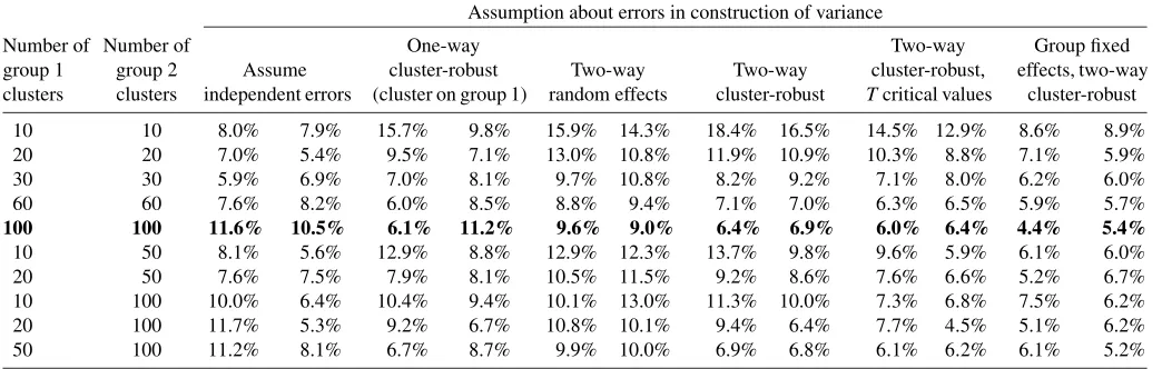
Table 1. Rejection probabilities for a true null hypothesis. True model: a random effect common to each group, and a heteroscedastic component
Assumption about errors in construction of variance
Number of Number of One-way Two-way Group fixed group 1 group 2 Assume cluster-robust Two-way Two-way cluster-robust, effects, two-way clusters clusters independent errors (cluster on group 1) random effects cluster-robust Tcritical values cluster-robust
10 10 8.0% 7.9% 15.7% 9.8% 15.9% 14.3% 18.4% 16.5% 14.5% 12.9% 8.6% 8.9% 20 20 7.0% 5.4% 9.5% 7.1% 13.0% 10.8% 11.9% 10.9% 10.3% 8.8% 7.1% 5.9% 30 30 5.9% 6.9% 7.0% 8.1% 9.7% 10.8% 8.2% 9.2% 7.1% 8.0% 6.2% 6.0% 60 60 7.6% 8.2% 6.0% 8.5% 8.8% 9.4% 7.1% 7.0% 6.3% 6.5% 5.9% 5.7%
100 100 11.6% 10.5% 6.1% 11.2% 9.6% 9.0% 6.4% 6.9% 6.0% 6.4% 4.4% 5.4%
10 50 8.1% 5.6% 12.9% 8.8% 12.9% 12.3% 13.7% 9.8% 9.6% 5.9% 6.1% 6.0% 20 50 7.6% 7.5% 7.9% 8.1% 10.5% 11.5% 9.2% 8.6% 7.6% 6.6% 5.2% 6.7% 10 100 10.0% 6.4% 10.4% 9.4% 10.1% 13.0% 11.3% 10.0% 7.3% 6.8% 7.5% 6.2% 20 100 11.7% 5.3% 9.2% 6.7% 10.8% 10.1% 9.4% 6.4% 7.7% 4.5% 5.1% 6.2% 50 100 11.2% 8.1% 6.7% 8.7% 9.9% 10.0% 6.9% 6.8% 6.1% 6.2% 6.1% 5.2%
NOTE: The null hypothesis should be rejected 5% of the time. Number of monte carlo simulations is 2000.
Table1reports results based on 2000 simulations. This yields a 95% confidence interval of(4.0%, 6.0%)for the Monte Carlo rejection rate, given that the true rejection rate is 5%.
We first consider all but the last two columns of Table 1. The simulations with the largest sample, theG=H=100 row presented in bold in Table 1, confirm expectations. The two-way cluster-robust method performs well. All the other meth-ods, (except the one-way cluster-robust forβ1with clustering on group 1), have rejection rates for one or both ofβ1 andβ2 that exceed 9%. Controlling for one-way clustering on group 1 improves inference on β1, but the tests onβ2then over-reject even more than when iid errors are assumed. The Moulton-type two-way effects method fails when heteroscedasticity is present, with lowest rejection rate in Table1of 8.8% and rejec-tion rates that generally exceed even those assuming iid errors.
The two-way cluster robust standard errors are able to control for both two-way clustering and heteroscedasticity. When stan-dard normal critical values are used there is some over-rejection for small numbers of clusters, but except forG=H=10 the rejection rates are lower than if the Moulton-type correction is used. OnceT critical values are used, the two-way cluster-robust method’s rejection rates are always lower than using the Moulton-type standard errors, and they are always less than 10% except for the smallest design withG=H=10. It is not clear whether the small-sample correction of Bell and McCaf-frey (2002) for the variance of the OLS estimator with one-way clustering, used in Angrist and Lavy (2002) and Cameron, Gel-bach, and Miller (2008), can be adapted to two-way clustering. The final two columns show continued good performance when group specific dummies are additionally included as re-gressors.
Our results are based on the assumption that the group sizeNgh is finite (see theAppendix). However, it does not nec-essarily need to be small compared toGor H. We have esti-mated models similar to this dgp withG=H=30, where we have varied the cell sizes (observations perg×hcell) from 1, as in Table1, to 1000. In these simulations we have also added separate iid N(0,1)errors to each ofx1igh,x2igh, anduigh. Re-sults (not reported) indicate that the two-way robust estimator continues to perform well across the various cell sizes.
We have also examined alternative dgps in which the errors and regressors are distributed iid, and dgps with the classical homoscedastic two-way random-effects design. Results from these simulations can be found in our working paper (Cameron, Gelbach, and Miller2009).
3.2 Monte Carlo Based on Errors Correlated Over Time and States
We now consider an example applicable to panel and re-peated cross-section data, with errors that are correlated over both states and time. Correlation over states at a given point in time may occur, for example, if there are common shocks, while correlation over time for a given state typically decreases with lag length.
We follow Bertrand, Duflo, and Mullainathan (2004) in using actual data, augmented by a variation of their randomly gener-ated “placebo law” policy that produces a regressor correlgener-ated over both states and time. The original data are for 1,358,623 employed women from the 1979–1999 Current Population Sur-veys, with log earnings as the outcome of interest. For each simulation, we randomly draw 50 U.S. states from the original data (and relabel the states from 1 to 50). The model estimated is
yist=αdst+x′istβ+δs+γt+uist, (3.3) whereyist is individual log earnings, the grouping is by state and time (with indicessandtcorresponding togandhin Sec-tion2),dst is a state–year-specific regressor, andxist are indi-vidual characteristics. HereG=50 andH=21 and, unlike in Section3.1, there are many (on average 1294) observations per
(g,h)cell. For some estimations we include state-specific fixed effects δs and time-specific fixed effects γt (69 dummies), as our dgp enables these fixed effects to be identified. In most of their simulations Bertrand, Duflo, and Mullainathan (2004) run regressions on data aggregated into state–year cells. Here we work with the individual-level data in part to demonstrate the feasibility of our methods for large datasets.
Interest lies in inference onα, the coefficient of a randomly assigned “placebo policy” variable. Bertrand, Duflo, and Mul-lainathan (2004) consider one-way clustering, withdst gener-ated to be correlgener-ated within state (i.e., over time for a given state). Here we extend their approach to induce two-way tering, with within-time clustering as well as within-state clus-tering. The placebo law for a state–year cell is generated by
dst=dsst+2d t
st. (3.4)
The variable dsts is a within-state AR(1) variable dsst = 0.6dsts−1+vsst, with vsst iid N[0,1], and is generated
inde-pendently from all other variables. dsst is independent across states. Similarly, the variabledtst is a within-year AR(1) vari-able,dtst=0.6dts−1,t+vtst, correlated over states, with vtst iid
N[0,1], and also independent from other variables. Here the index s ranges from 1–50 based on the order that the states were drawn from the original data. This law is the same for all individuals within a state–year cell. This dgp ensures that dst andds′t′ are dependent if and only if at least one ofs=s′ ort=t′ holds. Because we draw the full time-series for each state, the outcome variables (and hence the errors) are auto-correlated over time within a state. We also add in a wage shockynewist =yoriginalist +0.01wtst, withwtstgenerated similarly to (but independent of)dtst, that is correlated over states. In each of 2000 simulations we draw the 50 states’ worth of individual data, wages are adjusted withwtst, the variabledstis randomly generated, model (3.3) is estimated, and the null hypothesis that
α=0 is rejected at significance level 0.05 if|α|/se[α]>1.96. Given the design used here,αis consistent, and the correct as-ymptotic rejection rates for the simulation results in Table 2
will be 5%, provided that a consistent estimate of the standard error is used.
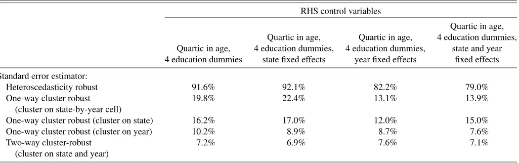
The first column of Table2considers regression ondst and individual controls (a quartic in age and four education dum-mies, without the fixed effectsδsandγt). Since log earningsyist are correlated over both time and state anddstis a generated re-gressor uncorrelated withyist, the erroruist is correlated over both time and state. Using heteroscedastic-robust standard er-rors leads to a very large rejection rate(92%) due to failure to control for clustering. The standard one-way cluster-robust
cluster methods partly mitigate this, though the rejection rates still exceed 19%. Clustering on the 50 states does better than clustering on the 1050 state–year cells. Clustering on year also shows improvements over clustering on state–year cells. We present results from the two-way cluster-robust method in the last row. The two-way variance estimator does best, with rejec-tion rate of 7.2%. This rate is still higher than 5%, in part due to use of critical values from asymptotic theory. Assuming a T(H−1)distribution, withH=21 the rejection rate should be 6.4% (since Pr[|t|>1.96|t∼T(20)] =0.064), and with 1000 simulations a 95% confidence interval is(4.9%, 7.9%). The dgp studied here thus might be well approximated by aT(H−1)
distribution.
For the second column of Table2, we add state fixed effects. The inclusion of state fixed effects does not improve rejec-tion rates for heteroscedasticity robust, clustering on state–year cells, or clustering on state. Clustering on year does somewhat better. As in the first column, two-way robust clustering does best, with rejection rates of 6.9%.
For the third column of Table2, we add year (but not state) fixed effects. In this setting the results for clustering on state-by-year and for clustering on state improve markedly. However, when clustering on state we still reject 12% of the time, which is not close to the two-way cluster robust rejection rate of 7.6%. In column four we include both year and state dummies as re-gressors. For the models using heteroscedastic-robust standard errors the rejection rate is 79%. Clustering on just state–year cells results in rejection rates of 13.9%, which is similar to those from clustering on state (15%). As before, two-way clustering does best, with rejection rates of 7.1%. In this example the two-way cluster-robust method works well regardless of whether or not state and year fixed effects are included as regressors, and gives the best results of the methods considered.
4. EMPIRICAL EXAMPLES
In this section we contrast results obtained using conven-tional one-way cluster-robust standard errors to those using our method that controls for two-way (or multiway) clustering. The
Table 2. Rejection probabilities for a true null hypothesis. Monte Carlos with micro (CPS) data
RHS control variables
Quartic in age, Quartic in age, Quartic in age, 4 education dummies, Quartic in age, 4 education dummies, 4 education dummies, state and year 4 education dummies state fixed effects year fixed effects fixed effects
Standard error estimator:
Heteroscedasticity robust 91.6% 92.1% 82.2% 79.0% One-way cluster robust 19.8% 22.4% 13.1% 13.9%
(cluster on state-by-year cell)
One-way cluster robust (cluster on state) 16.2% 17.0% 12.0% 15.0% One-way cluster robust (cluster on year) 10.2% 8.9% 8.7% 7.6% Two-way cluster-robust 7.2% 6.9% 7.6% 7.1%
(cluster on state and year)
NOTE: Data come from 1.3 million employed women from the 1979–1999 March CPS. Table reports rejection rates for testing a (true) null hypothesis of zero on the coefficient of fake treatments. The “treatments” are generated as (t=es+2et), withesa state-specific autoregressive component andeta year-specific “spatial” autoregressive component. The outcome is
also modified by an independent year-specific autoregressive component. See text for details. 2000 Monte Carlo replications.
first and third examples consider two-way clustering in a cross-section setting. The second considers a rotating panel, and con-siders probit estimation in addition to OLS.
We compare computed standard errors and p-values across various methods. In contrast to the Section3simulations, there is no benchmark for the rejection rates.
4.1 Hersch—Cross-Section With Two-Way Clustering
We consider a cross-section study of wages with clustering at both the industry and occupation level. We base our application on Hersch’s (1998) study of compensating wage differentials. Using industry and occupation injury rates merged into CPS data, Hersch examines the relationship between injury risk and wages for men and women. In this example there are 5960 in-dividuals in 211 industries and 387 occupations. The model is
yigh=α+x′ighβ+γ×rindig+δ×roccih+uigh, (4.1) where yigh is individual log-wage rate, xigh includes individ-ual characteristics such as education, race, and union status, rindig is the injury rate for individual i’s industry androccih is the injury rate for occupation. In this application, as in many similar applications, it is not possible to include industry and occupation fixed effects, because then the coefficients of the key regressorsrindandrocccannot be identified. Hersch em-phasizes the importance of using cluster-robust standard errors, noting that they are considerably larger than heteroscedastic-robust standard errors. She is able to control only for one source of clustering—industry or occupation—and not both simultane-ously.
We replicate results for column 4 of panel B of table 1 of Hersch (1998), with bothrindandroccincluded as regressors. We report several estimated standard errors: default standard er-rors assuming iid erer-rors, White heteroscedastic-robust, one-way cluster-robust by industry, one-way cluster-robust by occupa-tion, and our preferred two-way cluster-robust with clustering on both industry and occupation. We also present (in brackets) p-values from a test of each coefficient being equal to zero.
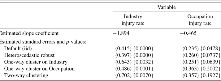
The first results given in our Table3show that heteroscedas-tic-robust standard errors differ little from standard errors based on the assumption of iid errors. The big change arises when clustering is appropriately accounted for. One-way cluster-robust standard errors with clustering on industry lead to sub-stantially larger standard errors for rind (0.643 compared to
0.397 for heteroscedastic-robust), though clustering on industry has little effect on those forrocc. One-way cluster-robust stan-dard errors with clustering on occupation yield substantially larger standard errors forrocc (0.363 compared to 0.260 for heteroscedastic-robust), with a lesser effect for those forrind. In this application it is it is most important to cluster on industry forrind, and to cluster on occupation forrocc.
Our two-way cluster-robust method permits clustering on both industry and occupation. Forrind, the two-way cluster-robust standard error is 10% larger than that based on one-way clustering at the industry level, and is 45% larger than that based on one-way clustering on occupation. Thep-value for a test of zero on the coefficient onrindgoes from 0.0001 (when cluster-ing on Occupation) to 0.0070. Forrocc, the two-way standard error is little different from that based on clustering on occu-pation, but it is 40% larger than that based on clustering on in-dustry. Thep-value on a similar test forroccgoes from 0.0639 (when clustering on Industry) to 0.1927.
4.2 Rose and Engel—Bilateral Trade Model
A common setting for two-way clustering is paired or dyadic data, such as that on trade flows between pairs of countries. Cameron and Golotvina (2005) show the importance of con-trolling for two-way clustering, and propose FGLS estimation based on the assumption of iid country random effects. Here we instead apply our more robust method to an example in their ar-ticle, which replicates the fitted model given in the first column of table 3 of Rose and Engel (2002).
The data are a single cross-section on trade flows between 98 countries with 3262 unique country pairs. A gravity model is fitted for the natural logarithm of bilateral trade. The coeffi-cient of the log product of real GDP (estimated slope=0.867) has heteroscedastic-robust standard error of 0.013, reported by Rose and Engel (2002), and average one-way clustered stan-dard error of 0.031, where we average the one-way standard error with clustering on the first country in the country pair and the one-way standard error clustering on the second country in the country pair. Using the methods proposed in this article, the two-way robust standard error is 0.043. This is 36% larger than the average one-way cluster robust standard error, and 230% larger than the White robust standard error. Note that if country specific effects are included (for each of the two countries in
Table 3. Replication of Hersch (1998)
Variable
Industry Occupation injury rate injury rate
Estimated slope coefficient −1.894 −0.465
Estimated standard errors andp-values:
Default (iid) (0.415) {0.0000} (0.235) {0.0478} Heteroscedastic robust (0.397) {0.0000} (0.260) {0.0737} One-way cluster on Industry (0.643) {0.0032} (0.251) {0.0639} One-way cluster on Occupation (0.486) {0.0001} (0.363) {0.2002} Two-way clustering (0.702) {0.0070} (0.357) {0.1927}
NOTE: Replication of Hersch (1998, p. 604, table 3, panel B, column 4). Standard errors in parentheses.p-values from a test of each coefficient equal to zero in brackets. Data are 5960 observations on working men from the Current Population Survey. Both columns come from the same regression. There are 211 industries and 387 occupations in the data set.
the country pair) as a possible way to control for the clustering, then the coefficient of the log product of real GDP is no longer identified.
For the coefficient on log distance (estimated slope = −1.367), we obtain standard errors of 0.035 (heteroscedastic robust), 0.078 (average of one-way clustered standard errors), and 0.106 (two-way robust). Roughly similar proportionate in-creases in the standard errors are obtained for the coefficients of the other regressors in the model. Allowing for two-way robust clustering impacts the estimated standard errors by a consider-able magnitude.
4.3 Other Examples
We have also examined the importance of clustering in the context of CPS rotating panel design. In an applicaion based on Gruber and Madrian’s (1995) study of health insurance avail-ability and retirement, we examine the importance of cluster-ing on state–year cell (359 clusters) and by household (26,383 clusters). In this particular application the impact of two-way clustering is modest compared to clustering at either level. For more details see Cameron, Gelbach, and Miller (2009).
Foote (2007) reinvestigated Shimer’s (2001) influential find-ing of a (surprisfind-ing) negative correlation between a U.S. state’s annual unemployment rate (dependent variable) and the share of the state’s labor force that is young. Even with relatively high migration by the young, a state’s youth share is highly autocor-related over time; correlation in regional socioeconomic con-ditions also imply that youth shares will be correlated across states within year. Similar two-way correlation is expected for residual state-level unemployment rates.
In the subset of his results that exactly replicates Shimer’s OLS specification [panel A, column (1) of his table I], Foote finds that clustering at the state level, which most researchers likely would do in the wake of Bertrand, Duflo, and Mul-lainathan (2004), raises the estimated standard error from 0.18 to 0.39. Using our method to cluster at both the state and year levels yields as dramatic an increase in the estimated standard error from 0.39 to 0.61, even with state and year fixed effects included as regressors. Clustering on year alone, which would be an uncommon approach, yields a 0.50 estimate. A qualita-tively similar pattern of changes in estimated standard errors is obtained for a specification that instruments the state’s youth share (Foote’s panel B).
5. CONCLUSION
There are many empirical applications where a researcher needs to make statistical inference controlling for clustering in errors in multiple nonnested dimensions, under less restrictive assumptions than those of a multiway random effects model. In this article we offer a simple procedure that allows researchers to do this.
Our two-way or multiway cluster-robust procedure is straightforward to implement. As a small-sample correction we propose adjustments to both standard errors and Wald test crit-ical values that are analogous to those often used in the case of one-way cluster-robust inference. Then inference appears to be reasonably accurate except in the smallest design with 10 clusters in each dimension.
In a variety of Monte Carlo experiments and replications, we find that accounting for multiway clustering can have impor-tant quantitative impacts on the estimated standard errors and associatedp-values. For perspective we note that if our method leads to an increase of 20% in the reported standard errors, then at-statistic of 1.96 with ap-value of 0.050 becomes at-statistic of 1.63 with ap-value of 0.103. Even modest changes in stan-dard errors can have large effects on statistical inference.
The impact of controlling for multiway clustering is great-est when the errors are correlated over two or more dimensions and, in addition, the regressors of interest are correlated over the same dimensions. This is especially likely to be the case when the research design precludes fixed effects along each of the dimensions, as in the Hersch (1998) example. The Hersch ex-ample also illustrates that even if the regressor is most clearly correlated over only one dimension, controlling for error cor-relation in the second dimension can also make a difference. However, we also note that in some settings the impact of the method is modest.
In general a researcher will not know ex ante how important it is to allow for multiway clustering, just as in the one-way case. Our method provides a way to control for multiway clustering that is a simple extension of established methods for one-way clustering, and it should be of considerable use to applied re-searchers.
APPENDIX
We present results for the general case of GMM estimation. Estimation is based on the moment condition E[zi(θ0)] =0for observation i, whereθ is aq×1 parameter vectorθ andzis anm×1 vector withm≥q. Examples include OLS withzi=
(yi−x′iβ)xi, linear IV withzi=(yi−x′iβ)wiwherewiare in-struments forxi, and the logit MLE withzi=(yi−(x′iβ))x′iβ. For models with m=q, such as OLS, logit, and just-identified IV we need only use the m-estimatorθ that solves N
i=1zi(θ)=0. Given two-way clustering with typical cluster
(g,h),zi(θ)=zigh(θ)and N
i=1 zi(θ)=
G
g=1 H
h=1
i∈Cgh
zigh(θ)
=
G
g=1 H
h=1
zgh(θ), (A.1)
whereCghdenotes the observations in cluster(g,h), and
zgh(θ)=
i∈Cgh
zigh(θ) (A.2)
combines observations in cluster(g,h).
For models withm>q, the more general GMM estimatorθ
maximizes Q(θ) = (N−1Ni=1zi(θ))′ W(N−1iN=1zi(θ)), whereW is an m×mfull rank symmetric weighting matrix withW→p W0. The GMM estimator reduces to the m-estimator whenm=q, for any choice ofW.
We assume thatθ is consistent for θ0, that G→ ∞ and H→ ∞at the same rate, so thatG/H → constant, and that the numberNghof observations in cluster(g,h)is not growing
withGorH. Note thatNgh=1 is possible. As discussed below, we consider a rate of convergence√G, so that
√
We now simplifyB0under the assumption of two-way clus-tering. Sinceizi(θ)=ghzgh(θ)we have
where the first triple sum uses dependence if g=g′, the sec-ond triple sum uses dependence ifh=h′, and the third double sum subtracts terms wheng=g′andh=h′which are double counted as they appear in both of the first two sums.
Consider the first triple sum which hasGH2terms. Each of the cross-product termszghz′gh′= bounded away from zero and bounded from above. Then E[zghz′gh′] is bounded, given Ngh fixed, and G−1H−2ghh′E[zghz′gh′] is bounded. Similarly for the second term. The third term has onlyGH terms so this third term goes to zero.
The above analysis assumes that E[zigh(θ)zjgh′(θ)]is boun-ded away from zero. This will be the case for common shocks such as the standard two-way random effects model. But it need not always be the case. As an extreme example, suppose Ngh=1 and that there is no clustering; that is, each observation is independent. Then E[zghz′gh′] =0 unless h=h′ and so the first sum has onlyGHnonzero terms, and similarly for the other two terms. The triple sum is of orderGH, rather thanGH2, and the rate of convergence of the estimator becomes a faster√GH rather than√G. This is the rate expected for estimation based onGHindependent observations.
More generally the triple sum is of order GH, rather than GH2, if the dependence of observations in common clusterg goes to zero as clustershandh′become further apart, as is the
case with declining time series dependence or spatial depen-dence. Then inB0we normalize by(GH)and the rate of con-vergence of the estimator becomes a faster √GH rather than
√
G. Regardless of the rate of convergence, however, we obtain the same asymptotic variance matrix forβ.
Qualitatively similar differences in rates of convergence are obtained by Hansen (2007) for the standard one-way cluster-robust variance matrix estimator for panel data. WhenN→ ∞ withT fixed (a short panel), the rate of convergence is √N. When bothN→ ∞andT→ ∞(a long panel), the rate of con-vergence is√Nif there is no mixing (his theorem 2) and√NT if there is mixing (his theorem 3). While the rates of conver-gence differ in the two cases, he obtains the same asymptotic variance for the OLS estimator.
ACKNOWLEDGMENTS
This article has benefitted from comments from the Editor, an Associate Editor, and two referees, and from presentations at The Australian National University, U.C. Berkeley, U.C. River-side, Dartmouth College, MIT, PPIC, and Stanford University. Miller gratefully acknowledges funding from the National In-stitute on Aging, through grant number T32-AG00186 to the NBER. We thank Marianne Bertrand, Esther Duflo, Sendhil Mullainathan, and Joni Hersch for assisting us in replicating their data sets. We thank Peter Hansen, David Neumark, and Mitchell Petersen for helpful comments, particularly for refer-ring us to relevant literature.
[Received June 2007. Revised May 2009.]
REFERENCES
Acemoglu, D., and Pischke, J.-S. (2003), “Minimum Wages and On-the-Job Training,”Research in Labor Economics, 22, 159–202. [239]
Angrist, J. D., and Lavy, V. (2002), “The Effect of High School Matriculation Awards: Evidence From Randomized Trials,” Working Paper 9389, NBER. [244]
Arellano, M. (1987), “Computing Robust Standard Errors for Within-Group Estimators,”Oxford Bulletin of Economics and Statistics, 49, 431–434. [238,240]
Baughman, R., and Smith, K. (2007), “The Labor Market for Direct Care Work-ers,” Working Paper 07-4, New England Public Policy Center, Federal Re-serve Bank of Boston. [239]
Beck, T., Demirguc-Kunt, A., Laeven, L., and Levine, R. (2008), “Finance, Firm Size, and Growth,”Journal of Money, Credit, and Banking, 40, 1379– 1405. [239]
Bell, R. M., and McCaffrey, D. F. (2002), “Bias Reduction in Standard Errors for Linear Regression With Multi-Stage Samples,”Survey Methodology, 28 (2), 169–179. [244]
Bertrand, M., Duflo, E., and Mullainathan, S. (2004), “How Much Should We Trust Differences-in-Differences Estimates?”Quarterly Journal of Eco-nomics, 119, 249–275. [238,240,244,245,247]
Bester, C. A., Conley, T. G., and Hansen, C. B. (2009), “Inference With De-pendent Data Using Cluster Covariance Estimators,” mimeo, University of Chicago Graduate School of Business. [239]
Bhattacharya, D. (2005), “Asymptotic Inference From Multi-Stage Samples,” Journal of Econometrics, 126, 145–171. [239]
Cameron, A. C., and Golotvina, N. (2005), “Estimation of Country-Pair Data Models Controlling for Clustered Errors: With International Trade Applica-tions,” Working Paper 06-13, U.C.–Davis, Economics Dept. [246] Cameron, A. C., and Trivedi, P. K. (2005),Microeconometrics: Methods and
Applications, Cambridge: Cambridge University Press. [238]
Cameron, A. C., Gelbach, J. G., and Miller, D. L. (2008), “Bootstrap-Based Improvements for Inference With Clustered Errors,”Review of Economics and Statistics, 90, 414–427. [241,244]