Full Terms & Conditions of access and use can be found at
http://www.tandfonline.com/action/journalInformation?journalCode=ubes20
Download by: [Universitas Maritim Raja Ali Haji] Date: 11 January 2016, At: 22:18
Journal of Business & Economic Statistics
ISSN: 0735-0015 (Print) 1537-2707 (Online) Journal homepage: http://www.tandfonline.com/loi/ubes20
Likelihood-Based Estimation of Dynamic Panels
With Predetermined Regressors
Enrique Moral-Benito
To cite this article: Enrique Moral-Benito (2013) Likelihood-Based Estimation of Dynamic Panels With Predetermined Regressors, Journal of Business & Economic Statistics, 31:4, 451-472, DOI: 10.1080/07350015.2013.818003
To link to this article: http://dx.doi.org/10.1080/07350015.2013.818003
Accepted author version posted online: 12 Jul 2013.
Submit your article to this journal
Article views: 357
View related articles
Likelihood-Based Estimation of Dynamic Panels
With Predetermined Regressors
Enrique M
ORAL-B
ENITOBanco de Espa ˜na Alcal ´a 48, 28014 Madrid, Spain ([email protected])
This article discusses the likelihood-based estimation of panel data models with individual-specific effects and both lagged dependent variable regressors and additional predetermined explanatory variables. The resulting new estimator, labeled as subsystem limited information maximum likelihood (ssLIML), is asymptotically equivalent to standard panel generalized method of moment asN→ ∞for fixedTbut tends to present smaller biases in finite samples as illustrated in simulation experiments. Simulation results also indicate that the estimator is preferred to other alternatives available in the literature in terms of finite-sample performance. Finally, to provide an empirical illustration, I revisit the evidence on the relationship between income and democracy in a panel of countries using the proposed estimator.
KEY WORDS: Dynamic panel data; Income and democracy; Maximum likelihood estimation; Monte Carlo methods.
1. INTRODUCTION
In this article, I consider a linear panel data model with individual-specific effects and both a lagged dependent variable regressor and additional predetermined explanatory variables. In particular, I develop the implications of the model (without imposing any additional restriction) for the first- and second-order moments of the observed data to set up a likelihood func-tion based on a multivariate regression with normal errors and restrictions on the covariance matrix.
To avoid steady-state restrictions and the incidental param-eter problem, the vector of initial observations and individual effects is assumed to be normally distributed with unrestricted mean and covariance matrix. Also, neither time-series nor con-ditional homoscedasticity are assumed. Therefore, the resulting subsystem limited information maximum likelihood (LIML)— henceforth ssLIML—estimator1 remains consistent under the same assumptions as standard panel generalized method of mo-ment (GMM) estimators (e.g., Arellano and Bond1991).
More concretely, ssLIML is asymptotically equivalent to the standard GMM estimator discussed in Arellano and Bond (1991) augmented with moment conditions implied by the se-rial correlation properties of the errors as suggested by Ahn and Schmidt (1995).2 Along these lines, ssLIML can be
in-This article is a substantially revised version of a previous draft circulated under the title “Dynamic Panels With Predetermined Regressors: Likelihood-based Estimation and Bayesian Averaging With an Application to Cross-Country Growth.” The STATA commandxtmoralbthat implements the estimator dis-cussed in this article is available on my website athttp://www.moralbenito.com.
1Note that the model consists ofTstructural equations for the dependent
vari-able (y) completed with a set of reduced-form equations for the additional predetermined explanatory variables (x) and the initial observations. Therefore, the ssLIML labeling can be understood as an intermediate situation between LIML—a single structural equation and a set of reduced-form equations—and full information maximum likelihood (FIML)—a set of structural equations without reduced-form equations (see Hendry1995).
2More concretely, Ahn and Schmidt (1995) suggested to exploit the moment
conditions resulting from the lack of autocorrelation in the errors available under the assumption of conditional mean independence between the time-varying errors and the individual effects. Note that these moment conditions make the estimation problem nonlinear and, thus, have been generally ignored by applied researchers.
terpreted as the likelihood-based counterpart of method-of-moments estimators for dynamic panels with predetermined regressors.
It is well known from the simultaneous equations literature (e.g., Anderson, Kunitomo, and Sawa 1982) that likelihood-based approaches are preferred to method-of-moments counter-parts in terms of finite-sample performance, especially when the instruments are weak and/or many with respect to the sample size. Therefore, the aforementioned ssLIML estimator is ex-pected to be preferred to its method-of-moments counterpart in terms of finite sample performance.
A comprehensive simulation study serves to evaluate the finite-sample behavior of the ssLIML estimator. In settings with individual effects and both a lagged dependent variable regressor and an additional predetermined explanatory variable, I find that the finite-sample biases of the ssLIML estimator are in general negligible. Moreover, the ssLIML biases tend to be smaller than those of other estimators available in the literature, especially when instruments are expected to be weaker (i.e., the series are more persistent because either the autoregressive parameter is more sizable or a larger variance of the individual effects exists).
This work is related to the literature exploring alternative es-timators that are asymptotically equivalent to standard GMM as
N → ∞for fixedT, but potentially having different finite sam-ple behavior (e.g., Alonso-Borrego and Arellano 1999). This literature is motivated by concern with the finite-sample bi-ases in standard GMM, especially when the instruments are weak and the number of moment conditions is large relative to the cross-section dimension (see, e.g., Blundell and Bond 1998).
© 2013American Statistical Association Journal of Business & Economic Statistics October 2013, Vol. 31, No. 4 DOI:10.1080/07350015.2013.818003 451
Based exclusively on the same identifying assumption as standard GMM (i.e., predeterminedness), Alonso-Borrego and Arellano (1999) considered both LIML analog3and
symmetri-cally normalized GMM estimators, which tend to reduce finite-sample biases in standard GMM. Alternatively, Arellano and Bover (1995) and Blundell and Bond (1998) resorted to auxiliary mean-stationarity assumptions in addition to predeterminedness and exploit them within a method-of-moments perspective in the so-called system GMM (sGMM) estimator.
The present article is also related to the literature on likelihood-based estimation of panel data models under
fixed-T and large-N settings. Bhargava and Sargan (1983), Alvarez and Arellano (2003), and Dhaene and Jochmans (2012), among others, considered likelihood functions for an autoregressive panel data model with strictly exogenous regressors. In con-trast, the likelihood function developed by Hsiao, Pesaran, and Tahmiscioglu (2002) for data in differences can also accommo-date predetermined regressors under the assumption of time-series homoscedasticity of the error variances4 [Alvarez and
Arellano (2004) discussed the relationship of this approach with other maximum likelihood (ML) estimators for the data in levels].
As an empirical illustration, I use the proposed estimator to revisit the evidence on the effect of income on democracy in a panel of countries spanning from 1970 to 2000 with data at 5-year intervals. Based on ordinary least squares (OLS) estimates, Acemoglu et al. (2008) found that the positive correlation be-tween income and democracy disappears when accounting for country-specific effects. Given the potential feedback from in-come to democracy, Acemoglu et al. (2008) also considered the Arellano and Bond (1991) GMM estimator in search of a causal interpretation for their OLS estimates. Based on this GMM estimator, Acemoglu et al. (2008) obtained negative (and often significant) estimates of the effect of income on democ-racy. In contrast, ssLIML estimates are always statistically insignificant.
The remainder of the article is organized as follows. Section2 presents the likelihood function and the connection between the resulting ssLIML estimator and its method-of-moments coun-terpart. Monte Carlo evidence on the finite-sample behavior of the estimator is provided in Section 3. In Section4, I re-visit the evidence on the relationship between income and democracy across countries using the ssLIML estimator. Fi-nally, Section5concludes. Additional results are gathered in the Appendix.
3Sargan (1958) showed that the original LIML estimator (based on a proper
likelihood function) developed by Anderson and Rubin (1949) is equivalent to an IV (instrumental variables)/GMM estimator that minimizes the maximum possible sample correlation between the errors and a linear combination of the instruments. Therefore, in contrast to the ssLIML estimator discussed in this article, “minimax” method-of-moments estimators such as those considered in Alonso-Borrego and Arellano (1999) and Akashi and Kunitomo (2010) are usually labeled as LIML analog estimators in spite of not corresponding to any meaningful ML estimator.
4Binder, Hsiao, and Pesaran (2005) also considered a likelihood approach for
dynamic panel data models with predetermined regressors under time-series homoscedasticity and mean-stationarity.
2. DYNAMIC PANEL DATA WITH FEEDBACK: LIKELIHOOD-BASED ESTIMATION
In addition to being potentially correlated with a time-invariant unobserved heterogeneity component, regressors in panel data models can be assumed to be uncorrelated to past, present, and future time-varying errors (i.e., strictly exogenous) or correlated with time-varying errors at all lags and leads (i.e., strictly endogenous). Besides these two configurations, it is pos-sible to imagine intermediate settings in which the explanatory variables can be correlated with time-varying errors at certain periods but not at others (i.e., partially endogenous).
In this article, I consider a dynamic panel data model in which the time-varying errors are uncorrelated with current and lagged values of the regressors but not to their future values (i.e., regressors are predetermined with respect to the current time-varying error).5
Formally, I consider the model
yit =αyit−1+xit′β+wi′δ+ηi+ζt+vit (1)
Evit |yti−1, x t i, wi, ηi
=0 (t =1, . . . , T)(i=1, . . . , N),
(2)
where xit andwi are vectors of variables of ordersk andm,
respectively, and xit denotes a vector of the observations of
xaccumulated up tot:xti =(x′i1, . . . , xit′)′. I use, with a slight abuse of notation, the subscriptit−1 as a shorthand fori, t−1. Analogously to standard GMM, condition (2) is the only assumption required for consistency and asymptotic normality (under fixedTwhenNtends to infinity) of the likelihood-based estimator developed in this article. Other ML estimators are available in the literature for estimating the model in (1) and (2). However, these estimators require additional assumptions such as time-series homoscedasticity (i.e., Hsiao, Pesaran, and Tahmiscioglu2002) or mean-stationarity (i.e., Binder, Hsiao, and Pesaran2005) for fixed-Tconsistency.
In addition to the predetermined variablesyit−1 andxit, the
model also includes a vector of time-invariant strictly exogenous variables (wi). Allowing for time-varying strictly exogenous
re-gressors is straightforward in this context. However, in the spirit of Hausman and Taylor (1981), I stress here the possibility of identifying the effect of time-invariant observable variables in addition to the unobservable time-invariant fixed effect (ηi) by
assuming lack of correlation between thew variables and the fixed effects. Finally, the termζtin (1) captures unobserved
com-mon factors across units in the panel, and thus, this particular form of cross-sectional dependence is allowed.6
The model in (1) and (2) assumes that both the lagged de-pendent variable and thex regressors are predetermined with respect to the time-varying error term (vit). This configuration
5Since predetermined variables are potentially correlated to lagged values of
the time-varying error but are uncorrelated to present and future values, they can be understood as a particular case of partial endogeneity. For instance, an alternative partial endogeneity setting may also allow for nonzero correlation between the regressor and the contemporaneous time-varying error so that the regressor is no longer predetermined although partially endogenous.
6In practice, this is done by simply working with cross-sectional demeaned
data. In the remainder of the exposition, all of the variables are assumed to be deviations from their cross-sectional mean.
accommodates feedback from lagged values of the dependent variableyto the current value of thexregressors.7It is worth
emphasizing that assumption (2) also implies lack of autocor-relation invit since laggedv’s are linear combinations of the
variables in the conditioning set.
2.1 Likelihood Function With an Unrestricted Feedback Process
In contrast to a model with only strictly exogenous explana-tory variables, the specification of the model in (1) and (2) with predetermined variables is incomplete in the sense that it does not lead to a likelihood in itself once we add an error distri-butional assumption. Therefore, in this section, I develop the implications of the model for the first and second moments of the observed variables. The parameters in Equation (1) are augmented with additional (implicit and unrestricted) reduced-form parameters required for specifying these moments. Once the moments are specified, I can set up a likelihood function based on a multivariate regression model with restrictions on the covariance matrix.
The unrestricted feedback process is specified in the form of a set of cross-sectional linear projections of the predeterminedx
variables on all available lags (fort=2, . . . , T) having period-specific coefficients:
xit =κtwi+γt0yi0+ · · · +γt,t−1yi,t−1
+ t1xi1+ · · · + t,t−1xi,t−1+ctηi+ϑit. (3a)
Furthermore, the mean vector and covariance matrix of the joint distribution of the initial observations (yi0, xi1) and the individual effectsηi are unrestricted. This is in sharp contrast
with the mean-stationarity assumption required by the so-called sGMM estimator discussed in Arellano and Bover (1995) and Blundell and Bond (1998). As a result, I do not impose any stationarity assumption on the initial observations:8
yi0 =w′iδ0+c0ηi+vi0 (3b)
respectively, andϑitis ak×1 vector of prediction errors.
All in all, the full model consists of theT equations in (1) plus theT k+1 equations in (3a)–(3c). The equations of interest (i.e., structural equations) are those corresponding to y. The remaining equations in the system are not of relevant interest and are thus considered as reduced-form equations. Therefore,
7A static (i.e., without lagged dependent variable) version of the model might
also be of interest, for instance, in the estimation of production functions (e.g., Blundell and Bond2000) or Euler equations for household consumption (e.g., Zeldes1989). The likelihood function for such a static version is also discussed in AppendixA.2.
8Note also that this specification implies that cov(η
i, wi)=0 to ensure
identi-fication ofδin (1).
9Note that strict exogeneity of a givenxjregressor can be tested by considering
the nullH0:γt hj =0 for allh < tagainst the alternativeH1:γt hj =0 for at
least oneh < t.
once I set up the corresponding likelihood function, I label the approach as subsystem LIML (ssLIML) as opposed to FIML (all equations in structural form) or LIML (a single structural equation plus a set of reduced-form equations).
To rewrite the system in matrix form, I also define theT(k+
1)+1×1 vector of observed data for individuali:
variance-covariance matrix allows for time-series het-eroscedasticity.
I further define theT(k+1)+1×T(k+1)+1 lower tri-angular matrix of coefficientsBas
B=
I am now able to write the model as
Ri =(θ)′wi+Ui∗ (4) Note thatθ augments the parameters of interest (α, β, δ) from Equation (1) with auxiliary parameters that are unrestricted ex-cept that the variances are positive (i.e.,ση2andσv2t are positive, andϑt is definite positive∀t) so that(θ) is positive definite.
Also, the vech operator here stacks by rows the lower triangle of a square matrix so that we eliminate redundant elements of the
10More specifically, p
covariance matrix due to symmetry (vec operates analogously but stacking by rows the full matrix).
I also define the matrices of dataR =(Y0X1 Y1 . . . XT YT),
Xt=(Xt1, . . . , Xkt), andW =(w1, w2, . . . , wN)′of ordersN×
T(k+1)+1,N×k, andN×m, respectively. Thus, the joint distribution ofRconditional onW is
R|W ∼N(W (θ), IN⊗(θ)) (6)
with log-likelihood
L∝ −N
2 log det(θ)− 1 2tr{(θ)
−1
[R−W (θ)]′
×[R−W (θ)]}, (7)
which depends on a fixed number of parameters and satisfies the usual regularity conditions. Moreover, if the distribution ofRis not assumed to be normal, the maximizer ofLcan be regarded as a Gaussian pseudo ML estimator, which remains consistent and asymptotically normally whenNtends to infinity for fixedT
as shown in Section2.3. Moreover, as also discussed in Section 2.3, this estimator is asymptotically equivalent to the class of first-differenced GMM estimators discussed in Arellano and Bond (1991) augmented with moments resulting from lack of autocorrelation in the errors implied by assumption (2) (see Ahn and Schmidt1995).
This parameterization of the complete model is labeled as Full Covariance Structure (FCS) representation. In this param-eterization, the coefficient matrix Bincludesγt hand t hthat
are the vectors and matrices gathering all the feedback from laggedy’s to currentx’s and the dynamic relationships between the xvariables, respectively. These parameters are not of rel-evant interest in our setting, but, in principle, they also need to be estimated. This might represent a concern since the log-likelihood optimization problem becomes cumbersome given the high dimension ofθ.
However, to satisfy the same number of restrictions imposed by (1) and (2) in the first- and second-order moments of the observed data, there is a one-to-one mapping between the pa-rameters inBand. For instance, the reduced-form parameters inγt hcapture the feedback fromyiin periodhtoxi in periodt
withh < t. In the spirit of the simultaneous equations literature and without imposing any additional restriction, this feedback can also be captured through additional nonzero elements in the variance-covariance matrix , which would no longer be block-diagonal (see below). This mapping also applies to the parameters in t hcapturing the dynamic effects between thex
regressors.
Fully developing this feature, I present in the next section another parameterization [labeled as simultaneous equations model (SEM)] that captures the feedback process and the dy-namic relationships between thex’s in the variance-covariance matrix of the system. This SEM parameterization turns out to be useful in practice because it produces closed-form solutions for some reduced-form parameter estimates. This enables me to concentrate out the parameters of the dynamic relationships between thex’s, which are not of pertinant interest. Given the resulting profile likelihood (described in Appendix A.1), the estimation problem becomes computationally affordable.
2.2 Simultaneous Equations Model (SEM) Representation
In this section, I present an SEM representation that enables me to make the likelihood optimization computationally afford-able. For that purpose, I specify some reduced-form parameters in the variance-covariance matrix so that, given the resulting pa-rameterization, estimates for these parameters have closed-form solutions.
Importantly, consistency and asymptotic normality in the SEM parameterization still rely exclusively on assumption (2). Stationarity assumptions are avoided by considering an unre-stricted mean vector and covariance matrix of the joint distribu-tion of initial observadistribu-tions and individual effects. Also, neither time-series nor conditional homoscedasticity are assumed.
In the spirit of the simultaneous equations literature, the role of the strictly exogenous regressors (i.e., the initial observations
yi0andxi1, and thewi regressors) is placed in the mean vector
of the endogenous variables. For this purpose, I first define the following:
ηi =φ0yi0+xi′1φ1+ǫi, (8)
where the scalarφ0and thek×1 vectorφ1represent parameters to be estimated andǫican be interpreted as an individual-specific
effect uncorrelated with the initial observations.11
Along these lines, I now define the reduced-form equations for thexvariables as follows:
xit =πt0yi0+πt1xi1+πtwwi+ξit (t =2, . . . , T), (9a)
where ξit and πt0 are k×1 vectors of prediction errors and coefficients, respectively;πt1is ak×kmatrix andπtwak×m
matrix.
Moreover, by substituting (8) in (1),
yit =αyi,t−1+xit′β+φ0yi0+xi′1φ1+w′iδ+ǫi+vit
(t=1, . . . , T). (9b)
Note that the set of equations in (9a) only includes as right-hand side variables the initial observations [which can be con-sidered as strictly exogenous according to assumption (2)] and the strictly exogenous regressorsw. Therefore, reduced-form equations in (9a) no longer include either the feedback process or the dynamic relationships between thex’s. These relation-ships will be captured in the variance-covariance matrix of the model, as discussed below.
To write the system in a matrix form convenient for concen-tration of the reduced-form parameters, I define the following
T +(T −1)k×1 vectors of data and errors for individuali:
˜
Ri =(yi1, yi2, . . . , yiT, xi′2, xi′3, . . . , x′iT)′
˜
Ui =(ǫi+vi1, . . . , ǫi+viT, ξi′2, . . . , ξiT′ )′.
Therefore, the model can be written in matrix form as
˜
BR˜i=Cz˜ i+U˜i, (10)
11Note that another possibility would be to set the parameters capturing the
correlation between the effects and the initial observations (φ0, φ1) in the ˜12
matrix below. Note also that in (8), I am implicitly assuming that cov(ηi, wi)=0
to ensure identification ofδ.
where ˜Band ˜C are matrices of coefficients defined below and
ziis the (1+k+m)×1 vector of strictly exogenous variables:
zi =(yi0, xi′1, wi′)′.
Moreover, if we additionally define the following vectors
˜
Ri1=(yi1, yi2, . . . , yiT)′ R˜i2=(xi′2, xi′3, . . . , xiT′ )′
˜
Ui1 =(ǫi+vi1, . . . , ǫi+viT)′ U˜i2 =(ξi′2, . . . , ξiT′ )′,
it is then possible to rewrite
In contrast to the FCS representation, in the SEM parameter-ization, the number of nonzero coefficients in the matrix ˜B is onlyk+1. This is so because the feedback process parameters together with the parameters capturing the dynamic relation-ships between thex’s regressors have been “translated” into the variance-covariance matrix of the model, which is no longer block-diagonal.12
12Note also that the matrixπw
t contains the parameters capturing the effect
ofwi onxit, and it is therefore the equivalent to theκt matrix in the FCS
parameterization.
where
1. ˜11has the classical error-component form but allowing for time-series heteroscedasticity: ers all of the contemporaneous and dynamic relationships between thexvariables:
where t,h is thek×kcovariance matrix betweenξit and
ξihfort =2, . . . , T andh=2, . . . T. Note that the effects
captured through parameters in ˜22 andπt1were captured through t h(withh < t) andϑt in the FCS
parameteriza-tion in Secparameteriza-tion2.1.
3. ˜12 captures the feedback process. In particular, given the assumptions above fort=2, . . . , T, we can write
Note here that theψt h (forh < t) parameters together with
πt0capturing the feedback process in the SEM parameterization are equivalent to theγt h(forh < t) parameters in the FCS
pa-rameterization. Also, theφtvectors of parameters are equivalent
to thect vectors in the FCS parameterization fort =0, . . . , T.
Rearranging (10), we have ˜
13Other partial endogeneity configurations can also be accommodated in
ad-dition to the baseline predeterminedness assumption in (13a) and (13b). For example, allowing for nonzero correlations betweenxitand contemporaneous
shocks (vit) is straightforward by considering cov(vih, ξit)=ψt hifh≤t
in-stead of (13b).
The joint distribution of ˜Rconditional onZcan be written as
˜
R|Z∼NZ˜( ˜θ), IN⊗˜( ˜θ)
(16)
with the resulting log-likelihood14
˜
row vectors of each of theNunits in the panel.
As in the case of the FCS representation, the maximizer of ˜L
is a consistent and asymptotically normal estimator regardless of nonnormality. The resulting (pseudo) ML estimator is asymp-totically equivalent to the GMM estimator discussed in Arellano and Bond (1991) augmented with the moments discussed in Ahn and Schmidt (1995) given by the lack of autocorrelation in the errors.
Finally, given the SEM parameterization, some reduced-form coefficients in ˜θhave closed-form solution. Thus, the dimension of the problem can be drastically reduced if we consider the profile likelihood as described in AppendixA.1.
2.3 Asymptotic Normality and Relationship With Method-of-Moments Estimators
Without considering strictly exogenous variables (w) for the ease of exposition, the model in Equations (1) and (2) implies the following first- and second-order moments of the observed data as discussed in the previous sections:15
E(Ri)=0 (18)
E(RiRi′)=(θ), (19)
where 0 is a T(k+1)+1×1 vector of zeros and Ri and
(θ) are defined above. Instead of a likelihood-based approach, one can also consider the following moment conditions to estimateθ:
vechE[RiRi′−(θ)]=E[si−ω(θ)] (20)
and proceed within a GMM framework provided that standard identification conditions hold
consistent estimator of the covariance matrixV =var(si).
In particular, the focus here is on GMM estimators based on the optimal weighting matrix under normality ˆV−1
=
this type can be reformulated in terms of transformations of the original moments in (20) (see Arellano2003, p. 70); hence, the GMM estimator in (21) belongs to the class of one-step estimators discussed in Arellano and Bond (1991) augmented
14Since det( ˜B)=1 and given the properties of the trace of a product of matrices,
the likelihood can also be expressed as ˜L∝ −N2 log det( ˜)− 1
2tr( ˜−1U˜′U˜). 15Note that the variables are expressed in deviations from their cross-sectional
mean to consider time effects.
with the Ahn and Schmidt (1995) quadratic moment restrictions given by the lack of autocorrelation of the errors implied by as-sumption (2). Indeed, the number of overidentifying restrictions (q−p) imposed by this GMM estimator coincides with the number of restrictions imposed in the covariance matrix by the pseudo ML estimator (ssLIML). For instance, ifT =3,k=1, andm=0, the aforementioned GMM estimator exploits seven moment conditions for estimating two parameters and thus im-posing 7−2=5 overidentifying restrictions; in the case of the ssLIML estimator, ifT =3,k=1, andm=0, the unrestricted covariance matrixincludes (7×8)/2=28 parameters to be estimated, while the restricted version in (5) only contains 23 parameters implying 28−23=5 overidentifying restrictions.
The first-order conditions from the problem in (21) are
−
and the resulting estimator can be proved to be consistent and asymptotically normal within the class of GMM estimators.16
In contrast, the pseudo ML estimator (ssLIML) discussed in this article solves
The first-order conditions resulting from this problem are given by
The first-order conditions in (24) have the same form as those of the GMM problem in Equation (22). The only difference arises due to the (continuously updated) weighting matrix im-plicitly used by the optimization problem in (23). Therefore, the asymptotic distribution of both estimators ˆθssLIMLand ˆθGMMis the same with or without normality.
To formally establish this equivalence together with the explicit formula of the asymptotic variance-covariance matrix, I elaborate a restatement of the results in Section 4.4 of Chamberlain (1984). In particular, the following assumptions will be imposed throughout:
1. ⊂Rpis an open set containingθ.
2. ωis a continuous, one-to-one mapping ofintoRq with a
continuous inverse.
3. ωhas continuous second partial derivatives in. 4. rank[∂ω∂c(c′)]=pforc∈.
5. (c) is nonsingular forc∈.
6. √N(¯s−ω(θ))→D N(0,V), where V=var(Ri⊗Ri) and
¯
s→a.s.ω(θ).
Theorem 1. Let Assumptions 1–6 hold. Then, for fixed T
as N → ∞, √N( ˆθssLIML−θ) has the same limiting
distri-16See Chamberlain (1982) and Abowd and Card (1989) for detailed analyses on
the estimation and testing of covariance structures from panel data.
Proof. See propositions 2 and 5 in Chamberlain (1984).17
Theorem 1 states the asymptotic equivalence between ˆθssLIML and ˆθGMM together with the common asymptotic variance-covariance matrix. If the distribution ofRi is normal,Wis the
minimal variance-covariance matrix within this class of estima-tors (see Richard1975). Under nonnormality both estimators remain consistent and asymptotically normal but they are in-efficient for large-N relative to an alternative GMM estimator based on ˆV = N1 Ni=1sisi′−ss¯′.
3. MONTE CARLO EVIDENCE
In this section, I investigate the finite sample behavior of the ssLIML estimator in relation to other available alternatives for estimating panel data models with both lagged dependent variable regressors and additional predetermined explanatory variables correlated with the individual effects. For this purpose, I closely follow the simulation setting in Bun and Kiviet (2006).
3.1 Data-Generating Process
I generate the simulated samples from a panel data model with a lagged dependent variable, individual effects, and an-other (potentially predetermined) explanatory variable. More specifically, data for the dependent variableyand the explana-tory variablexare generated according to the following:
yit =αyit−1+βxit+ηi+vit (25)
xit =ρxit−1+φyit−1+π ηi+ξit, (26)
where vit,ξit, and ηi are generated asvit ∼iid(0, σv2), ξit ∼
iid(0, σξ2), andηi ∼iid(0, ση2), respectively. The parameterφin
(26) captures the feedback from the lagged dependent variable to the regressor so thatxis strictly exogenous ifφ=0.
This particular data-generating process (DGP) corresponds to scheme 2 in Bun and Kiviet (2006).18 With respect to the
parameter values, I consider all of the feasible designs in Bun and Kiviet (2006). In particular, the parameter values explored include α= {0.25,0.75}, β =1−α, ρ= {0.50,0.95}, φ=
[φ1(1−α)(1−ρ)]/[1+βφ1] with φ1 = {−1,0,1}, and π = π1(1−ρ−φ)−φ/(1−α) withπ1= {−1,0,1}. The variance of the disturbance termσ2
v is normalized to 1, and the variance
of the individual effects (σ2
η) is fixed such that the impact of
the two variance componentsηi andvit on the variance ofyit
has a ratioμ2 with μ= {0,1,5}. Finally, for the regressor’s disturbance (σξ2), I consider the signal-to-noise ratio (ζ), which determines the usefulness ofxit for explainingyit and is fixed
to be either 3 or 9 in the simulations. Bun and Kiviet (2006) provided more details about this choice of parameter values, which covers a wide range of configurations.
The resulting combinations of parameter values are such that the processes fory andx are both stable but not necessarily stationary. Bun and Kiviet (2006) only considered stationarity
17Note that since ¯sis a sample average, ˆθ
GMMis both a GMM and a minimum
distance estimator in the terminology of Chamberlain (1984).
18I consider this scheme because, as acknowledged by Bun and Kiviet (2006),
it is more realistic than their baseline scheme 1, considered for convenience in the evaluation of their analytical results.
settings by additionally assuming that both processes started in the distant past. Equivalently, stationarity can also be achieved by imposing that the distribution of the initial observations coin-cides with the steady-state distribution. In particular, stationarity in mean requires that the mean of the initial observation condi-tional on the individual effects coincides with the steady-state mean. Since I generate the initial observations according to
yi0=πy0ηi+vi0 (27) xi0=πx0ηi+ξi0, (28) mean-stationarity can be achieved by imposing
πy0=
βπ+(1−ρ)
(1−ρ)(1−α)−βφ (29)
πx0=
φ+π(1−α)
(1−ρ)(1−α)−βφ (30)
while the processes can be mean-nonstationary provided πy0 andπx0are left unrestricted.
Allowing for mean-nonstationarity may be desirable in many empirical applications. For instance, when analyzing cross-country datasets starting at the end of a war (or micro panels for young workers or new firms), initial conditions at the start of the sample may not be representative of the steady-state behavior of the different processes, and thus mean-stationarity may not hold. Therefore, in contrast to Bun and Kiviet (2006), I also consider the case of mean-nonstationarity in the simulations.
3.2 Estimators
In addition to the ssLIML estimator discussed in Section2, the performance of seven competing estimators is evaluated in the simulations.
Note that Equation (25) can be rewritten as
yit =h′itb+ηi+vit (31)
withhit =(yit−1, xit) andb=(α, β)′.
The standard assumption considered throughout the article [see Equation (2)] is given by
Evit|hti, ηi
=0. (32)
Under assumption (32), the following set of linear moment conditions is available:19
Ehti−1(yit∗ −h∗it′b)=0. (33) Based on these orthogonality conditions, I first consider the well-known first-differenced GMM estimator (e.g., Arellano and Bond1991), which solves
ˆ
bGMM=arg min
b
(y∗−H∗b)′ZANZ′(y∗−H∗b), (34)
where y∗
i =(yi1, . . . , yi,T−1)′, h∗i =(h′i1, . . . , h′i,T−1)′, y∗= (y∗′
1, . . . , y∗
′
N)′, H∗=(h∗
′
1, . . . , h∗
′
N)′, and Z=(Z1′, . . . , ZN′ )′.
Zi is a block diagonal matrix whose tth block is hti−1. In
particular, I consider the one-step nonrobust weighting matrix
AN ∝(Z′Z)−1.
19Starred variables denote forward orthogonal deviations (see Arellano and
Bover1995).
Since ˆbGMMis expected to have poor finite-sample properties [see for instance Blundell and Bond (1998)], I also consider two asymptotically equivalent alternatives that may have differ-ent finite-sample properties. First, the symmetrically normalized GMM estimator (henceforth SNM) proposed in Alonso-Borrego and Arellano (1999) exploits the vector of orthogonality condi-tions in (33) but normalized to have unit length:
ˆ
bSNM=arg min
b
(y∗−H∗b)′ZANZ′(y∗−H∗b)
1+b′b . (35)
Second, LIML analog estimators (e.g., Alonso-Borrego and Arellano1999; Akashi and Kunitomo2010), or “continuously updated GMM” in the terminology of Hansen, Heaton, and Yaron (1996), minimize the maximum possible sample correla-tion between the errors and the instruments according to moment conditions in (33). In particular, we consider in our simulation study a nonrobust LIML analogue that minimizes a criterion of the form
ˆ
bLIML=arg min
b
(y∗−H∗b)′ZAN(b)Z′(y∗−H∗b), (36)
whereAN(b)=(Z′Z)−1/(y∗−H∗b)′(y∗−H∗b).
The estimators ˆbGMM, ˆbSNM, and ˆbLIMLare all based on the same moment conditions in (33) and have the same asymptotic distribution asN → ∞for fixedT (see Alonso-Borrego and Arellano1999for more details). However, they are expected to have different sampling behavior mainly because of the alterna-tive normalization rules adopted in the three cases (see Hillier 1990).
As suggested by Ahn and Schmidt (1995), henceforth AHNS, in addition to the orthogonality conditions in (33), we can also consider the following moment conditions given the lack of serial correlation in the errors implied by (32):
E[vi,t−1(yit−hit′b)]=0 (t=3, . . . , T) (37)
and exploit them within the standard GMM framework above. The resulting GMM estimator, labeled here as ˆbAHNS, mini-mizes a criterion such as the one in (34) but also using lagged first-differenced errors as instruments for the errors in levels. Note that the GMM estimation problem becomes nonlinear in this case.
The ssLIML estimator ( ˆbssLIML) proposed in this article im-plicitly considers these additional moment conditions, and it can be shown to be asymptotically equivalent to ˆbAHNSasN → ∞ for fixedT(see Section2.3).
In addition to the baseline assumption in (32), one can also assume that the processes for y and x are mean-stationary. Mean-stationarity implies thatE(yit|ηi) andE(xit|ηi) are
time-invariant so that changes inyit orxitare mean independent of
the individual effectηi:
E(yit−yi,t−1|ηi)=0 (38)
E(xit−xi,t−1|ηi)=0. (39)
If we are willing to consider this mean-stationarity assump-tion, we can also exploit the resulting moment conditions as discussed in Arellano and Bover (1995). In particular, under as-sumptions (38) and (39), first differences of the right-hand-side
variables can be used as instruments for the errors in levels:
E[hit(yit−h′itb)]=0 (t =3, . . . , T). (40)
As a result, the so-called sGMM estimator ( ˆbsGMM) solves the minimization problem in (34) using the combined set of moments in (40) and (33) and the matrices of data and instru-ments defined accordingly [see Arellano and Bover (1995) for more details].
The sGMM estimator is also included in the simulation given its popularity in applied research. However, it is worth emphasizing that the remaining estimators considered (i.e., GMM, SNM, LIML, AHNS, and ssLIML) are consistent under nonstationarity while they remain consistent under mean-stationarity. In contrast, sGMM requires mean-stationarity (which might not hold in many empirical applications) for con-sistency.
Finally, the ML estimator in first differences suggested in Hsiao, Pesaran, and Tahmiscioglu (2002) is also included in the simulation exercise. In particular, this estimator (labeled as
ˆ
bHPT) solves
ˆ
bHPT=arg min
b
N
2 ln det §
+1
2
N
i=1
u§i′§u§i, (41)
where§ andu§i are given by equations (3.2) and (4.16) in Hsiao, Pesaran, and Tahmiscioglu (2002). Note that, in contrast to the remaining estimators considered here (i.e., GMM, SNM, LIML, AHNS, ssLIML, and sGMM), ˆbHPTwill be inconsistent for fixed T as N → ∞ if the unconditional variances of the errors vary over time.
For the sake of completeness, we also consider the within-group or least-squares dummy-variable (henceforth LSDV) es-timator which is given by the slope coefficients in an OLS regression ofyitonhitand a full set of individual dummy
vari-ables, or equivalently by the OLS estimate in deviations from time means or orthogonal deviations.
3.3 Results
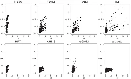
For each possible combination of parameter values (i.e., de-sign), I generate 5000 samples. Then I compute the median bias, the 75th–25th interquartile range (iqr), and the median absolute error (MAE) for all of the estimators evaluated, that is, GMM, SNM, LIML, AHNS, ssLIML, sGMM, HPT, and LSDV (means and standard deviations are not reported because SNM, LIML, and ssLIML estimators are expected to have infinite moments). The large number of designs considered precludes the dis-cussion of all of the results in detail. Based on MAEs,Figure 1 depicts an overview of the relative performance of the estimators for all of the DGPs considered with (N, T)=(50,4).Figure 1 presents MAEs forα(y-axis) andβ(x-axis) when the DGPs are mean-stationary.
MAEs corresponding to the LSDV estimator present the ex-pected pattern (large MAEs forα, while MAEs forβare rela-tively large only whenσξ2is small regardless of the feedback; moreover, LSDV presents the lowest iqrs). In the case of GMM, MAEs are of similar magnitude forαandβand relatively large in both cases, especially for large values ofσ2
η andα. SNM
presents systematically lower biases for bothαandβ but also
0
Figure 1. Median absolute errors (MAEs) under mean-stationarity. This figure presents the MAEs for all estimators ofαandβcorresponding to all the designs considered in our simulations under mean-stationarity.
larger iqrs, and thus MAEs are relatively similar to those of GMM. The AHNS estimator presents both lower biases and iqrs resulting in a better performance in terms of MAEs, especially in the case ofα. In contrast, LIML suffers from large biases and iqrs whenσξ2is large relative toση2so that its overall performance is relatively worse than the other estimators. The sGMM estimator performs relatively well under mean-stationarity and, overall, it seems to be preferable to GMM, SNM, and LIML (note that in many designs, there are no individual effects and then sGMM is expected to perform well). ssLIML presents MAEs similar to AHNS (slightly lower forαand larger forβ) caused by lower biases for bothαandβtogether with larger iqrs forβ. Also, the performance of the HPT estimator is similar to that of AHNS and ssLIML (a bit better forβ and somewhat worse for α), given its lower iqrs and slightly larger biases. Overall, MAEs inFigure 1seem to favor AHNS, HPT, and ssLIML over other estimators.
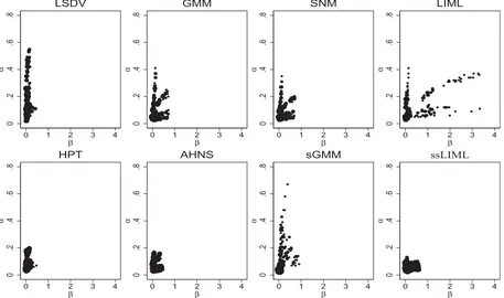
Figure 2 plots MAEs in the case of mean-nonstationarity designs. Overall, one can conclude that the relative perfor-mance of the competing estimators is very similar to that of mean-stationary settings. This is so because, with the excep-tion of sGMM, the considered estimators do not require mean-stationarity for fixed-T consistency. Therefore, only sGMM tends to present larger MAEs, thus performing considerably worse than in the case of mean-stationary DGPs. Moreover, for large values ofσ2
η relative toσv2, they all improve because
the correlation between lagged levels and first differences gets larger as shown in Hayakawa (2009). Note also that many MAEs plotted in Figures1and2correspond to designs withσ2
η =0, so
the effect of mean-stationarity assumptions becomes negligible. Finally, it is worth stressing that very different configurations
are “aggregated” in Figures 1 and2, so the resulting picture should be interpreted with caution.
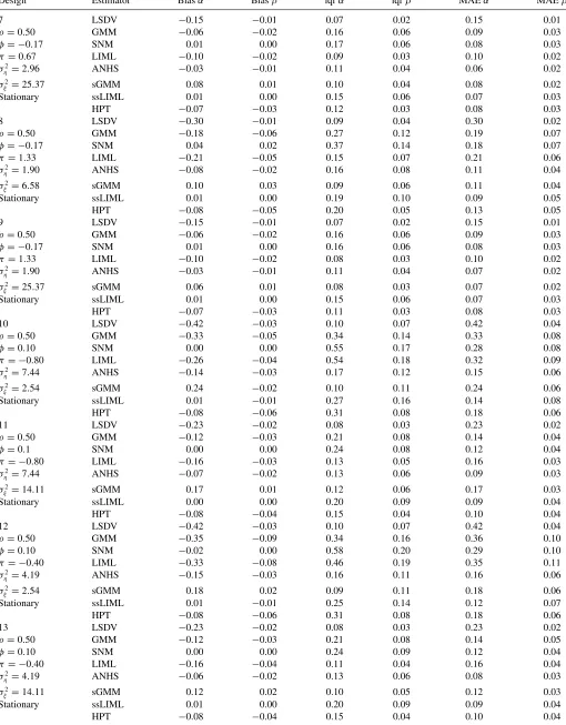
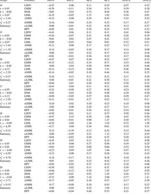
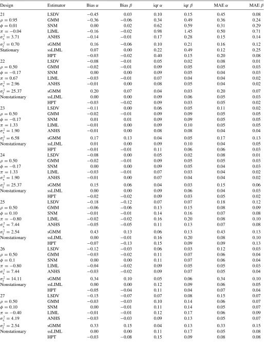
InTable 1, I analyze in detail simulation results for six differ-ent designs with (N, T)=(50,4).20In Design 1, there are no individual effects and the regressor is strictly exogenous. Un-der these circumstances, all of the estimators perform relatively well, biases are negligible, and iqrs are similar across estimators (only the LSDV estimator suffers from nonnegligible bias inα). Design 2 includes individual effects correlated with the strictly exogenous regressor under mean-stationarity. While the performance of LSDV is not affected by the individual effects, the biases in GMM, SNM, LIML, and AHNS double with re-spect to Design 1 with no individual effects (the increase in the biases for sGMM is even larger). This finding is in accordance with the analytical biases derived in Bun and Kiviet (2006) for method-of-moments estimators of this type. Finally, the bi-ases for the likelihood-based estimators considered (ssLIML and HPT) remain unaffected in absolute value when including individual effects in the DGP.
Design 3 explores the effects of varyingα, that is, the persis-tence of theyprocess. In this setting, increasingαalso increases the variance ofxitin Design 3 with respect to Design 1. Despite
a higherσ2
ξ contributes to improve the performance of the
es-timators, the increase in the persistence ofyshould deteriorate the quality of αestimates.21 Indeed, biases and iqrs forα are
20PopulationR2of the designs range from 0.76 to 0.90. On the other hand, all
designs inTable 1are based onρ=0.5.Table A1in the AppendixA.3includes additional results for designs withρ=0.95.
21Note that, according to the GMM perspective, instruments become weaker as
αorσ2
ηincreases under mean-stationarity.
0
Figure 2. MAEs under mean-nonstationarity. This figure presents the median absolute errors (MAEs) for all estimators ofαandβ corre-sponding to all the designs considered in our simulations under mean-nonstationarity.
now substantially larger in absolute value (with the exception of SNM, whose bias remains unaffected). With respect toβ, the biases are only slightly larger to those of Design 1, while the iqrs are very similar.
Design 4 explores the case of predetermined x(instead of strictly exogenous) with no individual effects. The overall per-formance of the estimators in terms of biases and iqrs is slightly better than that of Design 3. The largerσ2
ξ in Design 4
appar-ently offsets the effect of consideringφ=0. Hence, the effect of having predeterminedxinstead of strictly exogenousxseems to be moderate when α is substantial. This finding is also in accordance with the results in Bun and Kiviet (2006).
In contrast to Design 4, Design 5 includes individual effects in the model. Therefore, Design 5 considers feedback from laggedyto currentxtogether with individual effects correlated with the regressors, which is the main focus of this article. We see that biases are larger in comparison to Design 4; only ssLIML presents smaller biases as we increaseση2. Overall, only SNM and ssLIML present negligible biases in Design 5. Turning to dispersion, SNM has larger iqrs than ssLIML, and AHNS presents relatively small iqrs so that AHNS and ssLIML seem to be the preferred estimators in terms of MAEs under Design 5. This result is confirmed in all of the other designs with|φ| =0,
|π| =0,α=0.75, andσ2
η >1, which are reported in Appendix
A.3(seeTable A1).22
Design 6 considers Design 5 under mean-nonstationarity. Not surprisingly, sGMM suffers from larger and substantial
22Detailed results for all of the designs considered and plotted in Figures1and
2are available upon request.
biases under mean-nonnonstationarity. In contrast, all of the remaining estimators present smaller biases than in Design 5 (in the GMM setting, Hayakawa (2009) showed that, under mean-nonstationarity, “the instruments become stronger” whenση2is larger thanσv2). SNM and ssLIML deserve a special mention, as they now have zero bias for bothαandβ. Also, iqrs are now smaller than in Design 5 and similar across estimators. In terms of MAEs, GMM, SNM, LIML, and ssLIML perform surpris-ingly similar while AHNS presents the lowest MAEs for bothα
andβ.
InTable 2, I rerun Design 5 upon varying the sample sizes (N, T) and the distribution of the disturbances. First, when in-creasing N, the biases and iqrs of the GMM, SNM, AHNS, sGMM, HPT, and ssLIML estimators decrease as expected, given their fixed-T and large-N consistency. Nevertheless, the biases of LSDV and LIML are barely affected (see variant A in Table 2). I then explore the effects of increasingTforN =50 in variant B; interestingly enough, increasingTreduces the biases and iqrs for all of the estimators considered (only SNM seems to suffer from slightly larger biases inαasTincreases).
Variants C and D inTable 2explore fat-tailed and skew dis-turbances forN =50,T =4. On the one hand, I assume that all errors in the DGP are distributed as a Student’st-test with 4 degrees of freedom, implying an infinite kurtosis; that is, fat-ter tails than the normal distribution. On the other hand, I also explore errors distributed according to a mixture of two normal distributions with different means (being the difference equal to 50) so that the resulting distribution is nonsymmetric. For both nonnormal disturbances, the results are virtually unaltered with respect to the normal case. Moreover, for other fat-tailed and
Table 1. Simulation results forN =50,T =4
Design Estimator Biasα Biasβ iqrα iqrβ MAEα MAEβ
1 LSDV −0.13 0.00 0.07 0.07 0.13 0.03
α=0.25 GMM −0.02 −0.01 0.09 0.11 0.05 0.05
φ=0.00 SNM −0.01 0.00 0.09 0.11 0.05 0.05
π=0.00 LIML −0.02 0.00 0.09 0.11 0.05 0.06 σ2
η=0.00 ANHS −0.01 −0.01 0.09 0.11 0.05 0.05
σ2
ξ =2.85 sGMM −0.01 0.00 0.08 0.09 0.04 0.04
Stationary ssLIML −0.01 −0.01 0.08 0.14 0.04 0.07 HPT −0.02 −0.02 0.10 0.08 0.05 0.05
2 LSDV −0.13 0.00 0.07 0.07 0.13 0.04
α=0.25 GMM −0.04 −0.02 0.12 0.15 0.07 0.08 φ=0.00 SNM −0.02 −0.01 0.14 0.15 0.07 0.08 π=0.50 LIML −0.04 −0.02 0.13 0.15 0.07 0.08 σ2
η=4.90 ANHS −0.02 −0.01 0.10 0.12 0.05 0.06
σ2
ξ =2.85 sGMM 0.12 0.09 0.12 0.13 0.12 0.10
Stationary ssLIML 0.01 0.01 0.12 0.16 0.06 0.08 HPT −0.02 −0.03 0.11 0.08 0.06 0.05
3 LSDV −0.37 −0.02 0.10 0.06 0.37 0.03
α=0.75 GMM −0.10 −0.03 0.18 0.10 0.12 0.06
φ=0.00 SNM −0.01 0.00 0.20 0.11 0.10 0.05
π=0.00 LIML −0.07 −0.02 0.20 0.11 0.11 0.06 σ2
η=0.00 ANHS −0.09 −0.02 0.15 0.10 0.10 0.05
σ2
ξ =4.09 sGMM −0.04 0.00 0.13 0.08 0.07 0.04
Stationary ssLIML −0.04 −0.02 0.12 0.12 0.07 0.06 HPT −0.08 −0.05 0.24 0.07 0.15 0.06
4 LSDV −0.30 −0.01 0.10 0.04 0.30 0.02
α=0.75 GMM −0.06 −0.02 0.15 0.08 0.09 0.04
φ= −0.17 SNM 0.01 0.00 0.17 0.08 0.08 0.04
π=0.00 LIML −0.06 −0.02 0.16 0.08 0.09 0.04 σ2
η=0.00 ANHS −0.06 −0.02 0.14 0.08 0.08 0.04
σ2
ξ =6.58 sGMM −0.03 −0.01 0.12 0.06 0.06 0.03
Stationary ssLIML −0.04 −0.02 0.12 0.09 0.06 0.05 HPT −0.08 −0.05 0.20 0.05 0.13 0.05
5 LSDV −0.31 −0.01 0.10 0.04 0.31 0.02
α=0.75 GMM −0.20 −0.06 0.27 0.11 0.21 0.07
φ= −0.17 SNM 0.02 0.01 0.35 0.13 0.17 0.06
π=0.67 LIML −0.22 −0.05 0.16 0.07 0.22 0.06 σ2
η=2.96 ANHS −0.09 −0.02 0.15 0.07 0.11 0.04
σ2
ξ =6.58 sGMM 0.14 0.03 0.10 0.06 0.14 0.04
Stationary ssLIML 0.01 0.00 0.21 0.10 0.11 0.05 HPT −0.07 −0.05 0.20 0.05 0.12 0.05
6 LSDV −0.11 −0.01 0.06 0.05 0.11 0.02
α=0.75 GMM −0.02 −0.01 0.10 0.09 0.05 0.05
φ= −0.17 SNM 0.00 0.00 0.10 0.09 0.05 0.05
π=0.67 LIML −0.02 −0.01 0.10 0.10 0.05 0.05 σ2
η=2.96 ANHS −0.02 −0.01 0.08 0.08 0.04 0.04
σ2
ξ =6.58 sGMM 0.24 0.14 0.04 0.06 0.24 0.14
Nonstationary ssLIML 0.00 0.00 0.10 0.10 0.05 0.05 HPT −0.02 −0.03 0.11 0.06 0.06 0.03
NOTE: 5000 replications; bias refers to the estimation errors ˆα−αand ˆβ−β; iqr is the 75th–25th interquartile range; MAE denotes the median absolute error. In all designs, we fix
ρ=0.5.
skew disturbances, I find similar results, so to save space, they are not reported here.
Finally, the effects of considering (time-series) heteroscedas-tic disturbances are also investigated in Table 2. In par-ticular, Design 5 in Table 1 imposes σ2
v,t =σ
2
v =1.00 ∀t
and σξ,t2 =σξ2=6.58 ∀t; in contrast, for T =4, I consider
{σ2
v,0, σv,21, σv,22, σv,23, σv,24} = {1.00,0.50,0.75,1.25,1.50} and
{σ2
ξ,0, σ 2
ξ,1, σ 2
ξ,2, σ 2
ξ,3, σ 2
ξ,4} = {6.58,4.58,5.58,7.58,8.58} so that the time-series averages of the variances coincide with the time-series homoscedastic variances in Design 5, that is,
¯
σ2
v =1.00 and ¯σξ2=6.58.
Turning to the results in variant E, we first recall that, with the exception of HPT, all of the estimators evaluated here do not require time-series homoscedasticity for consistency; hence, we
Table 2. Simulation results for variants of Design 5
A: LSDV −0.35 −0.02 0.03 0.01 0.35 0.02
Sample: GMM −0.04 −0.01 0.13 0.05 0.07 0.03 N=500, T =4 SNM 0.00 0.00 0.13 0.05 0.07 0.03 Disturbances: LIML −0.22 −0.06 0.04 0.02 0.22 0.06 Standard Normal ANHS −0.02 −0.01 0.10 0.04 0.05 0.02 Homoscedastic sGMM 0.02 0.00 0.06 0.02 0.03 0.01 ssLIML 0.00 0.00 0.09 0.04 0.05 0.02 HPT −0.06 −0.05 0.06 0.02 0.07 0.04
B: LSDV −0.06 0.01 0.03 0.02 0.06 0.01
Sample: GMM −0.05 0.00 0.04 0.02 0.05 0.01 N=50, T =16 SNM 0.06 0.01 0.04 0.02 0.06 0.01 Disturbances: LIML −0.03 0.00 0.07 0.02 0.04 0.01 Standard Normal ANHS −0.05 0.00 0.04 0.02 0.05 0.01 Homoscedastic sGMM 0.07 0.01 0.05 0.02 0.07 0.01 ssLIML 0.00 0.00 0.05 0.03 0.02 0.01 HPT −0.03 −0.02 0.04 0.02 0.03 0.02
C: LSDV −0.35 −0.02 0.12 0.05 0.35 0.03
Sample: GMM −0.19 −0.06 0.27 0.11 0.21 0.07 N=50, T =4 SNM 0.04 0.02 0.41 0.15 0.19 0.07 Disturbances: LIML −0.24 −0.06 0.16 0.07 0.24 0.06 Student 4 df ANHS −0.09 −0.02 0.17 0.08 0.12 0.05 Homoscedastic sGMM 0.12 0.02 0.10 0.06 0.12 0.03 ssLIML −0.02 −0.01 0.17 0.10 0.08 0.05 HPT −0.08 −0.05 0.22 0.05 0.13 0.05
D: LSDV −0.35 −0.02 0.10 0.04 0.35 0.03
Sample: GMM −0.20 −0.06 0.27 0.12 0.21 0.07 N=50, T =4 SNM 0.03 0.02 0.38 0.14 0.18 0.07 Disturbances: LIML −0.24 −0.06 0.16 0.07 0.24 0.06 Mixture of Normals ANHS −0.10 −0.03 0.17 0.08 0.13 0.05 Homoscedastic sGMM 0.12 0.02 0.10 0.06 0.12 0.03 ssLIML −0.02 −0.01 0.19 0.10 0.10 0.05 HPT −0.08 −0.06 0.21 0.06 0.12 0.06
E: LSDV −0.41 −0.04 0.09 0.04 0.41 0.04
Sample: GMM −0.19 −0.06 0.23 0.10 0.19 0.07 N=50, T =4 SNM −0.02 0.00 0.30 0.12 0.15 0.06 Disturbances: LIML −0.26 −0.07 0.15 0.07 0.26 0.07 Standard Normal ANHS −0.12 −0.03 0.16 0.08 0.13 0.05 TS Heteroscedastic sGMM 0.11 0.02 0.09 0.06 0.11 0.04 ssLIML −0.02 −0.01 0.18 0.09 0.08 0.05 HPT −0.22 −0.06 0.16 0.05 0.23 0.06
NOTES: 5000 replications; bias refers to the estimation errors ˆα−αand ˆβ−β; iqr is the 75th–25th interquartile range; MAE denotes the median absolute error. Parameter values common to all variants correspond to Design 5, that is,α=0.75,φ= −0.17,π=0.67, andσ2
η=2.96. Variants A and B consider sample sizes different from the baselineN=50, T=4
in Table 1; variants C and D explore nonnormal disturbances; variant E investigates the effects of time-series (TS) heteroscedasticity on the finite sample performance of the estima-tors, that is,{σ2
v,0, σv,21, σv,22, σv,23, σv,24} = {1.00,0.50,0.75,1.25,1.50}and{σξ,20, σξ,21, σξ,22, σξ,23, σξ,24} = {6.58,4.58,5.58,7.58,8.58}instead ofσv,t2 =σv2=1.00∀tandσξ,t2 =σξ2=
6.58∀t.
expect their performance to remain unaltered under time-series heteroscedasticity. Indeed, the estimates reported in variant E show some differences with respect to those of Design 5 in Table 1, albeit small. In contrast, the performance of the HPT estimator deteriorates (especially forα) under time-series het-eroscedasticity.
Tests of hypothesis and confidence intervals are usually based on “tstatistics” asymptotically distributed as a standard normal distribution.23Therefore, it is worth exploring the corresponding
finite-sample distributions of theset statistics and comparing them with the N(0,1) distribution. For this purpose,Table 3
23Thesetstatistics are calculated ast
=( ˆα−α)/ˆσ( ˆα) andt=( ˆβ−β)/ˆσ( ˆβ), where ˆσ( ˆα) and ˆσ( ˆβ) refer to the estimated asymptotic standard errors of the estimators ˆαand ˆβ.
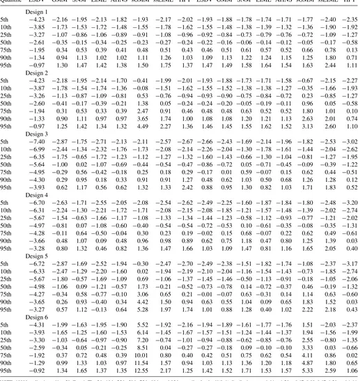
reports the finite-sample quantiles of thetstatistics. In particular, I explore the six designs inTable 1based on 10,000 replications, given the interest here in the upper tail of the distribution.
Looking at the median, the distributions of the LSDV, GMM, LIML, AHNS, and HPTtstatistics are generally shifted to the left for bothα andβ. Moreover, while the absolute value of the shift tends to increase with ση2, it decreases with σξ2. In contrast, the distributions of SNM and ssLIMLt statistics are overall more centered, especially in Designs 5 and 6 where both the individual effects and the predetermined explanatory variable are present. Under these two designs, theN(0,1) ap-proximation is particularly inaccurate for the case of sGMMt
statistics.
Turning to the upper quantiles, ssLIMLt statistics present thicker tails for both parameters. In the case ofα, the differences
Table 3. Quantiles of thetstatistics
α β
Quantile LSDV GMM SNM LIML AHNS sGMM ssLIML HPT LSDV GMM SNM LIML AHNS sGMM ssLIML HPT
Design 1
5th −4.23 −2.16 −1.95 −2.13 −1.82 −1.93 −2.17 −2.02 −1.93 −1.88 −1.78 −1.74 −1.71 −1.77 −2.40 −2.35 10th −3.85 −1.73 −1.53 −1.72 −1.48 −1.55 −1.78 −1.62 −1.55 −1.48 −1.38 −1.39 −1.32 −1.36 −1.90 −1.92 25th −3.27 −1.07 −0.86 −1.06 −0.89 −0.91 −1.08 −0.96 −0.92 −0.84 −0.73 −0.79 −0.76 −0.72 −1.09 −1.27 50th −2.61 −0.35 −0.15 −0.34 −0.25 −0.23 −0.27 −0.24 −0.22 −0.16 −0.06 −0.14 −0.12 −0.05 −0.17 −0.58 75th −1.95 0.34 0.53 0.39 0.41 0.48 0.51 0.43 0.46 0.51 0.61 0.57 0.52 0.66 0.78 0.13 90th −1.34 0.94 1.13 1.02 1.02 1.11 1.26 1.03 1.09 1.13 1.22 1.24 1.15 1.25 1.80 0.71 95th −0.97 1.30 1.47 1.42 1.38 1.50 1.75 1.37 1.47 1.49 1.58 1.64 1.54 1.63 2.44 1.11
Design 2
5th −4.23 −2.18 −1.95 −2.14 −1.70 −0.41 −1.99 −2.01 −1.93 −1.88 −1.73 −1.71 −1.58 −0.67 −2.15 −2.27 10th −3.87 −1.78 −1.54 −1.74 −1.36 −0.08 −1.51 −1.62 −1.55 −1.52 −1.38 −1.38 −1.27 −0.35 −1.66 −1.93 25th −3.26 −1.13 −0.87 −1.09 −0.81 0.53 −0.76 −0.94 −0.93 −0.90 −0.75 −0.84 −0.72 0.23 −0.85 −1.27 50th −2.60 −0.41 −0.17 −0.39 −0.21 1.38 0.05 −0.24 −0.24 −0.20 −0.05 −0.19 −0.11 0.96 0.05 −0.58 75th −1.94 0.31 0.53 0.33 0.39 2.47 0.91 0.46 0.48 0.48 0.63 0.52 0.52 1.80 1.01 0.10 90th −1.33 0.90 1.11 0.97 0.97 3.65 1.74 1.00 1.08 1.08 1.20 1.21 1.13 2.63 2.01 0.74 95th −0.97 1.25 1.42 1.34 1.32 4.49 2.27 1.36 1.46 1.45 1.55 1.62 1.52 3.13 2.60 1.10
Design 3
5th −7.40 −2.87 −1.75 −2.71 −2.13 −2.11 −2.57 −2.67 −2.66 −2.43 −1.69 −2.14 −1.96 −1.82 −2.53 −3.02 10th −6.99 −2.44 −1.34 −2.32 −1.76 −1.73 −2.08 −2.14 −2.26 −2.04 −1.30 −1.78 −1.61 −1.44 −2.04 −2.62 25th −6.35 −1.75 −0.65 −1.72 −1.23 −1.12 −1.27 −1.32 −1.60 −1.43 −0.66 −1.30 −1.04 −0.81 −1.27 −1.95 50th −5.64 −1.00 0.02 −1.07 −0.69 −0.44 −0.54 −0.47 −0.86 −0.72 0.05 −0.71 −0.45 −0.09 −0.39 −1.22 75th −4.95 −0.29 0.56 −0.42 −0.18 0.25 0.18 0.29 −0.17 0.01 0.59 −0.07 0.15 0.62 0.44 −0.51 90th −4.30 0.29 0.95 0.18 0.33 0.91 0.91 1.27 0.48 0.62 1.03 0.50 0.68 1.26 1.28 0.12 95th −3.93 0.62 1.17 0.56 0.62 1.32 1.33 2.42 0.88 0.95 1.30 0.82 1.03 1.71 1.83 0.52
Design 4
5th −6.70 −2.63 −1.71 −2.55 −2.05 −2.08 −2.54 −2.62 −2.49 −2.25 −1.60 −1.87 −1.84 −1.80 −2.48 −3.20 10th −6.31 −2.24 −1.30 −2.21 −1.72 −1.71 −2.08 −2.15 −2.08 −1.85 −1.21 −1.57 −1.48 −1.39 −2.02 −2.74 25th −5.67 −1.54 −0.63 −1.66 −1.17 −1.08 −1.33 −1.34 −1.44 −1.23 −0.58 −1.12 −0.93 −0.77 −1.21 −2.02 50th −4.97 −0.81 0.07 −1.08 −0.60 −0.40 −0.54 −0.54 −0.72 −0.53 0.10 −0.61 −0.35 −0.08 −0.35 −1.31 75th −4.28 −0.11 0.64 −0.50 −0.04 0.30 0.23 0.19 −0.02 0.15 0.68 −0.07 0.22 0.62 0.49 −0.61 90th −3.66 0.48 1.07 0.09 0.48 0.96 0.98 0.89 0.62 0.75 1.18 0.47 0.80 1.25 1.39 0.03 95th −3.28 0.80 1.32 0.46 0.82 1.36 1.47 1.66 1.03 1.09 1.47 0.81 1.16 1.65 2.05 0.40
Design 5
5th −6.72 −2.87 −1.69 −2.52 −1.94 −0.30 −2.47 −2.70 −2.49 −2.38 −1.51 −1.82 −1.74 −1.08 −2.37 −3.17 10th −6.33 −2.47 −1.29 −2.20 −1.60 0.02 −1.94 −2.19 −2.10 −2.04 −1.16 −1.54 −1.43 −0.73 −1.85 −2.74 25th −5.67 −1.80 −0.57 −1.69 −1.09 0.69 −1.06 −1.37 −1.45 −1.46 −0.50 −1.13 −0.91 −0.18 −1.05 −2.06 50th −4.98 −1.06 0.09 −1.21 −0.57 1.73 −0.21 −0.52 −0.73 −0.78 0.14 −0.72 −0.37 0.46 −0.19 −1.32 75th −4.27 −0.34 0.58 −0.77 −0.10 3.06 0.65 0.21 −0.01 −0.07 0.63 −0.31 0.14 1.14 0.63 −0.60 90th −3.65 0.26 0.93 −0.40 0.34 4.42 1.50 0.94 0.63 0.55 1.04 0.09 0.65 1.83 1.52 0.03 95th −3.27 0.57 1.12 −0.13 0.64 5.28 1.97 1.74 1.01 0.88 1.28 0.40 1.02 2.22 2.18 0.43
Design 6
5th −4.31 −1.99 −1.63 −1.95 −1.90 5.52 −1.92 −2.16 −1.94 −1.89 −1.61 −1.77 −1.76 1.51 −2.03 −2.37 10th −3.93 −1.65 −1.25 −1.60 −1.53 6.14 −1.45 −1.67 −1.57 −1.51 −1.24 −1.44 −1.37 1.94 −1.56 −1.99 25th −3.30 −1.03 −0.64 −0.97 −0.90 7.20 −0.74 −1.01 −0.94 −0.88 −0.62 −0.85 −0.76 2.55 −0.80 −1.35 50th −2.59 −0.34 0.05 −0.21 −0.25 8.51 0.04 −0.27 −0.27 −0.18 0.09 −0.10 −0.10 3.33 0.03 −0.66 75th −1.92 0.37 0.72 0.48 0.39 10.01 0.80 0.40 0.42 0.51 0.75 0.62 0.54 4.11 0.86 0.02 90th −1.29 0.99 1.33 1.03 0.97 11.54 1.57 0.94 1.03 1.13 1.36 1.20 1.18 4.87 1.80 0.65 95th −0.92 1.34 1.65 1.37 1.35 12.55 2.17 1.25 1.42 1.52 1.71 1.53 1.57 5.33 2.59 1.06
NOTE: 10000 replications;N=50, T=4; The 5th, 10th, 25th, 50th, 75th, 90th, and 95th quantiles for theN(0,1) distribution are−1.64,−1.28,−0.67,0.00,0.67,1.28, and 1.64, respectively.
with the correspondingN(0,1) quantiles are generally smaller for ssLIML and SNM than for the other estimators considered; however, these differences are generally larger for ssLIML in the case ofβ. All in all, the normal approximation works reasonably well for ssLIML in the case of theαparameter; in contrast, for theβcoefficient, ssLIML exhibits thick tails.
4. EMPIRICAL APPLICATION: INCOME AND DEMOCRACY
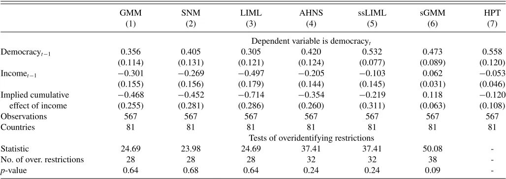
In an influential article, Acemoglu et al. (2008) estimated the effect of income on democracy in a panel of countries that spans the last part of the 20th century. In particular, they consider the