Full Terms & Conditions of access and use can be found at
http://www.tandfonline.com/action/journalInformation?journalCode=ubes20
Download by: [Universitas Maritim Raja Ali Haji] Date: 12 January 2016, At: 22:50
Journal of Business & Economic Statistics
ISSN: 0735-0015 (Print) 1537-2707 (Online) Journal homepage: http://www.tandfonline.com/loi/ubes20
Dynamic Treatment Assignment
Peter Fredriksson & Per Johansson
To cite this article: Peter Fredriksson & Per Johansson (2008) Dynamic Treatment Assignment, Journal of Business & Economic Statistics, 26:4, 435-445, DOI: 10.1198/073500108000000033
To link to this article: http://dx.doi.org/10.1198/073500108000000033
Published online: 01 Jan 2012.
Submit your article to this journal
Article views: 268
View related articles
Dynamic Treatment Assignment:
The Consequences for Evaluations
Using Observational Data
Peter F
REDRIKSSONInstitute for Labour Market Policy Evaluation (IFAU) and Department of Economics, Uppsala University, Uppsala,
Sweden (peter.fredriksson@ifau.uu.se)
Per J
OHANSSONInstitute for Labour Market Policy Evaluation (IFAU) and Department of Economics, Uppsala University, Uppsala,
Sweden (per.johansson@ifau.uu.se)
We discuss estimation of treatment effects when the timing of treatment is the outcome of a stochastic process. We show that the duration framework in discrete time provides a fertile ground for effect evalu-ations. We suggest easy-to-use nonparametric survival function matching estimators that can be used to estimate the time profile of the treatment. We study the small-sample properties of the proposed estimators and apply one of them to evaluate the effects of an employment subsidy program. We find that the longer-run program effects are positive. The estimated time profile suggests locking-in effects while participating in the program and a significant upward jump in the employment hazard on program completion. KEY WORDS: Dynamic treatment assignment; Method of matching; Program evaluation; Treatment
effects.
1. INTRODUCTION
The prototypical evaluation problem is cast in a framework in which treatment is offered only once. Thus treatment assign-ment is a static problem, and the information contained in the timing of treatment is typically ignored (see Heckman, Lalonde, and Smith 1999 and Imbens 2004 for overviews of the litera-ture). This prototype concurs rather poorly with how most real-world programs work. Often it makes more sense to think of the assignment to treatment as a dynamic process, where the start of treatment is the outcome of a stochastic process.
This article is concerned with program evaluations when (a) there are no restrictions on the timing of the individual treat-ment and (b) the timing of treattreat-ment is linked to the potential outcome of interest. Evaluations of labor market programs of-ten include these two features. A common evaluation problem is when individuals may enter, for instance, a training program at any time during the unemployment spell and interest lies in the employment effects of this training program. This situation can raise complex simultaneity issues, because both the out-come of interest (employment) and actual treatment status are functions of potential unemployment duration; even if intended treatment status were randomized at the time of unemployment entry, dynamic selection would determine actual treatment sta-tus if a time span existed between randomization and the start of treatment.
Our main objective is thus to discuss estimation of treatment effects when assignment to treatment is without restrictions on when to participate (i.e., it is the outcome of an stochastic process). We propose an estimator of the effect of treatment on the treated in this situation and examine the small-sample prop-erties of this estimator using Monte Carlo simulations. Finally, we illustrate the evaluation problem and the usefulness of the estimator in an empirical application.
The empirical evaluation concerns the effect of an em-ployment subsidy (ES) program on future emem-ployment. These
data were previously analyzed by Forslund, Johansson, and Lindquist (2004). The subsidy was targeted at the long-term un-employed, registered as unemployed at the public employment service (PES) for at least 12 months. The subsidy amounted to 50% of total wage costs and was paid for a maximum of 6 months. This evaluation problem has the features de-scribed above because after having become eligible (i.e., after 12 months), the subsidy program may start at any point in time. In general, two types of approaches have been used in pre-vious work to analyze the evaluation problem that we consider here. One of these is to try to estimate the effect of treatment on the treated on the employment propensity some fixed time period after treatment; a recent example of this was provided by Gerfin and Lechner (2002). In this approach, it is common to use nonparametric matching procedures and to regard treat-ment assigntreat-ment as a static problem. The other common ap-proach is to estimate the effect on the hazard to employment. Usually, more structure is imposed on the form of the hazard, but there is also greater concern about unobserved heterogene-ity than in the first approach. The most recent work (e.g., Ab-bring and van den Berg 2003; van den Berg, van der Klaauw, and van Ours 2004) in this vein has explicitly recognized that treatment assignment is a dynamic process and has shown that if sufficient structure is imposed, this can be useful for identifi-cation purposes. Abbring and van den Berg (2003) showed that a (homogenous) treatment effect can be identified, assuming a mixed proportional hazards model in discrete time.
The estimator that we propose here uses elements from both of these approaches. It is a nonparametric matching estimator in discrete time. But unlike most estimators that take a matching approach, the estimator recognizes that treatment assignment
© 2008 American Statistical Association Journal of Business & Economic Statistics October 2008, Vol. 26, No. 4 DOI 10.1198/073500108000000033 435
is a dynamic process; assuming that the process of treatment assignment is static inevitably yields a biased estimator.
Compared with the approach of Abbring and van den Berg (2003), we thus can be more flexible in terms of specifying the hazard; the cost of this added flexibility is that we must assume that unobserved heterogeneity does not simultaneously deter-mine the duration to employment if not treated and the duration to treatment.
We focus on estimating the additive effect of entering ES on the survival probability in unemployment for those enter-ing this program. If the appropriate conditional independence assumptions are fulfilled, we can estimate the time profile of such treatment effects. Moreover, we can estimate treatment fects for different entry time points, as well as the overall ef-fect of the program averaged over pretreatment durations. This overall estimate is akin to the treatment effect estimated in a randomized experiment in which actual treatment status is ran-domized among the stock of eligibles. Our matching estimator of the overall effect balances the pretreatment durations in the treated and comparison groups in the same way as random as-signment in the experiment.
Estimating the time profile of treatment effects is particularly interesting when it comes to the evaluation of labor market pro-grams. Usually we think of program participation as an invest-ment in current time (and money) for a potential increase in the future employment probability. We would expect search activ-ity to be decreased during the in-program period—that is, there is a locking-in effect—whereas the outflow to employment may increase after program completion.
The results from the empirical application concur with this prior. During the first 6 months after entry into the subsidy program, the employment outflow is lower among the treated; this locking-in effect is particularly evident for those who enter early after becoming eligible. After the maximum duration of the program (i.e., after 6 months), a sharp increase in the em-ployment hazard occurs. One may interpret the peak occurring after program completion as evidence of displacement effects; employers use the subsidy to fill vacancies that otherwise would be filled by hiring on the regular market.
The rest of this article is organized as follows. In Section 2 we present the evaluation framework. In Section 3 we consider es-timation and inference, and suggest an estimator of the effect of treatment on the treated on the survival rate in unemployment, that is based on a discrete time assumption. In Section 4 we study the small-sample performance of this estimator. In Sec-tion 5 we estimate the effects of the employment subsidy pro-gram on the survival rate in unemployment for those entering the ES program. We present some conclusions in Section 6.
2. THE EVALUATION FRAMEWORK
We consider a pool of workers, indexed byi=1, . . . ,N, who became unemployed on the same date. These individuals are all eligible for the program as long as they stay unemployed. These individuals are exposed to two types of risk at time t: either they get a job offer, with probabilityλ0(t)per unit time, or they get an offer to participate in a treatment (a program), with probabilityγ (t)per unit time. We make the following key assumption concerning the job hazard and the program entry hazard at timet:
Assumption(unconfoundedness).
λ0i(t)=λ0(t), γi(t)=γ (t).
In other words, these two hazards are assumed to be identi-cal across individuals conditional on the date of unemployment entry and observed covariates. (Note that we surpress observed covariates for most of our analysis.)
This assumption implies competing risks; that is, there is no unobserved heterogeneity that jointly determines employment and treatment assignment. Note that, because our assumption rules out unobserved heterogeneity, it also rules out differences in the hazard att due to unobserved anticipation about future (t+1, . . .) events. (See Richardson and van den Berg 2001 for a good discussion of anticipation effects in a competing-risks framework.) Whether these assumptions are reasonable or not depends on the richness of the data and the application in ques-tion.
It is also important to note what is not implied by our key assumption. We emphasize two things: (a) There is no implied restriction on the variation in potential duration across individ-uals, and (b) the response to treatment may well vary across individuals (but they are not allowed to act on this heterogene-ity).
Let us introduce some notation to further illustrate the evalu-ation framework. LetT0denote potential unemployment dura-tion if not treated andSdenote the potential duration until treat-ment start. In this setting,Sis stochastically dependent onT0. Whether or not we observeSdepends, inter alia, on whether the individual had the luck to receive a job offer before receiving an offer to participate in treatment. In particular, the treatment indicator (D=1) is observed if and only if unemployment du-ration if not treated is longer than the time period until the start of the program,
D=1(T0>S), (1)
where1(·)is the indicator function. Note that the dynamic
treat-ment assigntreat-ment (1) is not an issue in the literature on sequen-tial treatments (e.g., Robins 1986; Lechner 2004). In this litera-ture, treatment is assumed to occur at the start of a given period, and the outcomes occur at the end of this period.
We introduce two additional potential outcomes. For individ-uals who have survived up tos, we defineW1(s)as survival time aftersif treated atsand;W0(s)as survival time aftersif not treated atsor thereafter. Furthermore, we define the treatment indicator
D(s)=1(T0>s). (2)
In general, there are (at least) two policy questions of interest. First, one may be interested in the effect of the program for those entering the program at a given duration. This parameter is defined as
1(s)=EW1(s)−W0(s)|D(s)=1. (3) This is a relevant parameter if one is interested mainly in the effectiveness of offering a treatment at different durations.
However, ideally one also would like to know the overall ef-fect of the program, that is, if the treatment reduces the average
duration in unemployment for all of those who enter the pro-gram. Thus the parameter of interest is
1=E(W1−W0|D=1), (4)
where E(W0|D=1)is the posttreatment duration for the treated if not treated. We now focus on the estimation of (4). The prob-lems encountered when estimating (4) also pertain when esti-mating (3).
Provided that there is no right-censoring of unemployment durations, it is possible to estimate E(W1|D=1)as
wheren1is the number of individuals receiving treatment. The evaluation problem involves not observing the posttreatment duration without treatment for the treated. What makes the eval-uation nonstandard in the dynamic treatment assignment setting is that we lack (treatment) start dates for those not treated. Thus only the pretreatment duration for the treated is observed. This is different than in the experimental situation, in which treat-ment for the stock of eligibles is offered at some fixed time point, and the fairly uncommon situation in which a program starts after a fixed time period.
One consequence of the data-generating process (1) is that the potential duration if not treated is longer for the treated than for the nontreated. Using the notation of Dawid (1979), this can be expressed as
W0⊥⊥D. (5)
Thus any attempt (e.g., Lechner 1999) to estimate treatment ef-fects based on the static treatment indicator,D, will yield biased estimates.
However, under the unconfoundedness assumption, the prob-ability distribution of the potential duration if not treated is in-dependent ofD(s), that is,
W0⊥⊥D(s). (6)
Equation (6) implies is that the estimator of E(W0|D=1)can be based on matching treated individuals atswith nontreated individuals at s. Applying this procedure, we get a matched-comparison sample and can estimate E(W0|D=1)as aftersifor a (randomly assigned) matched individual (ci).The treatment effect is then estimated as
c. If the treatment effects have the same sign for all entry durations, then1is biased toward 0.
Proof. The duration of the comparison individual, ci, is given as
Wci consists of two parts: the postduration as nontreated atsi and the difference in duration if treated and not treated from the time of treatment,Sci, if treated in the future (Sci >si). Thus the fact that comparison individuals may be treated in the future biases the estimate. If the treatment effects have the same sign for all entry durations, then the estimate is attenuated.
This estimator is useful only when it comes to testing for the existence of a treatment. In the realistic case where the treat-ment effects are of the same sign for all entry durations, the estimator is biased toward 0; thus this opportunity may be of little practical use.
To sum up this section, we have illustrated that any estimator of (4) using a time-invariant treatment indicator will be biased. This follows from the treatment assignment process (1), which implies (5). Transforming a world in which treatment assign-ment is the outcome of two stochastic processes to an idealized world in which treatment assignments and outcomes occur at single time points simply is not possible (see Fredriksson and Johansson 2004 for a detailed discussion). Because (6) holds, valid tests for treatment effects may be based on the observed duration and the time-varying treatment indicatorD(s). But the power of these tests is likely to be low, because the estimators are likely biased toward 0 if there is a treatment effect.
3. ESTIMATION AND INFERENCE IN
DISCRETE TIME
The previous section outlined a set of “impossibility results.” In this section we are more constructive and consider strate-gies to nonparametrically estimate and test for treatment effects when time is discrete. For all practical applications concerning unemployment durations, this assumption is not restrictive; it may be more restrictive in other circumstances, in which case one should bear in mind the potential bias caused by time aggre-gation. Also in this section we suppress observed heterogeneity. The extension to observed heterogeneity is relegated to the Ap-pendix because it is relatively straightforward.
3.1 Matching Estimator of the Survival Difference
Let us think of Wk(s), k=0,1, as being measured in dis-crete time. Then we define the potential employment out-comes in time period w if treated ats as follows:Y1(w,s)=
1(W1(s)=w) is the employment status at w if treated at s,
andY0(w,s)=1(W0(s)=w)is the employment status if not
treated atsor thereafter. Furthermore, we define the risk sets
Rk(w,s)=1(Wk(s)≥w), that is, the number of individuals
still at risk of employment atwshould they have treatment sta-tuskats.
The hazard rate for those treated atscan be estimated using the sample receiving treatment ats,
whereLdenotes calender time. (Here the censoring date is as-sumed to be independent of treatment status.)
How should the counterfactual hazard to employment be cal-culated? From (6), we have that for a given time period,s, treat-ment status contains no information about the potential post-treatment duration if not treated. The discrete-time equivalent to this condition is
{Y0(w,s)}∞w=1⊥⊥D(s), ∀s. (8)
Equation (8) follows from the unconfoundedness assump-tion. The implication of (8) is that censoring into a program is independent of the outcome. Thus we can compare the hazard rate for those who received treatment at swith those who did not. This implies that the estimates of the counterfactual hazard to employment for those treated atscan be based on those not yet treated ats,
Conditioning ons, the survival function for the treated and the counterfactual survival function can be estimated as
Fk(w,s)= w
u=1
(1−χk(u,s)), w=1, . . . ,L−s,k=0,1.
By the independence condition (8), we can calculate the effect of entering the program atsas the difference between the two survival functions, that is,
(w,s)=F1(w,s)−F0(w,s), w=1, . . . ,L−s. (9) Under the assumption of no treatment heterogeneity (across individuals), the variance of the estimator can be calculated as
is the asymptotic variance of the estimated survival functions based on the formula of Greenwood (1926) (see Kaplan and Meier 1958 for a justification).
This result implies that the variance can be consistently es-timated under the null hypothesis (i.e., no effect). Inference then can be based on the regularity conditions that yield as-ymptotic normality of the Kaplan–Meier estimator. If there is treatment heterogeneity, then asymptotic normal confidence in-tervals based on (10) most likely are too small (Imbens 2004).
A common approach to calculating the variance of matching es-timators is the bootstrap; however, Abadie and Imbens (2006) have shown that there is no theoretical justification for using the bootstrap to calculate the variance of matching estimators.
Aggregation Over Pretreatment Durations. The estimator defined by (9) has a clear interpretation; however, for policy analysis, one is generally interested in estimating the treatment effect for the entire treated population. If there are sufficient data such that (9) is estimable, then the most obvious way of aggregating over pretreatment durations is by taking the expec-tation over the distribution of treatment starts in the treated pop-ulation, that is, bility of having received treatment atsamong the treated who were still unemployed atw. Calculating the variance of this esti-mator is complicated by the fact that it is a function of two sto-chastic variables: the estimated treatment effects and the time until the start of treatment. The only conceivable option is to treat the distribution of the start of treatment as given. This im-plies that we are focusing on the “sample treatment effect,” that is, the average treatment effect for those treated in the data un-der consiun-deration (see Imbens 2004). Unun-der this assumption, the variance can be calculated as
var((w))=
The covariances arise because uncensored spells atsare poten-tially used to estimateFk(w,s′),k=0,1,ats′>s.
Estimating the variance defined in (12) is particularly dif-ficult. Moreover, estimating the conditional survival functions with precision may not be possible, because there are too few individuals at each (or some)s. This limits the uses of (11).
A more convenient way to average over the pretreatment du-ration is to first estimate the average hazard rate and then cal-culate the survival function. The average hazard rate for the treated is equal to
Given the independence condition (8), the average hazard rate for the treated if not treated can be estimated as
where p0(w,s) =R0(w,s)/Ls=0R0(w,s) is the estimated probability to be at risk atwif not treated atsfor the treated population.
Now the difference in these two averaged hazards has a clear interpretation. But if the main purpose of the analysis is to test for the existence of a treatment effect, then power—rather than interpretability—is the major issue. For the purpose of testing, consider the estimator
1(w)=F1(w)−F0(w), w=1, . . . ,L, (13)
whereFk(w)= wu=1(1−χk(u)), w=1, . . . ,L, k=0,1. In general, when the treatment effects vary with pretreatment du-ration, interpreting1(w)may be difficult, because it does not equal the difference in average survival rates due to treatment for the treated population. The estimator (13) does have two virtues, however. First, the power in rejecting a false null hy-pothesis is likely to be much greater than that when using an estimator based on the difference in the averaged hazards; sec-ond, if the hazard rates,χk(w,s), do not vary withs, then this estimator has a clean interpretation.
Note, finally, that the hazardχ0(w)and the survival function F0(w)define matching estimators. To apply these, we simply need to create the same distribution of pretreatment durations as for those who actually enter the program. The estimator (13) thus balances the pretreatment duration, analogously to what random assignment accomplishes in experimental data. Ran-dom assignment then balances the pretreatment duration (and any other covariates) for the treated and control groups, which is why we do not need to condition on the length of the period before treatment entry when estimating the treatment effect.
What about the variance of1(w)? The variance is equal to
var(1(w))=var(F0(w))+var(F1(w))
−2 cov(F1(w),F0(w)). (14)
Because individuals used as controls may be treated in the future and thus included in the estimation of both F0(w)
and F1(w′), w′ >w, there is a covariance term to worry about. We have that cov(F1(w),F0(w))=0 if w=1 and cov(F1(w),F0(w))=0, ∀w>1. With no treatment hetero-geneity (across individuals), we can apply the formula of Greenwood (1926) to estimate the two variances,
var(Fk(w))= [Fk(w)]2
×
w
u=1
ˆ
χk(u)
L
s=0[Rk(u,s)−
i∈D(s)=kYik(u,s)]
,
k=0,1.
The crux is to estimate the covariance term. At present, we have no solution. An (admittedly simple-minded) approach is to ig-nore the covariance. The approximation error involved is small if there are few treated individuals compared with the number of never treated individuals, because then the covariance is neg-ligible relative to the variance. In the next section, we present some Monte Carlo evidence to evaluate whether ignoring the covariance is a serious omission.
4. MONTE CARLO SIMULATION
Here we study the small-sample performance of the estima-tors introduced earlier. Toward this end, we assume thatT(0),
W(1), andSare geometrically distributed. Thus probability dis-tributions of the durations until employment and treatment are given by
Pr(Ti(0)=t)=p0(xi)q0(xi)t and
Pr(Si=s)=ps(xi)qs(xi)s.
Here p0(xi)=1−q0(xi)is the hazard rate if not treated and ps(xi)=(1−qs(xi))is the treatment hazard;p0(xi)andps(xi) are assumed to be logistic [i.e., p0(xi)=(1 +exp(−(a0+
a1xi)))−1,ps(xi)=(1+exp(−(b0+b1xi)))−1];x is taken to be uniformly distributed and fixed in repeated samples; and
a0= −3.0, b0= −6.5 or−5.5,andb1=a1is either 1 or 0. In the homogenous case (i.e., b1=a1=0), the exit hazard if not treated is.047 and the hazard into treatmentγ (t)is.0015 (b0= −6.5) or.0041 (b0= −5.5). The proportion treated is on average equal to 2.9% and 7.6% in these two situations encoun-tered. The case where 2.9% are treated resembles the situation encountered in the empirical application described in the next section. We also consider inference in a situation in which a larger fraction is treated.
The probability distribution of the duration until employment after having entered treatment atsis modeled as
Pr(Wi1(s)=w)=p1(xi)q1(xi)w,
wherep1(xi)=(1+exp(−(a0+as+a1xi)))−1is the exit haz-ard to employment. The no treatment effect situation is obtained withas =0, and the constant treatment effect situation is ob-tained withas=.69.In the case with no observed heterogene-ity, the difference in the hazard rate between treated and non-treated is 4.3%, that is,p1(xi)−p0(xi)=.043.
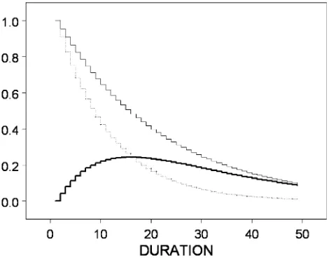
Figure 1 illustrates the two data-generating processes (treated and not treated) without heterogeneity and also shows the treat-ment effect (i.e., the difference between the two survival tions). Note that the difference between the two survival func-tions is greatest around 15–18 months after program entry.
Figure 1. The simulated survival functions and the treatment effect without heterogeneity [ ,F1(t); ,F0(t); ,F0(t)−F1(t)].
Toward the end of the evaluation period, the difference be-comes smaller, likely reducing the power of the Wald test:
1(w)/var(1(w)).
In the experiment, the numbers of individuals (N) are taken to be 500, 1,500, and 6,000. This implies that whenN=500, the number of treated,n1,is on average 14.5 and 38, respectively, whereas whenN=6,000, the number of treated is 174 and 456. The number of replicates is always taken to be 1,000. For the matching algorithm, the “treated” individual,i, is matched (or compared) with the subsample of individuals fulfillingtc>si, c=1, . . . ,nci, wherenci denotes the number of such individuals.
The unique match is found as
ci=arg min c∈nci(x1i−
x1c).
After a match is found for individuali, the process starts over again untiln1comparable individuals are found in the compar-ison sample. The process is started by randomly drawing an individual in the treatment sample; then another random draw is made from the remainingn1−1 treated individuals and so on untiln1matching individuals are found.
It is noteworthy that this approach does not match exactly on the covariates and thus could lead to biased estimates. However, the evidence given by Abadie and Imbens (2002) suggests that because we have only one covariate (implying that we match on the true propensity score), the variance dominates the bias, and thus, asymptotically, we can ignore the bias.
4.1 Results
We restrict our presentation of the results to the performance of (13) and (14), suitably adapted to heterogeneity when neces-sary; see the Appendix. Inference using the aggregate estimator is performed using asymptotic Wald tests, ignoring the covari-ance term in (14). The conditional estimators (9) and (10) per-form as expected (i.e., no bias and correct sizes of the Wald tests for all sample sizes); to save space, these results are omitted.
The biases of the aggregated estimator whenw=1,12,and 36 are given in Table 1. In general, the bias is small but slightly greater when there is heterogeneity; this is particularly true when 7.6% of the population is treated when the bias with het-erogeneity is around 2% whenw=36.
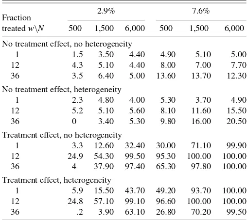
The size and power of the 5% nominal level double-sided Wald tests are displayed in Table 2. When 2.9% of the eligi-bles are treated, the Wald tests perform satisfactory. The tests are significantly undersized for smallNandw, but the size im-proves withN.The power increases withNfor allw’s both with and without heterogeneity. When the fraction treated is 7.6%, the general result is that the actual size is much too large for all
N’s; that the power is not monotonic inwis related to the fact that the treatment effect is significantly smaller atw=36 than atw=12. Thus the variance is underestimated (i.e., we over-state the information in the data) when ignoring the covariance. We have heuristically stated that when the number of treated is small, this would be a possible approach; however, in this set-ting the error involved is large when 7.6% of the population is treated. Note that whenw=1, we estimate only a one-period-ahead effect, and there is no covariance between the survival functions. This is also reflected in Table 2 whenw=1, the real size, is correct for the matching estimator.
Table 1. Bias of the aggregated estimator (%)
Fraction treatedw\N
2.9% 7.6%
500 1,500 6,000 500 1,500 6,000
No treatment effect, no heterogeneity
1 −.09 −.06 .09 −.01 −.01 .02
In our Monte Carlo simulation, we have considered only the performance of the aggregated estimator. The estimator condi-tioning on a particular entry point,s, performs well in all of the different configurations that we consider. The aggregated esti-mator has a very slight bias when there is heterogeneity (2–3% in the worst case). When performing inference, we ignored a covariance stemming from the fact that individuals may enter the survival function as nontreated or as treated. Heuristically, we argued that if the number of treated is small compared with the number of never-treated, then simply ignoring the covari-ance is a viable approach. The Monte Carlo concurs with the argument; this procedure works fine when the sample size is as small as 500, at least when the fraction of treated is 2.9% of the
Table 2. Size and power of the aggregated estimator (%)
Fraction treatedw\N
2.9% 7.6%
500 1,500 6,000 500 1,500 6,000
No treatment effect, no heterogeneity
1 1.5 3.50 4.40 4.90 5.10 5.00
eligible population, but is less viable when the fraction treated is 7.6%.
It should be stressed that the aggregated estimator (13) is of little use if the fraction of treated is large, because then it is generally possible to use the estimator that conditions ons. But if the fraction of treated is low, then sample size may not permit tests for a treatment effect for givens, and then inference using the aggregate estimator may be a good alternative.
5. AN EMPIRICAL APPLICATION
In this section we evaluate the effects of an ES program us-ing the estimators proposed in Section 3. The ES program was administered by the Swedish PES. The prime objective of the PES is to provide the unemployed with job search assistance; a secondary objective is to provide training and subsidized em-ployment. To receive unemployment insurance (UI) or cash as-sistance (CA), the unemployed need to register at the PES; thus all long-term unemployed are registered at the PES. As a way to monitor the unemployed, officials at the PES may require that the unemployed either take a job or take part in a training pro-gram or subsidized employment. If an unemployed individual refuses, then she or he may lose his UI or CA.
The ES program was introduced on January 1, 1998; Fors-lund et al. (2004) have provided a thorough description of the program. The subsidy was targeted at the long-term unem-ployed, that is, individuals registered as unemployed at the PES for at least 12 months. The subsidy amounted to 50% of the to-tal wage costs and was paid for a maximum period of 6 months. We use unemployment register data from the National Labour Market Board, which contains information on all indi-viduals registering at the PES in Sweden since August 1991. The database includes information on, among other factors, age, educational attainment, and sex, as well as the individu-als’ registration date, job training activities, and starting dates of participation in various labor market programs.
For each individual registered at the PES, we observe an event history including the number of spells and days of un-employment. We drop all individuals who left the register be-fore the introduction of the ES program from the data set. We also exclude all individuals for whom the first spell of unem-ployment occurred before January 1, 1992 and for whom all registered spells were shorter than 365 days. The reason for the last two exclusions is that previous labor market history is the key variable for the matching estimator, and the main eligibil-ity criteria for the program is continuous unemployment for at least 365 days.
We focus on individuals age 25 to 63 years at the time of registration at the PES. We chose the lower age limit because eligibility conditions were changed for individuals under age 25. We impose the upper age limit because retirement is im-minent for individuals above age 63 years. A spell of unem-ployment is defined as an uninterrupted period of time during which an unemployed person is registered at the PES. The spell is ended if the unemployed person has a job for a period of at least 30 days or leaves the register for a period of at least 30 days for any other reason. We thus aggregate the daily data to monthly intervals. We do this for two reasons. The first reason is measurement error regarding the exact day of the start of a
job spell. The main cause of this measurement error is the strat-egy used by PES officers for obtaining the information on when the job spell began. If the unemployed individual has not been in contact with the PES office for some specific time period, the individual is asked over the phone whether or not she or he is employed. The second reason is that we want to ameliorate an-ticipation effects. The no-anan-ticipation assumption requires that the individual knows neither the exact date of the program start nor the exact date of a start of a job spell. This is a much more plausible assumption at the monthly interval than at the daily frequency.
It is possible to have more than one spell of unemployment of at least 365 days without interruption while the ES program has been running. Thus an individual can be eligible for the pro-gram more than once. The unit of observation is chosen to be every time that an individual becomes eligible for the ES pro-gram. In the analysis, we use information on each individual’s total number of spells and total days of unemployment before becoming eligible for the ES. For an individual who is eligible more than once, the total number of days and spells is updated each time he or she becomes eligible. Thus the data include only persons who have been eligible for the ES program on at least one occasion.
The individuals in the data are separated into two different groups: those who start the ES program after having become eligible and eligibles who do not start the program. Each time that a person becomes eligible, the total number of days until he or she either leaves the PES office or becomes right-censored is calculated. The point in time for right-censoring is October 1, 2002 or when a person leaves the register for another destina-tion than work. For those who enter the ES program, the dura-tion to ES is calculated as well.
A total of 631,358 individuals, age 25–63, were eligible for ES between January 1998 and October 2002; 3% of the eligible spells ended in ES. The mean characteristics of the ES partici-pants and nonparticipartici-pants in the eligible population are reported in Table 3.
A significantly higher fraction (64% compared with 39%) of the ES spells ended up in employment. This does not indicate a positive treatment effect; to some extent, it reflects the fact that the program participants on average registered earlier at the PES (seeT0) and thus on average had spent a longer time look-ing for a job. Males and non-Nordic immigrants are overrep-resented and disabled individuals are underrepoverrep-resented among the participants. Participants are younger, more educated, and have spent less time at the PES before the last period of unem-ployment. Given reasonable priors about how these character-istics should influence the exit to employment, the participants should be expected to leave unemployment more rapidly than the nonparticipants.
To apply our estimators in the present setting, we must check whether selection on observables is a reasonable assumption. To make a long story short, we believe that these assumption are palatable in the present setting; nonetheless, we attempt to substantiate this claim somewhat.
In a stated preference experiment, Eriksson (1997) found that the heterogeneity of the PES caseworker was more important than the heterogeneity of the individuals in determining pro-gram participation. Carling and Richardson (2004) reported ev-idence in the same vein. They compared the effects of eight
Table 3. Mean characteristics of participants (ES), nonparticipants (no ES), and exactly matched sample (matched)
ES, No ES, ES–No ES, Matched,
Variable mean mean t-value mean
Duration, months 34.38 23.37 62.90
Employed .64 .39 71.54
Covariates
Male .61 .41 56.38 .56
Non-Nordic .21 .14 25.41 .14
No UI .16 .18 −5.43 .11
Disabled .06 .10 −20.41 .02 Upper-secondary degree .43 .35 24.08 .42 University degree .12 .12 −3.43 .09
Age≤30 .26 .22 11.34 .24
30<age≤40 .32 .31 3.39 .30 40<age≤50 .27 .24 7.04 .25
Days in register during previous spell (TD)
TD=0 .41 .38 9.44 .51
0<TD≤100 .05 .05 4.28 .02 100<TD≤500 .22 .20 8.37 .19 500<TD≤1000 .18 .18 1.22 .15
Number of previous programs (TP)
TP=0 .41 .38 7.15 .51
0<TP≤5 .42 .39 7.82 .35 5<TP≤15 .17 .22 −18.62 .14
Month turning eligible (T0) (January 1998=1; October 2002=118)
T0 58.33 70.22 −65.75 60.18
different programs on the probability of finding a job and found that their results did not reflect selection by demonstrating that program placement depended more on the employment service office that the job seeker had visited than on his or her observed characteristics.
It may well be that individual unobserved characteristics are correlated with the PES office. Thus, ideally we would like to control for the PES office in our analysis. This is not possible, however; instead, we control for local labor market in the analy-sis. The local labor market and the PES office overlap to some extent; at the time, there were 100 local labor markets (defined on the basis of commuting patterns) and about 300 PES offices. For the specific ES program that we consider, there also is survey evidence on the selection process (see Lundin 2000). The survey was directed to the caseworkers at the PES. The most important piece of evidence is that only 6% maintained that the initiative to suggest ES came from the eligible, sug-gesting that individual self-selection to ES is not a big problem. Nevertheless, unobserved heterogeneity may remain an issue if caseworkers have more information about the unemployed than we do. However, Eriksson (1997) showed that caseworkers cat-egorize the motivation of identical unemployed individuals very differently, suggesting that this is not so problematic. Moreover, we have detailed information on the previous labor market his-tory (presumably a good indicator of motivation/skills), and we can control for the local labor market in which the individual is registered.
Another threat to the selection on observables assumption stems from the amount of information possessed by the unem-ployed. We must assume that the unemployed knows neither
the exact date of entering ES nor the exact date of starting a job; there must be some randomness in these events. The ex-piration of UI benefits may be considered a violation of this assumption; however, this is not true. Because the expiration of UI occurs at the same time point for all unemployed with the same unemployment duration, the hazards to ES or work are affected in the same way for all unemployed.
We match on the covariates listed in Table 3 and the local labor market in which the individual is registered. In this ap-plication, we use a one-to-one exact matching estimator. Exact matching implies that the common support restriction signifi-cantly reduces the sample (a 60% reduction). An alternative is to use a propensity score-matching estimator (see the App. and Fredriksson and Johansson 2003 for an application). Propen-sity score-matching increases the efficiency of the estimators— because it is easier to find a match—but also may introduce bias. In this particular application, a propensity score-matching approach has no implications for the results.
Index the treated ats=0, . . . ,L−1 byiand the comparison group atsbyc. The unique match (for eachs) is then given by
ci=xi≡xc, c∈N(s), (15) where N(s) is the number of individuals in the comparison group. If there is more than one individual in the comparison group with the same values of the covariates, then we random-ize over the potential matches. If no unique match fromcis found for individual i, then this individual is removed from the estimation. With complete pairs of treated and nontreated individuals, (13) is estimated using the difference in Kaplan– Meier survival function if treated and nontreated for the sub-set of treated individuals with support common to the compar-ison sample. Matching is based on 7,651 treated individuals. Descriptive statistics for the matched pairs are given in Table 3.
5.1 Results
In this application, there is a sufficient number of treated indi-viduals to compute treatment effects by pretreatment duration; see (9) and (10). Figure 2(c) plots the treatment effect for those entering during months 0–3 after eligibility, (b) plots the treat-ment effect for those entering during months 36–39, and (a)
Figure 2. Treatment effects for early and late entrants [ , 95% confidence interval; , difference (36≤t≤39); , difference (0≤t≤3)]
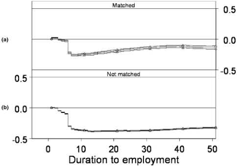
Figure 3. Treatment effects for all entrants: (a) matched; (b) not matched ( , difference; , 95% confidence interval).
shows the treatment effects in the same graph. The increased variance of the estimates in (b) is due to the fact that there were only 206 treated individuals on the common support. The gen-eral message is that treatment effects are similar irrespective of the timing of program entry. A formal Kolmogorov–Smirnov test of equality of the two distributions substantiates this con-clusion; the test has ap-value of .48.
Because there is no evidence suggesting that treatment ef-fects vary by pretreatment duration, we move on to the aggre-gate estimator (13). Figure 3 shows the results. The confidence intervals are calculated using the approximate covariance es-timator (14). In this application this is a good approximation because the fraction treated is small (3%); furthermore, only 256 of the 7,651 treated individuals are included in the set of comparison individuals earlier on.
Figure 3(a) shows the result when controlling for both pre-ES duration and covariates, whereas the estimate in the (b) con-trols only for pre-ES duration. This means that the difference between (a) and (b) reflects the effects of observed heterogene-ity (including the common support restriction). These results indicate that individuals with favorable characteristics are more likely to participate in the ES program.
From Figure 3, we can see that after an initial period of about 6 months with a negligible (negative) treatment effect, a down-ward jump occurs; from then on, the effect gradually becomes smaller, but it is significant over the remainder of the follow-up horizon. This scenario is consistent with an initial period of locking-in and a subsequent period with a positive treatment ef-fect. The sum of the effects over the entire follow-up horizon is 7.78 months, which thus implies that unemployment duration decreased by 14% over the follow-up horizon for the average individual.
A likely explanation for the downward jump in the estimated treatment effect after 6 months is that the participants simply tend to stay on at the workplace where they were employed with the subsidy. On the one hand, this is an intended effect of the program, on the other hand, this result may be seen as an indication that the program tends to displace regular employ-ment; that is, employers use the subsidy to fill vacancies that would have been filled by hiring on the regular market in the absence of the program. The qualitative evidence reported by Lundin (2000) is consistent with this interpretation.
6. CONCLUDING REMARKS
In this article we have considered the evaluation problem us-ing observational data when the start of treatment is the out-come of a stochastic process. We have shown that the duration framework in discrete time (with a time-varying treatment in-dicator) is a fertile ground for effect evaluations. A treatment effect estimator that is based on a static treatment indicator in-variably will be biased.
We have suggested easy-to-use nonparametric matching es-timators of the survival functions. These eses-timators do not rely on strong assumptions about the functional forms of the two processes generating the inflow into programs and employment. We have assumed that selection is based purely on observables. Whether or not the conditional independence assumptions re-quired for the estimators are reasonable depends crucially on the richness of the information in the data. But even if we as-sume that unobserved heterogeneity is not an issue, the evalu-ation problem is demanding on the data. We need longitudinal data from which we can observe the duration path. Knowing the entire path is crucial, because we need to define a compar-ison sample that is matched in terms of the pretreatment dura-tion.
We have demonstrated the usefulness of the estimator using a small Monte Carlo simulation and an application. The estima-tors that we propose conveniently estimate the time profile of treatment effects. This is valuable because the estimated time profile gives vital information on the effects of the program on treated individuals.
In the application considered—the evaluation of an ES program—we found evidence of locking-in effects during the first 6 months after program entry. After 6 months (the maxi-mum duration of the program), there was a big downward jump in the employment hazard, which persisted for the entire follow-up period. Therefore, our overall conclusion is that the program had a positive effect on employment for treated individuals.
We have presented two versions of our estimator, one that conditions on a particular entry point and another that aggre-gates these effects over all entry points. The first estimator con-veys valuable information on the targeting of the program, that is, it answers such questions as whether or not the program should be offered primarily early during an unemployment spell. The aggregated estimator is more pertinent to the ques-tion of whether or not in general more treatment slots should be made available. In the present application, we found that the treatment effects did not vary much by pretreatment duration; thus there is no evidence suggesting that one particular form of targeting is more efficient than another.
We believe that the issues that we have raised apply fairly generally. Considering the evaluations of labor market pro-grams, the problems associated with estimating well-defined treatment effects affect all outcomes that are functions of the outflow to employment. Thus our estimator applies directly when the outcome of interest is employment (or annual earn-ings) some time after the start of a program. Moreover, if skill loss increases with unemployment duration, as suggested by the recent analysis of Edin and Gustavsson (2004), then care should be taken when estimating the effect of treatment on wages.
ACKNOWLEDGMENTS
The authors thank the associate editor, two anonymous refer-ees, as well as Kenneth Carling, Markus Frölich, Paul Frijters, Xavier de Luna, Jeffrey Smith, and Gerard van den Berg for very useful comments. Comments from seminar participants at the conference on “The Evaluation of Labour Market Policies” (Amsterdam, October 2002), Department of Statistics, Umeå University, and IFAU are also gratefully acknowledged. Finan-cial support was provided by the Swedish Council for Working Life and Social Research (FAS).
APPENDIX: MATCHING WITH COVARIATES
Here we devise a matching estimator for the more realis-tic case with observed heterogeneity. Denote by xs the
ob-served covariates for the population treated at s, and define
e(xs)=Pr(D(s)=1|xs)as the conditional probability for the
population at risk of being treated at s given xs. Then it is
straightforward to show the following result.
Proposition A.1. IfW0(s)⊥⊥D(s)|xsande(xs) <1 for allxs,
then the counterfactual survival function for the average treated individual,F0(w,s), can be estimated using individuals who are nontreated atsand have covariatesxs.
Proof. If
W0(s)⊥⊥D(s)|xs, ∀s, (A.1)
then
{Y0(w,s)}∞w=1⊥⊥D(s)|xs, ∀s (A.2)
in discrete time. Assume further that
e(xs) <1, ∀xs. (A.3)
Given (A.1) and (A.3), and assuming random censoring, we have
maining in) unemployment atwgiven nontreatment atsfor the sample of individuals with covariatesxsand Ex
s is the expecta-tion with respect toxs. By (A.2), it holds that (see Rosenbaum
and Rubin 1983)
which justifies matching based on the propensity score.
Under the conditions laid out in Proposition A.1,
x(w,s)=ExsF1xs(w,s)−F0xs(w,s)
(A.4)
is an unbiased estimator of the effects of treatment by entry duration.
To aggregate over pretreatment durations, we can use
χ0(w)=EsEx|s
tuskats, and covariatesxs, who are still at risk and unemployed
inw.
[Received May 2004. Revised May 2007.]
REFERENCES
Abadie, A., and Imbens, G. (2002), “Simple and Bias-Corrected Matching Es-timators for Average Treatment Effects,” Technical Working Paper 283, Na-tional Bureau of Economic Research.
(2006), “On the Failure of the Bootstrap for Matching Estimators,” Technical Working Paper 325, National Bureau of Economic Research. Abbring, J., and van den Berg, G. (2003), “The Non-Parametric Identification
of Treatment Effects in Duration Models,”Econometrica, 71, 1491–1518. Carling, K., and Richardson, K. (2004), “The Relative Efficiency of Labor
Mar-ket Programs: Swedish Experience From the 1990s,”Labour Economics, 11, 335–354.
Dawid, A. (1979), “Conditional Independence in Statistical Theory,”Journal of the Royal Statistical Society, Ser. B, 41, 1–31.
Edin, P.-A., and Gustavsson, M. (2004),“Time Out of Work and Skill Depreci-ation,” Working Paper 2004:14, Uppsala University, Dept. of Economics. Eriksson, M. (1997), “Placement of Unemployed Into Labour Market
Pro-grams: A Quasi-Experimental Study,” Economic Studies 439, Umeå Uni-versity.
Forslund, A., Johansson, P., and Lindquist, L. (2004), “Employment Subsidies: A Fast Lane From Unemployment to Work?” Working Paper 2004:18, Insti-tute for Labour Market Policy Evaluation.
Fredriksson, P., and Johansson, P. (2003), “Employment, Mobility, and Active Labor Market Programs,” Working Paper 2003:5, Uppsala University, Dept. of Economics.
(2004), “Dynamic Treatment Assignment: The Consequences for Evaluations Using Observational Data,” Discussion Paper 1062, IZA. Gerfin, M., and Lechner, M. (2002), “A Microeconometric Evaluation of the
Active Labour Market Policy in Switzerland,”Economic Journal, 112, 854– 893.
Greenwood, M. (1926),A Report on the Natural Duration of Cancer: Appen-dix I:The “Errors of Sampling” of the Survivorship Tables: Reports on Pub-lic Health and Medical Subjects, London: His Majesty’s Stationery Office, London.
Heckman, J., Lalonde, R., and Smith, J. (1999), “The Economics and Econo-metrics of Active Labor Market Programs,” inHandbook of Labor Eco-nomics, Vol. 3, eds. O. Ashenfelter and D. Card, Amsterdam: North-Holland, pp. 1865–2097.
Imbens, G. (2004), “Nonparametric Estimation of Average Treatment Effects Under Exogeneity: A Review,”The Review of Economics and Statistics, 86, 4–29.
Kaplan, E., and Meier, P. (1958), “Nonparametric Estimation From Incomplete Observations,”Journal of the American Statistical Association, 53, 457–481. Lechner, M. (1999), “Earnings and Employment Effects of Continuous Off-the-Job Training in East Germany After Unification,”Journal of Business & Economic Statistics, 17, 74–90.
(2004), “Sequential Matching Estimation of Dynamic Causal Models,” Discussion Paper 2004-06, University of St. Gallen, Dept. of Economics. Lundin, M. (2000), “Anställningsstödens Implementering vid
Arbetsförmedlin-garna,” Stencilserie 2000:4, Institute for Labour Market Policy Evaluation. Richardson, K., and van den Berg, G. (2001), “The Effect of Vocational
Em-ployment Training on the Individual Transition Rate From UnemEm-ployment to Work,”Swedish Economic Policy Review, 8, 175–213.
Robins, J. (1986), “A New Approach to Causal Inference in Mortality Stud-ies With Sustained Exposure Periods: Application to Control of the Healthy Worker Survivor Effect,”Mathematical Modelling, 7, 1393–1512. Rosenbaum, P., and Rubin, D. (1983), “The Central Role of the Propensity
Score in Observational Studies for Causal Effect,”Biometrika, 70, 41–55. van den Berg, G., van der Klaauw, B., and van Ours, J. (2004), “Punitive
Sanc-tions and the Transition Rate From Welfare to Work,”Journal of Labor Eco-nomics, 22, 211–241.
![Figure 2. Treatment effects for early and late entrants [, 95%(0confidence interval;, difference (36 ≤ ≤ t ≤ 39);, difference t ≤ 3)]](https://thumb-ap.123doks.com/thumbv2/123dok/1113485.759793/9.594.31.281.68.370/figure-treatment-effects-entrants-condence-interval-difference-difference.webp)