Full Terms & Conditions of access and use can be found at
http://www.tandfonline.com/action/journalInformation?journalCode=ubes20
Download by: [Universitas Maritim Raja Ali Haji] Date: 11 January 2016, At: 22:45
Journal of Business & Economic Statistics
ISSN: 0735-0015 (Print) 1537-2707 (Online) Journal homepage: http://www.tandfonline.com/loi/ubes20
Out-of-Sample Forecast Tests Robust to the Choice
of Window Size
Barbara Rossi & Atsushi Inoue
To cite this article: Barbara Rossi & Atsushi Inoue (2012) Out-of-Sample Forecast Tests Robust
to the Choice of Window Size, Journal of Business & Economic Statistics, 30:3, 432-453, DOI: 10.1080/07350015.2012.693850
To link to this article: http://dx.doi.org/10.1080/07350015.2012.693850
Published online: 20 Jul 2012.
Submit your article to this journal
Article views: 437
View related articles
Out-of-Sample Forecast Tests Robust
to the Choice of Window Size
Barbara R
OSSIDepartment of Economics, Pompeu Fabra University, ICREA, CREI Barcelona GSE, Barcelona 08019, Spain
([email protected];[email protected])
Atsushi I
NOUEDepartment of Agricultural and Resource Economics, North Carolina State University, Raleigh, NC 27695-8109
This article proposes new methodologies for evaluating economic models’ out-of-sample forecasting performance that are robust to the choice of the estimation window size. The methodologies involve evaluating the predictive ability of forecasting models over a wide range of window sizes. The study shows that the tests proposed in the literature may lack the power to detect predictive ability and might be subject to data snooping across different window sizes if used repeatedly. An empirical application shows the usefulness of the methodologies for evaluating exchange rate models’ forecasting ability.
KEY WORDS: Estimation window; Forecast evaluation; Predictive ability testing.
1. INTRODUCTION
This article proposes new methodologies for evaluating the out-of-sample forecasting performance of economic models. The novelty of the methodologies we propose is that they are robust to the choice of the estimation and evaluation window size. The choice of the estimation window size has always been a concern for practitioners, since the use of different window sizes may lead to different empirical results in practice. In ad-dition, arbitrary choices of window sizes have consequences about how the sample is split into in-sample and out-of-sample portions. Notwithstanding the importance of the problem, no satisfactory solution has been proposed so far, and in the fore-casting literature, it is common to only report empirical results for one window size. For example, to illustrate the differences in the window sizes, we draw on the literature on forecasting exchange rates (the empirical application we will focus on): Meese and Rogoff (1983a) used a window size of 93 obser-vations in monthly data, Chinn (1991) used a window size of 45 in quarterly data, Qi and Wu (2003) used a window size of 216 observations in monthly data, Cheung, Chinn, and Pascual (2005) considered window sizes of 42 and 59 observations in quarterly data, Clark and West (2007) used a window size of 120 observations in monthly data, Gourinchas and Rey (2007) considered a window size of 104 observations in quarterly data, and Molodtsova and Papell (2009) considered a window size of 120 observations in monthly data. This common practice raises two concerns. A first concern is that the “ad-hoc” window size used by the researcher may not detect significant predictive abil-ity even if there would be significant predictive abilabil-ity for some other window size choices. A second concern is the possibil-ity that satisfactory results were obtained simply by chance, after data snooping over window sizes. That is, the successful evidence in favor of predictive ability might have been found after trying many window sizes, although only the results for the successful window size were reported and the search pro-cess was not taken into account when evaluating their statistical
significance. Only rarely do researchers check the robustness of the empirical results to the choice of the window size by reporting results for a selected choice of window sizes. Ulti-mately, however, the size of the estimation window is not a parameter of interest for the researcher: the objective is rather to test predictive ability and, ideally, researchers would like to reach empirical conclusions that are robust to the choice of the estimation window size.
This article views the estimation window as a “nuisance pa-rameter”: we are not interested in selecting the “best” window; rather, we would like to propose predictive ability tests that are “robust” to the choice of the estimation window size. The pro-cedures we propose ensure that this is the case, by evaluating the models’ forecasting performance for a variety of estima-tion window sizes and then taking summary statistics of this sequence. Our methodology can be applied to most tests of pre-dictive ability that have been proposed in the literature, such as Diebold and Mariano (1995), West (1996), McCracken (2000), and Clark and McCracken (2001). We also propose method-ologies that can be applied to Mincer and Zarnowitz’s (1969) tests of forecast efficiency, as well as to more general tests of forecast optimality. Our methodologies allow for both rolling-and recursive-window estimation schemes rolling-and let the window size to be large relative to the total sample size. Finally, we also discuss methodologies that can be used in the Giacomini and White (2005) and Clark and West (2007) frameworks, where the estimation scheme is based on a rolling window of fixed size.
This article is closely related to the works by Pesaran and Timmermann (2007) and Clark and McCracken (2009), and more distantly related to Pesaran, Pettenuzzo, and Timmer-mann (2006) and Giacomini and Rossi (2010). Pesaran and Timmermann (2007) proposed cross-validation and forecast
© 2012American Statistical Association Journal of Business & Economic Statistics
July 2012, Vol. 30, No. 3 DOI:10.1080/07350015.2012.693850
432
combination methods that identify the “ideal” window size using sample information. In other words, Pesaran and Timmer-mann (2007) extended forecast-averaging procedures to deal with the uncertainty over the size of the estimation window, for example, by averaging forecasts computed from the same model but over various estimation window sizes. Their main objective was to improve the model’s forecast. Similarly, Clark and McCracken (2009) combined rolling and recursive forecasts in an attempt to improve the forecasting model. Our article instead proposes to take summary statistics of tests of predictive ability computed over several estimation window sizes. Our objective is neither to improve the forecasting model nor to estimate the ideal window size. Rather, our objective is to assess the robust-ness of conclusions of predictive ability tests to the choice of the estimation window size. Pesaran, Pettenuzzo, and Timmermann (2006) exploited the existence of multiple breaks to improve forecasting ability; to do so, they needed to estimate the process driving the instability in the data. An attractive feature of the procedure we propose is that it does not need to impose or determine when the structural breaks happened. Giacomini and Rossi (2010) proposed techniques to evaluate the relative performance of competing forecasting models in unstable environments, assuming a “given” estimation window size. In this article, our goal is instead to ensure that forecasting ability tests are robust to the choice of the estimation window size. That is, the procedures we propose in this article are designed to determine whether findings of predictive ability are robust to the choice of the window size, not to determine at which point in time the predictive ability shows up: the latter is a very different issue, important as well, and has been discussed in Giacomini and Rossi (2010). Finally, this article is linked to the literature on data snooping: if researchers report empirical results for just one window size (or a couple of them) when they actually considered many possible window sizes prior to reporting their results, their inference will be incorrect. This article provides a way to account for data snooping over several window sizes and removes the arbitrary decision of the choice of the window size. After the first version of this article was submitted, we became aware of an independent work by Hansen and Timmermann (2012). Hansen and Timmermann (2012) pro-posed a sup-type test similar to ours, although they focused on p-values of the Diebold and Mariano (1995) test statistic estimated via a recursive-window estimation procedure for nested mod-els’ comparisons. They provided analytic power calculations for the test statistic. Our approach is more generally applicable: it can be used to draw inference on models’ out-of-sample forecast comparisons and to test forecast optimality where the estimation scheme can be rolling recursive fixed, fixed-window estimation scheme can be either a fixed fraction of the total sample size or fi-nite. Also, Hansen and Timmermann (2012) did not consider the effects of time-varying predictive ability on the power of the test. We show the usefulness of our methods in an empirical anal-ysis. The analysis reevaluates the predictive ability of models of exchange rate determination by verifying the robustness of the recent empirical evidence in favor of models of exchange rate determination (e.g., Engel, Mark, and West2007; Molodtsova and Papell2009) to the choice of the window size. Our results reveal that the forecast improvements found in the literature are much stronger when allowing for a search over several win-dow sizes. As shown by Pesaran and Timmermann (2005), the
choice of the window size depends on the nature of the possible model instability and the timing of the possible breaks. In partic-ular, a large window is preferable if the data-generating process (DGP) is stationary, but this comes at the cost of lower power, since there are fewer observations in the evaluation window. Similarly, a shorter window may be more robust to structural breaks, although it may not provide as precise an estimation as larger windows if the data generating process is stationary. The empirical evidence shows that instabilities are widespread for exchange rate models (see Rossi2006), which might justify why in several cases, we find improvements in economic mod-els’ forecasting ability relative to the random walk for small window sizes.
The article is organized as follows. Section 2 proposes a framework for tests of predictive ability when the window size is a fixed fraction of the total sample size. Section3presents tests of predictive ability when the window size is a fixed constant relative to the total sample size. Section4shows some Monte Carlo evidence on the performance of our procedures in small samples, and Section5presents the empirical results. Section6 concludes.
2. ROBUST TESTS OF PREDICTIVE ACCURACY WHEN THE WINDOW SIZE IS LARGE
Let h≥1 denote the (finite) forecast horizon. We assume that the researcher is interested in evaluating the performance of h-steps-ahead direct forecasts for the scalar variableyt+husing a vector of predictors xt using a rolling-, recursive-, or fixed-window direct forecast scheme. We assume that the researcher hasPout-of-sample predictions available, where the first pre-diction is made based on an estimate from a sample 1,2, . . . , R
such that the last out-of-sample prediction is made based on an estimate from a sample ofT −R+1, . . . , R+P −1=T, whereR+P +h−1=T +his the size of the available sam-ple. The methods proposed in this article can be applied to out-of-sample tests of equal predictive ability, forecast rationality, and unbiasedness.
To present the main idea underlying the methods proposed in this article, let us focus on the case where researchers are interested in evaluating the forecasting performance of two competing models: model 1, involving parameters θ, and model 2, involving parametersγ. The parameters can be esti-mated with a rolling-, fixed-, or recursive-window estimation scheme. In the rolling-window forecast method, the model’s true but unknown parameters θ∗andγ∗ are estimated byθt,R andγt,R, respectively, using samples ofR observations dated
t−R+1, . . . , t, for t=R, R+1, . . . , T. In the recursive-window estimation method, the model’s parameters are instead estimated using samples of t observations dated 1, . . . , t, for
t =R, R+1, . . . , T. In the fixed-window estimation method, the model’s parameters are estimated only once using observa-tions dated 1, . . . , R. Let{L(1)t+h(θt,R)}T
t=R and{L (2)
t+h(γt,R)}Tt=R denote the sequence of loss functions of models 1 and 2 evaluat-ingh-steps-ahead relative out-of-sample forecast errors, respec-tively, and let{Lt+h(θt,R,γt,R)}Tt=Rdenote their difference.
Typically, researchers rely on the Diebold and Mari-ano (1995), West (1996), McCracken (2000), or Clark and McCracken (2001) test statistics for drawing inference on the forecast error loss differences. For example, in the case of the
Diebold and Mariano (1995) and West (1996) tests, researchers evaluate the two models using the sample average of the se-quence of standardized out-of-sample loss differences:
LT(R)≡
Ris a consistent estimate of the long-run variance matrix of the out-of-sample loss differences, which differs between the Diebold and Mariano (1995) and the West (1996) approach.
The problem we focus on is that inference based on Equa-tion (1) relies crucially on R, which is the size of the rolling window in the rolling estimation scheme or the way the sam-ple is split into the in-samsam-ple and out-of-samsam-ple portions in the fixed and recursive estimation schemes. In fact, any out-of-sample test for inference regarding predictive ability does require researchers to chooseR. The problem we focus on is that it is possible that, in practice, the choice ofRmay affect the empirical results. Our main goal is to design procedures that will allow researchers to make inference about predictive ability in a way that does not depend on the choice of the window size. We argue that the choice ofRraises two types of concerns. First, if the researcher tries several window sizes and then reports the empirical evidence based on the window size that provides him the best empirical evidence in favor of predictive ability, his test may be oversized. That is, the researcher will reject the null hypothesis of equal predictive ability in favor of the alternative that the proposed economic model forecasts the best too often, thus finding predictive ability even if it is not significant in the data. The problem is that the researcher is effectively “data-mining” over the choice ofRand does not correct the critical values of the test statistic to take into account the search over window sizes. This is mainly a size problem.
A second type of concern arises when the researcher has simply selected an ad-hoc value ofRwithout trying alternative values. In this case, it is possible that, when there is some pre-dictive ability only over a portion of the sample, he or she may lack empirical evidence in favor of predictive ability because the window size was either too small or too large to capture it. This is mainly a lack of power problem.
Our objective is to considerRas a nuisance parameter and de-velop test statistics to draw inference about predictive ability that does not depend onR. The main results in this article follow from a very simple intuition: if partial sums of the test function (fore-cast error losses, adjusted fore(fore-cast error losses, or functions of forecast errors) obey a functional central limit theorem (FCLT), then we can take any summary statistic across window sizes to robustify inference and derive its asymptotic distribution by applying the continuous mapping theorem (CMT). We consider two appealing and intuitive types of weighting schemes over the window sizes. The first scheme is to choose the largest value of theLT(R) test sequence, which corresponds to a “sup-type” test. This mimics the case of a researcher experimenting with a variety of window sizes and reporting only the empirical re-sults corresponding to the best evidence in favor of predictive ability. The second scheme involves taking a weighted average of the LT(R) tests, giving equal weight to each test. This choice is appropriate when researchers have no prior informa-tion on which window sizes are the best for their analysis. This
choice corresponds to an average-type test. Alternative choices of weighting functions could be entertained and the asymptotic distribution of the resulting test statistics could be obtained by arguments similar to those discussed in this article.
The following proposition states the general intuition behind the approach proposed in this article. In the subsequent subsec-tions, we will verify that the high-level assumption in Proposi-tion 1, EquaProposi-tion (2), holds for the test statistics we are interested in.
Proposition 1 (Asymptotic distribution). LetST(R) denote a test statistic with window sizeR. We assume that the test statistic
ST(·) we focus on satisfies
ST([ι(·)T]) ⇒ S(·), (2)
whereι(·) is the identity function, that is,ι(x)=x and⇒ de-notes weak convergence in the space of cadlag functions on [0,1] equipped with the Skorokhod metric. Then,
sup
Note that this approach assumes thatRis growing with the sample size and, asymptotically, becomes a fixed fraction of the total sample size. This assumption is consistent with the approaches by West (1996), West and McCracken (1998), and McCracken (2000). The next section will consider test statistics where the window size is fixed. Note also that based on Propo-sition 1, we can construct both one-sided and two-sided test statistics; for example, as a corollary of the proposition, one can construct two-sided test statistics in the “sup-type” test statistic by noting that sup[µT]≤R≤[µT]|ST(R)|
d
→supµ≤µ≤µ|S(µ)|, and similarly of the average-type test statistic.
In the existing tests,µ=limT→∞RT is fixed and condition (2) holds pointwise for a givenµ. Condition (2) requires that the convergence holds uniformly in µ rather than pointwise, however. It turns out that this high-level assumption can be shown to hold for many of the existing tests of interest under their original assumptions. As we will show in the next subsections, this is because existing tests had already imposed assumptions for the FCLT to take into account recursive, rolling, and fixed estimation schemes and because weak convergence to stochastic integrals can hold for partial sums (Hansen1992).
Note also that the practical implementation of (3) and (4) requires researchers to chooseµandµ. To avoid data snooping over the choices ofµandµ, we recommend researchers to im-pose symmetry by fixingµ=1−µand to useµ=[0.15] in practice. The recommendation is based on the small-sample per-formance of the test statistics we propose, discussed in Section4. We next discuss how this result can be directly applied to widely used measures of relative forecasting performance, where the loss function is the difference of the forecast er-ror losses of two competing models. We consider two separate cases, depending on whether the models are nested or nonnested. Subsequently, we present results for regression-based tests
of predictive ability, such as Mincer and Zarnowitz’s (1969) forecast rationality regressions, among others. For each of the cases we consider, Appendix A provides a sketch of the proof that the test statistics satisfy condition (2), provided the variance estimator converges in probability uniformly inR. Our proofs are a slight modification of West (1996), Clark and McCracken (2001), and West and McCracken (1998) and extend their re-sults to weak convergence in the space of functions on [µ, µ]. The uniform convergence of variance estimators follows from the uniform convergence of second moments of summands in the numerator and the uniform convergence of rolling and re-cursive estimators, as in the literature on structural change (see Andrews1993, for example).
2.1 Nonnested Models’ Comparisons
Traditionally, researchers interested in drawing inference about the relative forecasting performance of competing, nonnested models rely on the Diebold and Mariano (1995), West (1996) and McCracken (2000) test statistics. The statistic tests the null hypothesis that the expected value of the loss dif-ferences evaluated at the pseudo-true parameter values equals zero. That is, letL∗T(R) denote the value of the test statistic evaluated at the true parameter values; then, the null hypothesis can be rewritten as:E[L∗T(R)]=0 . The test statistic that they propose relies on the sample average of the sequence of standardized out-of-sample loss differences, Equation (1):
LT(R)≡
whereσR2is a consistent estimate of the long-run variance matrix of the out-of-sample loss differences. A consistent estimate of
σ2for nonnested models’ comparisons that does not take into account parameter estimation uncertainty is provided in Diebold and Mariano (1995). Consistent estimates of σ2that take into account parameter estimation uncertainty in recursive windows are provided by West (1996), and in rolling and fixed windows, are provided by McCracken (2000, p. 203, eqs. (5) and (6)). For example, a consistent estimator when parameter estimation error is negligible is P (e.g., Newey and West1987). In particular, a leading case where (6) can be used is when the same loss function is used for estimation and evaluation. For convenience, we provide the consistent variance estimate for rolling, recursive, and fixed estimation schemes in Appendix A.
Appendix A shows that Proposition 1 applies to the test statis-tic (5) under broad conditions. Examples of typical nonnested models satisfying Proposition 1 (provided that the appropriate moment conditions are satisfied) include linear and nonlinear models estimated by any extremum estimator [e.g., ordinary
least squares (OLS), general method of moments (GMM), and maximum likelihood estimator (MLE)]; the data can have serial correlation and heteroscedasticity, but are required to be sta-tionary under the null hypothesis (which rules out unit roots and structural breaks). McCracken (2000) showed that this frame-work allows for a wide class of loss functions.
Our proposed procedure specialized to two-sided tests of nonnested forecast models’ comparisons is as follows. Let
RT = sup
R is a consistent estimator of σ 2.
Re-Researchers might be interested in performing one-sided tests as well. In that case, the tests in Equations (7) and (8)
Finally, it is useful to remind readers that, as discussed in Clark and McCracken (2011b), Equation (5) is not necessarily asymptotically normal even when the models are not nested. For example, whenyt+1=α0+α1xt+ut+1 andyt+1=β0+ β1zt+vt+h, with xt independent of zt and α1=β1=0, the two models are nonnested but (5) is not asymptotically normal. The asymptotic normality result does not hinge on whether or
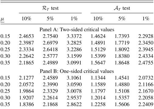
Table 1. Critical values for nonnested models’ comparisons
RT test AT test
µ 10% 5% 1% 10% 5% 1%
Panel A: Two-sided critical values
0.15 2.4653 2.7540 3.3372 1.4624 1.7393 2.2928 0.20 2.3987 2.6979 3.2825 1.4891 1.7719 2.3450 0.25 2.3334 2.6418 3.2286 1.5129 1.8092 2.3945 0.30 2.2642 2.5777 3.1599 1.5399 1.8380 2.4334 0.35 2.1865 2.4989 3.0991 1.5647 1.8648 2.4755
Panel B: One-sided critical values
0.15 2.1277 2.4589 3.1061 1.1344 1.4541 2.0732 0.20 2.0572 2.3990 3.0590 1.1589 1.4880 2.1166 0.25 1.9864 2.3329 3.0078 1.1797 1.5108 2.1670 0.30 1.9207 2.2614 2.9537 1.2014 1.5357 2.2058 0.35 1.8386 2.1868 2.8622 1.2258 1.5606 2.2409
NOTE:µis the fraction of the smallest window size relative to the sample size,µ= limT→∞(R/T). The critical values are obtained by Monte Carlo simulation using 50,000 Monte Carlo replications in which Brownian motions are approximated by normalized partial sums of 10,000 standard normal random variates.
not two models are nested but rather on whether or not the disturbance terms of the two models are numerically identical in population under the null hypothesis.
2.2 Nested Models’ Comparison
For the case of nested models’ comparison, we follow Clark and McCracken (2001). Let model 1 be the parsimonious model and model 2 be the larger model that nests model 1. Letyt+h denote the variable to be forecast and let the period-tforecasts of yt+hfrom models 1 and 2 be denoted byy1,t+h andy2,t+h, respectively: the first (“small”) model usesk1regressorsx1,tand the second (“large”) model usesk1+k2=kregressorsx1,tand
x2,t. Clark and McCracken’s (2001) ENCNEW test is defined as
wherePis the number of out-of-sample predictions available, andy1,t+h,y2,t+hdepend on the parameter estimates ˆθt,R,γˆt,R. Note that, since the models are nested, Clark and McCracken’s (2001) test is one-sided.
Appendix A shows that Proposition 1 applies to the test statis-tic (9) under the same assumptions as in Clark and McCracken (2001). In particular, their assumptions hold for one-step-ahead forecast errors (h=1) from linear, homoscedastic models, OLS estimation, and mean squared error (MSE) loss function (as dis-cussed in Clark and McCracken (2001), the loss function used for estimation has to be the same as the loss function used for evaluation).
Our robust procedure specialized to tests of nested forecast models’ comparisons is as follows. Let
RET = sup all R at the significance level α against the alternative HA: limT→∞E[LET(R)]>0 for someRwhenR
α,where the critical values k
R
α andk
A
α for µ=0.15 are re-ported in Table 2(a) for the rolling-window estimation scheme, and in Table 2(b) for the recursive-window estimation scheme.
2.3 Regression-Based Tests of Predictive Ability
Under the widely used mean squared forecast error (MSFE) loss, optimal forecasts have a variety of properties. They should be unbiased, one-step-ahead forecast errors should be serially uncorrelated, andh-steps-ahead forecast errors should be cor-related at most of orderh−1 (see Granger and Newbold1986 and Diebold and Lopez1996). It is therefore interesting to test such properties. We do so in the same framework as West and McCracken’s (1998). Let the forecast error evaluated at the pseudo-true parameter valuesθ∗bevt+h(θ∗)≡vt+h, and its
es-in the les-inear relationship between the prediction error,vt+h, and a (p×1) vector function of data at timet.
For the purposes of this section, let us define the loss func-tion of interest to beLt+h(θ), whose estimated counterpart is
Lt+h(θt,R)≡Lt+h. To be more specific, we give its definition. Definition (Special cases of regression-based tests of pre-dictive ability). The following are special cases of regression-based tests of predictive ability: (a)Forecast unbiasedness tests:
Lt+h=vt+h.(b)Mincer–Zarnowitz’s (1969) tests(or efficiency tests):Lt+h=vt+hXt, whereXtis a vector of predictors known at time t (see also Chao, Corradi, and Swanson 2001). One important special case is whenXtis the forecast itself. (c) Fore-cast encompassing tests(Chong and Hendry 1986, Clements and Hendry 1993, Harvey, Leybourne, and Newbold 1998):
Lt+h=vt+hft, where ft is the forecast of the encompassed model. (d)Serial uncorrelation tests:Lt+h=vt+hvt.
More generally, let the loss function of interest be the (p×1) vector Lt+h(θ∗)=vt+hgt, whose estimated counter-part isLt+h=vt+hgt, wheregt(θ∗)≡gt denotes the function describing the linear relationship betweenvt+h and a (p×1) vector function of data at timet, withgt(θt)≡gt. In the exam-ples above: (a)gt =1, (b)gt =Xt, (c)gt =ft, and (d)gt =vt. The null hypothesis of interest is typically:
E(Lt+h(θ∗))=0. (12)
To test (12), one simply tests whetherLt+hhas zero mean by a
standard Wald test in a regression ofLt+honto a constant (i.e.,
testing whether the constant is zero). That is,
WT(R)=P−1
whereRis a consistent estimate of the long-run variance ma-trix of the adjusted out-of-sample losses,, typically obtained by using West and McCracken’s (1998) estimation procedure.
Appendix A shows that Proposition 1 applies to the test statistic (13) under broad conditions, which are similar to those discussed for Equation (5). The framework allows for linear and nonlinear models estimated by any extremum estimator (e.g., OLS, GMM, and MLE), the data to have serial correlation and heteroscedasticity as long as stationarity is satisfied (which rules out unit roots and structural breaks), and forecast errors (which can be either one-period errors or multiperiod errors) evaluated using continuously differentiable loss functions, such as the MSE.
Our proposed procedure specialized to tests of forecast opti-mality is as follows. Let
RWT = sup
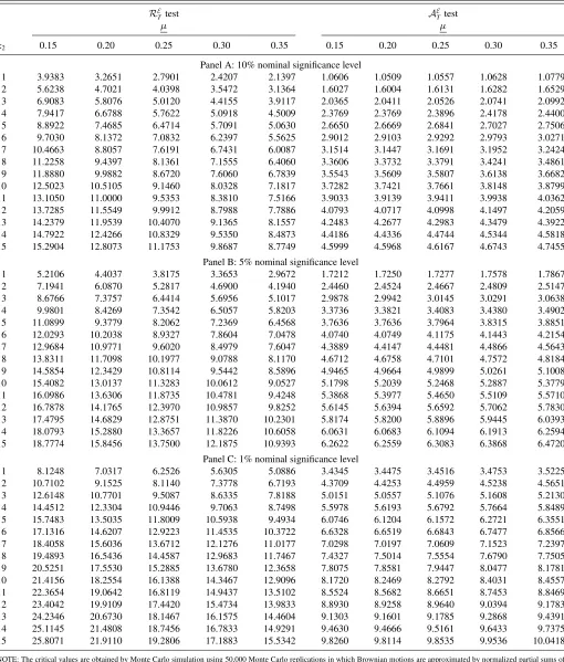
Table 2(a). Critical values for nested models’ comparisons using ENCNEW in rolling regressions
RE
Ttest A
E
T test
µ µ
k2 0.15 0.20 0.25 0.30 0.35 0.15 0.20 0.25 0.30 0.35
Panel A: 10% nominal significance level
1 3.9383 3.2651 2.7901 2.4207 2.1397 1.0606 1.0509 1.0557 1.0628 1.0779 2 5.6238 4.7021 4.0398 3.5472 3.1364 1.6027 1.6004 1.6131 1.6282 1.6529 3 6.9083 5.8076 5.0120 4.4155 3.9117 2.0365 2.0411 2.0526 2.0741 2.0992 4 7.9417 6.6788 5.7622 5.0918 4.5009 2.3769 2.3769 2.3896 2.4178 2.4400 5 8.8922 7.4685 6.4714 5.7091 5.0630 2.6650 2.6669 2.6841 2.7027 2.7506 6 9.7030 8.1372 7.0832 6.2397 5.5625 2.9012 2.9103 2.9292 2.9793 3.0271 7 10.4663 8.8057 7.6191 6.7431 6.0087 3.1514 3.1447 3.1691 3.1952 3.2424 8 11.2258 9.4397 8.1361 7.1555 6.4060 3.3606 3.3732 3.3791 3.4241 3.4861 9 11.8880 9.9882 8.6720 7.6060 6.7839 3.5543 3.5609 3.5807 3.6138 3.6682 10 12.5023 10.5105 9.1460 8.0328 7.1817 3.7282 3.7421 3.7661 3.8148 3.8799 11 13.1050 11.0000 9.5353 8.3810 7.5166 3.9033 3.9139 3.9411 3.9938 4.0362 12 13.7285 11.5549 9.9912 8.7988 7.7886 4.0793 4.0717 4.0998 4.1497 4.2059 13 14.2379 11.9539 10.4070 9.1365 8.1557 4.2483 4.2677 4.2983 4.3479 4.3922 14 14.7922 12.4266 10.8329 9.5350 8.4873 4.4186 4.4336 4.4744 4.5344 4.5818 15 15.2904 12.8073 11.1753 9.8687 8.7749 4.5999 4.5968 4.6167 4.6743 4.7455
Panel B: 5% nominal significance level
1 5.2106 4.4037 3.8175 3.3653 2.9672 1.7212 1.7250 1.7277 1.7578 1.7867 2 7.1941 6.0870 5.2817 4.6900 4.1940 2.4460 2.4524 2.4667 2.4809 2.5147 3 8.6766 7.3757 6.4414 5.6956 5.1017 2.9878 2.9942 3.0145 3.0291 3.0638 4 9.9801 8.4269 7.3542 6.5057 5.8203 3.3736 3.3821 3.4083 3.4380 3.4902 5 11.0899 9.3779 8.2062 7.2369 6.4568 3.7636 3.7636 3.7964 3.8315 3.8851 6 12.0293 10.2038 8.9327 7.8604 7.0478 4.0740 4.0749 4.1175 4.1443 4.2154 7 12.9684 10.9771 9.6020 8.4979 7.6047 4.3889 4.4147 4.4481 4.4866 4.5643 8 13.8311 11.7098 10.1977 9.0788 8.1170 4.6712 4.6758 4.7101 4.7572 4.8184 9 14.5854 12.3429 10.8114 9.5442 8.5896 4.9465 4.9664 4.9899 5.0261 5.1008 10 15.4082 13.0137 11.3283 10.0612 9.0527 5.1798 5.2039 5.2468 5.2887 5.3779 11 16.0986 13.6306 11.8735 10.4781 9.4248 5.3868 5.3977 5.4650 5.5109 5.5710 12 16.7878 14.1765 12.3970 10.9857 9.8252 5.6145 5.6394 5.6592 5.7062 5.7830 13 17.4795 14.6829 12.8751 11.3870 10.2301 5.8174 5.8200 5.8896 5.9445 6.0393 14 18.0793 15.2880 13.3657 11.8226 10.6058 6.0631 6.0683 6.1094 6.1913 6.2594 15 18.7774 15.8456 13.7500 12.1875 10.9393 6.2622 6.2559 6.3083 6.3868 6.4720
Panel C: 1% nominal significance level
1 8.1248 7.0317 6.2526 5.6305 5.0886 3.4345 3.4475 3.4516 3.4753 3.5225 2 10.7102 9.1525 8.1140 7.3778 6.7193 4.3709 4.4253 4.4959 4.5238 4.5651 3 12.6148 10.7701 9.5087 8.6335 7.8188 5.0151 5.0557 5.1076 5.1608 5.2130 4 14.4512 12.3304 10.9446 9.7063 8.7498 5.5978 5.6193 5.6792 5.7664 5.8489 5 15.7483 13.5035 11.8009 10.5938 9.4934 6.0746 6.1204 6.1572 6.2721 6.3551 6 17.1316 14.6207 12.9223 11.4535 10.3722 6.6328 6.6519 6.6843 6.7477 6.8566 7 18.4058 15.6036 13.6712 12.1276 11.0177 7.0298 7.0197 7.0609 7.1523 7.2397 8 19.4893 16.5436 14.4587 12.9683 11.7467 7.4327 7.5014 7.5554 7.6790 7.7505 9 20.5251 17.5530 15.2885 13.6780 12.3658 7.8075 7.8581 7.9447 8.0477 8.1781 10 21.4156 18.2554 16.1388 14.3467 12.9096 8.1720 8.2469 8.2792 8.4031 8.4557 11 22.3654 19.0642 16.8119 14.9437 13.5102 8.5524 8.5682 8.6651 8.7453 8.8469 12 23.4042 19.9109 17.4420 15.4734 13.9833 8.8930 8.9258 8.9640 9.0394 9.1783 13 24.2346 20.6730 18.1467 16.1575 14.4604 9.1303 9.1601 9.1785 9.2868 9.4391 14 25.1145 21.4808 18.7456 16.7833 14.9291 9.4630 9.4666 9.5161 9.6433 9.7375 15 25.8071 21.9110 19.2806 17.1883 15.5342 9.8260 9.8114 9.8535 9.9536 10.0418
NOTE: The critical values are obtained by Monte Carlo simulation using 50,000 Monte Carlo replications in which Brownian motions are approximated by normalized partial sums of 10,000 standard normal random variates.k2is the number of additional regressors in the nesting model.
and R is a consistent estimator of . Reject the null hy-pothesis H0 : limT→∞E(Lt+h(θ∗))=0 for all R at the sig-nificance level α when RWT > kR
α for the sup-type test and when AWT > kA,W
α,p for the average-type test, where the
crit-ical values kR,W
α,p and k
A,W
α,p for µ=0.15 are reported in Table 3.
A simple, consistent estimator forcan be obtained by fol-lowing the procedures in West and McCracken (1998). West
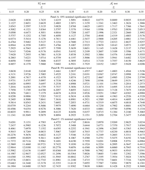
Table 2(b). Critical values for nested models’ comparisons using ENCNEW in recursive regressions
RE
T test A
E
Ttest
µ µ
k2 0.15 0.20 0.25 0.30 0.35 0.15 0.20 0.25 0.30 0.35
Panel A: 10% nominal significance level
1 2.0428 1.8830 1.7435 1.6219 1.5091 0.8622 0.8775 0.8889 0.9035 0.9145 2 3.1227 2.8651 2.6639 2.4803 2.3071 1.3159 1.3341 1.3463 1.3624 1.3886 3 3.8543 3.5597 3.3135 3.0828 2.8768 1.6625 1.6933 1.7117 1.7366 1.7641 4 4.5082 4.1321 3.8364 3.5797 3.3376 1.9164 1.9396 1.9763 2.0036 2.0513 5 5.0500 4.6473 4.3051 4.0016 3.7208 2.1657 2.1996 2.2321 2.2660 2.3092 6 5.5757 5.1252 4.7305 4.4050 4.1127 2.3704 2.4048 2.4319 2.4803 2.5176 7 6.0374 5.5414 5.1276 4.7811 4.4461 2.5437 2.5800 2.6205 2.6861 2.7341 8 6.4764 5.9482 5.5127 5.1154 4.7680 2.7313 2.7723 2.8313 2.8637 2.9257 9 6.8944 6.3558 5.8931 5.4766 5.1087 2.9325 2.9670 3.0143 3.0573 3.1207 10 7.2925 6.7043 6.1977 5.7599 5.3639 3.0651 3.1145 3.1628 3.2137 3.2765 11 7.6143 7.0246 6.5176 6.0541 5.6192 3.2109 3.2607 3.3109 3.3586 3.4171 12 7.9420 7.2955 6.7881 6.3120 5.8538 3.3502 3.3884 3.4376 3.4948 3.5555 13 8.2883 7.6221 7.0714 6.5759 6.1197 3.5006 3.5339 3.5941 3.6482 3.7235 14 8.6058 7.9305 7.3606 6.8337 6.3895 3.6514 3.7110 3.7557 3.8150 3.8825 15 8.8857 8.1370 7.5860 7.0482 6.5921 3.7525 3.8152 3.8827 3.9428 4.0206
Panel B: 5% nominal significance level
1 3.0638 2.8140 2.6240 2.4461 2.2837 1.4557 1.4647 1.4803 1.4944 1.5156 2 4.3131 3.9726 3.7085 3.4525 3.2181 2.0191 2.0367 2.0747 2.0998 2.1306 3 5.2001 4.7817 4.4370 4.1523 3.8574 2.4272 2.4667 2.4985 2.5294 2.5799 4 5.9751 5.4797 5.0997 4.7538 4.4246 2.7898 2.8346 2.8649 2.9151 2.9672 5 6.6020 6.0993 5.6497 5.2538 4.8908 3.0721 3.1101 3.1594 3.2014 3.2573 6 7.2016 6.6383 6.1759 5.7537 5.3856 3.3314 3.3874 3.4495 3.5145 3.5688 7 7.7958 7.1705 6.6788 6.2057 5.8055 3.6212 3.6614 3.7128 3.7675 3.8320 8 8.3056 7.6811 7.1379 6.6678 6.2018 3.8526 3.9251 3.9847 4.0383 4.0988 9 8.8298 8.0886 7.5283 7.0132 6.5634 4.1026 4.1468 4.1963 4.2526 4.3328 10 9.2405 8.5008 7.8841 7.3616 6.8901 4.2921 4.3589 4.4014 4.4695 4.5361 11 9.5814 8.8543 8.2431 7.6692 7.2053 4.4731 4.5319 4.6075 4.6818 4.7440 12 10.0759 9.2244 8.5686 7.9979 7.4890 4.6464 4.7230 4.7902 4.8681 4.9279 13 10.4586 9.6354 8.9276 8.3086 7.7620 4.8333 4.8881 4.9780 5.0596 5.1334 14 10.8035 9.9911 9.2899 8.6125 8.0456 5.0157 5.0715 5.1384 5.2180 5.3065 15 11.1341 10.3049 9.5879 8.8894 8.2925 5.1351 5.2050 5.2704 5.3477 5.4548
Panel C: 1% nominal significance level
1 5.6201 5.1151 4.7583 4.4755 4.1745 2.8616 2.8970 2.9269 2.9625 3.0234 2 7.2437 6.5985 6.1236 5.7072 5.3488 3.6444 3.6771 3.7370 3.7917 3.8304 3 8.4061 7.6970 7.1352 6.6393 6.2252 4.1941 4.2496 4.2845 4.3363 4.3943 4 9.5015 8.7269 8.0833 7.5067 7.0207 4.7015 4.7737 4.8230 4.8818 4.9463 5 10.2276 9.3676 8.6622 8.1127 7.5346 5.1724 5.2169 5.2603 5.3311 5.4173 6 11.0099 10.0029 9.3611 8.6827 8.1067 5.4380 5.4751 5.5475 5.6192 5.7446 7 11.7372 10.7116 9.9961 9.1691 8.6190 5.7559 5.8201 5.8908 5.9751 6.0984 8 12.3869 11.4660 10.5721 9.7422 9.1030 6.1524 6.2224 6.2895 6.3647 6.4412 9 12.9844 12.0180 11.1165 10.2776 9.6076 6.4368 6.5099 6.6060 6.7043 6.7516 10 13.5982 12.6136 11.6897 10.8368 10.0149 6.7008 6.7982 6.9033 6.9543 7.0391 11 14.1987 12.9637 12.0527 11.2496 10.5364 7.0026 7.0685 7.1484 7.2302 7.3586 12 14.6368 13.3992 12.4392 11.5945 10.8842 7.2767 7.3195 7.3934 7.5024 7.5876 13 15.0736 13.8831 12.7743 11.8981 11.2180 7.4715 7.5770 7.6601 7.7316 7.8259 14 15.6463 14.3440 13.3178 12.3353 11.6119 7.6955 7.7587 7.8581 7.9879 8.1301 15 16.1904 14.8480 13.7635 12.7435 11.9302 7.9630 8.0681 8.1428 8.2522 8.3688
NOTE: The critical values are obtained by Monte Carlo simulation using 50,000 Monte Carlo replications in which Brownian motions are approximated by normalized partial sums of 10,000 standard normal random variates.k2denotes the number of additional regressors in the nesting forecasting model.
and McCracken (1998) showed that it is very important to allow for a general variance estimator that takes into account estima-tion uncertainty and/or correcting the statistics by the necessary adjustments (see West and McCracken’s (1998) table 2 for
de-tails on the necessary adjustment procedures for correcting for parameter estimation uncertainty). The same procedures should be implemented to obtain correct inference in regression-based tests in our setup. For convenience, we discuss in detail how to
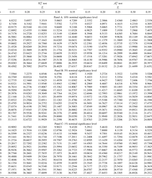
Table 3(a). Critical values for regression-based forecast tests in rolling regressions
RW
T test A
W
T test
µ µ
p 0.15 0.20 0.25 0.30 0.35 0.15 0.20 0.25 0.30 0.35
Panel A: 10% nominal significance level
1 6.0232 5.6957 5.3519 5.0603 4.7289 2.3352 2.3866 2.4360 2.4863 2.5356 2 8.7104 8.3182 7.9441 7.5702 7.1775 4.0327 4.0971 4.1615 4.2310 4.3055 3 10.9175 10.5160 10.1210 9.6689 9.2188 5.5968 5.6865 5.7731 5.8579 5.9555 4 12.8892 12.4355 11.9888 11.5234 11.0328 6.9825 7.1009 7.1930 7.2968 7.4078 5 14.7178 14.2720 13.8253 13.3149 12.8049 8.3948 8.5133 8.6385 8.7684 8.8849 6 16.5061 16.0064 15.5135 14.9935 14.4440 9.6853 9.8289 9.9636 10.1149 10.2460 7 18.2076 17.6931 17.1643 16.6285 16.0431 10.9867 11.1379 11.3069 11.4364 11.5806 8 19.8602 19.2927 18.7560 18.1639 17.5679 12.2381 12.4036 12.5735 12.7378 12.9106 9 21.4528 20.8269 20.2910 19.7234 19.0474 13.5190 13.6791 13.8281 13.9988 14.1684 10 23.0218 22.3889 21.8070 21.1754 20.5231 14.7707 14.9352 15.0980 15.3045 15.4487 11 24.4742 23.8423 23.2744 22.6039 21.9323 15.9558 16.1214 16.2999 16.4800 16.6643 12 26.0187 25.3868 24.7328 24.0608 23.3456 17.1518 17.3281 17.5026 17.6942 17.8671 13 27.5256 26.8514 26.1987 25.5138 24.8065 18.4130 18.5986 18.7856 18.9767 19.1441 14 29.0283 28.3664 27.6849 27.0006 26.2935 19.6634 19.8409 20.0041 20.2057 20.3971 15 30.4502 29.7092 29.0774 28.4029 27.6317 20.8167 21.0132 21.2140 21.4499 21.6352
Panel B: 5% nominal significance level
1 7.5564 7.2275 6.8546 6.4796 6.0972 3.1920 3.2724 3.3522 3.4358 3.5206 2 10.3769 10.0324 9.6538 9.2701 8.8118 5.1033 5.2112 5.3354 5.4318 5.5503 3 12.7735 12.3460 11.9425 11.4939 11.0302 6.7967 6.9427 7.0852 7.2406 7.3766 4 14.8321 14.3901 13.9540 13.4943 12.9867 8.2969 8.4687 8.6318 8.7958 8.9664 5 16.7614 16.2736 15.8067 15.3362 14.8067 9.7989 9.9693 10.1493 10.3354 10.5375 6 18.5950 18.0767 17.6066 17.1015 16.5707 11.2498 11.4217 11.6045 11.8109 11.9937 7 20.3976 19.8283 19.3049 18.7764 18.2241 12.6046 12.7993 12.9861 13.1972 13.3996 8 22.1168 21.5762 21.1031 20.4959 19.8974 13.9372 14.1526 14.3703 14.5839 14.8045 9 23.8522 23.2566 22.6911 22.1283 21.4786 15.2917 15.5188 15.7380 15.9483 16.1988 10 25.4795 24.9024 24.2752 23.6293 23.0278 16.5691 16.7627 17.0114 17.2422 17.4755 11 27.0374 26.4198 25.7992 25.1407 24.5003 17.8549 18.0967 18.3394 18.5560 18.8105 12 28.6076 27.9345 27.3250 26.7175 26.0002 19.1315 19.3671 19.6241 19.8921 20.1026 13 30.1707 29.5526 28.9241 28.2376 27.4890 20.4014 20.6697 20.9340 21.2116 21.4713 14 31.7441 31.0769 30.4594 29.8000 29.0350 21.7238 21.9949 22.2826 22.5831 22.8479 15 33.3115 32.6722 31.9929 31.2398 30.4675 22.9763 23.2559 23.5206 23.7834 24.0850
Panel C: 1% nominal significance level
1 10.9092 10.5765 10.2265 9.9023 9.4320 5.2912 5.4610 5.6518 5.8473 6.0006 2 14.1825 13.7016 13.3209 12.8796 12.3924 7.6681 7.8800 8.1139 8.3134 8.5258 3 16.5599 16.2327 15.8236 15.4133 14.9400 9.5437 9.7501 10.0145 10.2618 10.4837 4 19.1441 18.5812 18.1744 17.7106 17.2011 11.2408 11.4497 11.7294 12.0478 12.2695 5 21.2724 20.6837 20.2955 19.7587 19.2763 12.8595 13.1439 13.4204 13.7497 14.0333 6 23.2017 22.7202 22.2382 21.7131 21.1407 14.4503 14.7644 15.0760 15.3602 15.7306 7 25.0052 24.5921 24.0584 23.5994 23.0652 15.9616 16.3350 16.7109 16.9853 17.3829 8 26.9436 26.3662 25.9507 25.3262 24.7723 17.5904 17.8867 18.2658 18.5772 18.8987 9 28.7768 28.2601 27.7835 27.1973 26.4835 19.0634 19.4360 19.8217 20.2149 20.5634 10 30.4888 29.9409 29.3264 28.7970 28.1661 20.3842 20.7962 21.1757 21.5661 21.9883 11 32.4046 31.7953 31.2932 30.6334 30.0165 21.8198 22.2137 22.7070 23.0265 23.4243 12 34.1354 33.5681 33.0216 32.4559 31.6939 23.3545 23.7738 24.1897 24.6128 24.9903 13 35.6631 35.0345 34.5340 33.9171 33.2544 24.7177 25.1323 25.5434 25.9649 26.3638 14 37.1971 36.7807 36.3541 35.5661 34.8225 26.0787 26.4930 26.9710 27.4368 27.8999 15 38.9308 38.3865 37.8899 37.3130 36.5785 27.4027 27.8453 28.3305 28.8926 29.2522
NOTE: The critical values are obtained by Monte Carlo simulation using 50,000 Monte Carlo replications in which Brownian motions are approximated by normalized partial sums of 10,000 standard normal random variates.pdenotes the number of restrictions being tested.
construct a consistent variance estimate in the leading case of Mincer and Zarnowitz’s (1969) regressions in rolling, recursive, or fixed estimation schemes in Appendix B.
Historically, researchers have estimated the alterna-tive regression, vt+h=gt′·α(R)+ηt+h, where α(R)=
(P−1Tt=Rgtgt′) −1
(P−1Tt=Rgtvt+h) and ηt+h is the fitted error of the regression, and tested whether the coefficients equal zero. It is clear that under the additional assumption thatE(gtg′t) is full rank (a maintained assumption in the fore-cast rationality literature), the two procedures share the same
Table 3(b). Critical values for regression-based forecast tests in recursive regressions
RW
T test A
W
T test
µ µ
p 0.15 0.20 0.25 0.30 0.35 0.15 0.20 0.25 0.30 0.35
Panel A: 10% nominal significance level
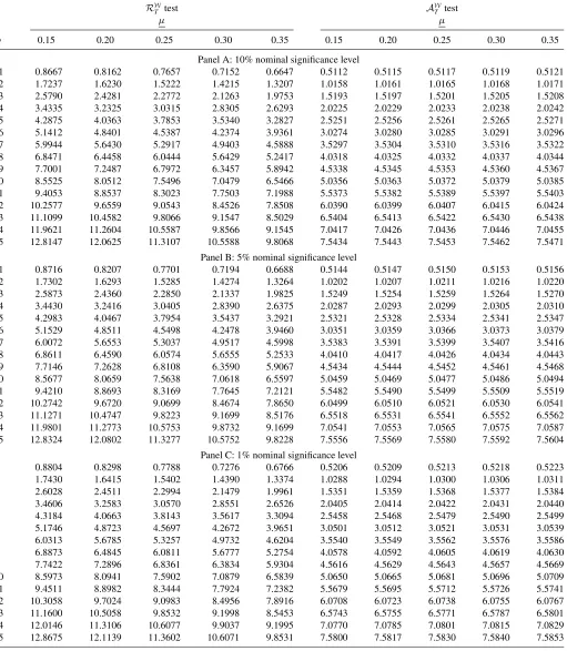
1 0.8667 0.8162 0.7657 0.7152 0.6647 0.5112 0.5115 0.5117 0.5119 0.5121 2 1.7237 1.6230 1.5222 1.4215 1.3207 1.0158 1.0161 1.0165 1.0168 1.0171 3 2.5790 2.4281 2.2772 2.1263 1.9753 1.5193 1.5197 1.5201 1.5205 1.5208 4 3.4335 3.2325 3.0315 2.8305 2.6293 2.0225 2.0229 2.0233 2.0238 2.0242 5 4.2875 4.0363 3.7853 3.5340 3.2827 2.5251 2.5256 2.5261 2.5265 2.5271 6 5.1412 4.8401 4.5387 4.2374 3.9361 3.0274 3.0280 3.0285 3.0291 3.0296 7 5.9944 5.6430 5.2917 4.9403 4.5888 3.5297 3.5304 3.5310 3.5316 3.5322 8 6.8471 6.4458 6.0444 5.6429 5.2417 4.0318 4.0325 4.0332 4.0337 4.0344 9 7.7001 7.2487 6.7972 6.3457 5.8942 4.5338 4.5345 4.5353 4.5360 4.5367 10 8.5525 8.0512 7.5496 7.0479 6.5466 5.0356 5.0363 5.0372 5.0379 5.0385 11 9.4053 8.8537 8.3023 7.7503 7.1988 5.5373 5.5382 5.5389 5.5397 5.5403 12 10.2577 9.6559 9.0543 8.4526 7.8508 6.0390 6.0399 6.0407 6.0415 6.0424 13 11.1099 10.4582 9.8066 9.1547 8.5029 6.5404 6.5413 6.5422 6.5430 6.5438 14 11.9621 11.2604 10.5587 9.8566 9.1545 7.0417 7.0426 7.0436 7.0446 7.0455 15 12.8147 12.0625 11.3107 10.5588 9.8068 7.5434 7.5443 7.5453 7.5462 7.5471
Panel B: 5% nominal significance level
1 0.8716 0.8207 0.7701 0.7194 0.6688 0.5144 0.5147 0.5150 0.5153 0.5156 2 1.7302 1.6293 1.5285 1.4274 1.3264 1.0202 1.0207 1.0211 1.0216 1.0220 3 2.5873 2.4360 2.2850 2.1337 1.9825 1.5249 1.5254 1.5259 1.5264 1.5270 4 3.4430 3.2416 3.0405 2.8390 2.6375 2.0287 2.0293 2.0299 2.0305 2.0310 5 4.2983 4.0467 3.7954 3.5437 3.2921 2.5321 2.5328 2.5334 2.5341 2.5347 6 5.1529 4.8511 4.5498 4.2478 3.9460 3.0351 3.0359 3.0366 3.0373 3.0379 7 6.0072 5.6553 5.3037 4.9517 4.5998 3.5383 3.5391 3.5399 3.5407 3.5416 8 6.8611 6.4590 6.0574 5.6555 5.2533 4.0410 4.0417 4.0426 4.0434 4.0443 9 7.7146 7.2628 6.8108 6.3590 5.9067 4.5434 4.5444 4.5452 4.5461 4.5468 10 8.5677 8.0659 7.5638 7.0618 6.5597 5.0459 5.0469 5.0477 5.0486 5.0494 11 9.4210 8.8693 8.3169 7.7645 7.2121 5.5482 5.5490 5.5499 5.5509 5.5519 12 10.2742 9.6720 9.0699 8.4674 7.8650 6.0499 6.0510 6.0521 6.0530 6.0541 13 11.1271 10.4747 9.8223 9.1699 8.5176 6.5518 6.5531 6.5541 6.5552 6.5562 14 11.9801 11.2773 10.5753 9.8732 9.1699 7.0541 7.0553 7.0565 7.0575 7.0587 15 12.8324 12.0802 11.3277 10.5752 9.8228 7.5556 7.5569 7.5580 7.5592 7.5604
Panel C: 1% nominal significance level
1 0.8804 0.8298 0.7788 0.7276 0.6766 0.5206 0.5209 0.5213 0.5218 0.5223 2 1.7430 1.6415 1.5402 1.4390 1.3374 1.0288 1.0294 1.0300 1.0306 1.0311 3 2.6028 2.4511 2.2994 2.1479 1.9961 1.5351 1.5359 1.5368 1.5377 1.5384 4 3.4606 3.2583 3.0570 2.8551 2.6526 2.0405 2.0414 2.0422 2.0431 2.0440 5 4.3184 4.0663 3.8143 3.5617 3.3094 2.5458 2.5468 2.5479 2.5490 2.5499 6 5.1746 4.8723 4.5697 4.2672 3.9651 3.0501 3.0512 3.0521 3.0531 3.0539 7 6.0313 5.6785 5.3257 4.9732 4.6204 3.5540 3.5549 3.5562 3.5576 3.5586 8 6.8873 6.4845 6.0811 5.6777 5.2754 4.0578 4.0592 4.0605 4.0619 4.0630 9 7.7422 7.2896 6.8361 6.3834 5.9304 4.5616 4.5629 4.5643 4.5657 4.5669 10 8.5973 8.0941 7.5902 7.0879 6.5839 5.0650 5.0665 5.0681 5.0696 5.0709 11 9.4511 8.8982 8.3444 7.7924 7.2382 5.5679 5.5695 5.5712 5.5726 5.5741 12 10.3058 9.7024 9.0983 8.4956 7.8916 6.0708 6.0723 6.0738 6.0755 6.0767 13 11.1600 10.5058 9.8532 9.1998 8.5453 6.5743 6.5755 6.5771 6.5787 6.5801 14 12.0146 11.3106 10.6077 9.9037 9.1995 7.0770 7.0785 7.0801 7.0815 7.0829 15 12.8675 12.1139 11.3602 10.6071 9.8531 7.5800 7.5817 7.5830 7.5840 7.5853
NOTE: The critical values are obtained by Monte Carlo simulation using 50,000 Monte Carlo replications in which Brownian motions are approximated by normalized partial sums of 10,000 standard normal random variates.pdenotes the number of restrictions being tested.
null hypothesis and are therefore equivalent. However, in this case, it is convenient to define the following rescaled Wald test:
WT(r)(R)=α(R)′ Vα−1(R)α(R),
whereVα(R) is a consistent estimate of the asymptotic variance ofα(R),Vα.We propose the following tests:
RWT = sup R∈{R,...,R}
α(R)′ Vα−1(R)α(R) (16)
and
α,p for the sup-type test and whenA α T > k
A,W
α,p for the average-type test. Simulated values ofkR,W
α,p andk
A,W
α,p forµ=0.15 and various values ofpare reported in Table 3.
Under more general specifications for the loss function, the properties of forecast errors previously discussed may not hold. In those situations, Patton and Timmermann (2007) showed that a “generalized forecast error” does satisfy the same properties. The procedures we propose can also be applied to Patton and Timmermann’s (2007) generalized forecast error.
3. ROBUST TESTS OF PREDICTIVE ACCURACY WHEN THE WINDOW SIZE IS SMALL
All the tests considered so far rely on the assumption that the window is a fixed fraction of the total sample size, asymptot-ically. This assumption rules out the tests by Clark and West (2006,2007) and Giacomini and White (2005), which rely on a constant (fixed) window size. Propositions 2 and 3 extend our methodology in these two cases by allowing the window size to be fixed.
First, we will consider a version of Clark and West’s (2006, 2007) test statistics. The Monte Carlo evidence in Clark and West (2006, 2007) and Clark and McCracken (2001, 2005) shows that Clark and West’s (2007) test has power that is broadly comparable with the power of an F-type test of equal MSE. Clark and West’s (2006,2007) test is also popular because it has the advantage of being approximately normal, which per-mits the tabulation of asymptotic critical values applicable under multistep forecasting and conditional heteroscedasticity. Before we get into details, a word of caution: our setup requires strict exogeneity of the regressors, which is a very strong assumption in time-series application. When the window size diverges to infinity, the correlation between the rolling regression estimator and the regressor vanishes even when the regressor is not strictly exogenous. When the window size is fixed relative to the sample size, however, the correlation does not vanish even asymptot-ically when the regressor is not strictly exogenous. When the null model is the no-change forecast model, as required by the original test of Clark and West (2006,2007) when the window size is fixed, the assumption of strict exogeneity can be dropped and our test statistic becomes identical to theirs.
Consider the following nested forecasting models:
yt+h=β1′x1t+e1,t+h, (18) corresponding models’h-steps-ahead forecast errors. Note that, since the models are nested, Clark and West’s (2007) test is one-sided. Under the null hypothesis that β2∗=[β1∗′0′]′, the
“MSPE-adjusted” of Clark and West (2007) can be written as
MSPE-adjusted out, the mean of MSPE-adjusted is nonzero, unlessx1t is null. We consider an alternative adjustment term so that the adjusted loss difference will have zero mean. Suppose thatβ2∗ =[β1∗′0′]′ and thatx2,t is strictly exogenous. Then, we have
Eeˆ12,t+h−eˆ2,t+h
where the fourth equality follows from the null hypothesis,β∗ 2 = [β∗′
1 0′]′, the fifth equality follows from the null thate2,t+h is orthogonal to the information set at timet, and the last equality follows from the strict exogeneity assumption. Thus,φt+h(R)≡
ˆ
e12,t+h(R)−eˆ22,t+h(R)−[ ˆy12,t+h(R)−yˆ22,t+h(R)] has zero mean even whenx1tis not null, provided that the regressors are strictly exogenous.
WhenRis fixed, Clark and West’s adjustment term is valid if the null model is the no-change forecast model, that is,x1t is null. Whenx1tis null, the second term on the right-hand side of Equation (20) is zero even whenx2t is not strictly exogenous, and our adjustment term and theirs become identical.
Proposition 2 (Robust out-of-sample test with fixed win-dow size I). Suppose that: (a) either x1t is null or int; and (d)RandRare fixed constants. Then,
ξR ≡
where is the long-run covariance matrix, =∞j=−∞Ŵj,
where is a consistent estimate of. The null hypothesis is rejected at the significance levelαfor anyRwhenCWT > χr2;α, whereχ2
r;αis the (1−α)th quantile of a chi-square distribution withrdegrees of freedom.
The proof of this proposition follows directly from corollary 24.7 of Davidson (1994, p. 387). Assumption (a) of Preposition 2 is necessary forφt+h(R) to have zero mean and is satisfied under the assumption discussed by Clark and West (x1t is not null) or under the assumption thatx2tis strictly exogenous. The latter assumption is very strong in the applications of interest.
We also consider the Giacomini and White (2005) frame-work. Proposition 3 provides a methodology that can be used to robustify their test for unconditional predictive ability with respect to the choice of the window size.
Proposition 3 (Robust out-of-sample test with fixed win-dow size II). Suppose the assumptions of theorem 4 in Giacomini and White (2005) hold, and that there exists a unique window size R ∈ {R, . . . , R} for which the null hypothesis
RandRare fixed constants, and ˆσR2is a consistent estimator of
σ2. Under the null hypothesis,
GWT →d N(0,1).
The null hypothesis for the GWT test is rejected at the significance level α in favor of the two-sided alternative limT→∞E[LT(θt,R,γt,R)] =0 for anyRwhenGWT > zα/2, wherezα/2is the 100(1−α/2)% quantile of a standard normal distribution.
Note that, unlike the previous cases, in this case, we consider the inf (·) over the sequence of out-of-sample tests rather than the sup (·). The reason why we do so is related to the special nature of Giacomini and White’s (2005) null hypothesis: if their null hypothesis is true for one window size, then it is necessarily false for other window sizes; thus, the test statistic is asymptot-ically normal for the former, but diverges for the others. That is why it makes sense to take the inf (·). Our assumption that the null hypothesis holds only for one value of Rmay sound
peculiar, but the unconditional predictive ability test of Giaco-mini and White (2005) typically implies a unique value ofR, although there is no guarantee that the null hypothesis of Giaco-mini and White (2006) holds in general. For example, consider the case where data are generated from yt =β2∗+et, where der the unconditional version of the null hypothesis, we have
E[yt2+1−(yt+1−R−1jt=t−R+1yj)2] = 0, which in turn im-plies β2∗2−σR2 = 0. Thus, if the null hypothesis holds, then it holds with a unique value ofR. Our proposed test protects applied researchers from incorrectly rejecting the null hypoth-esis by choosing an ad-hoc window size, which is important especially for the Giacomini and White (2006) test, given its sensitivity to data snooping over window sizes.
The proof of Proposition 3 is provided in Appendix A. Note that one might also be interested in a one-sided test where H0: limT→∞E[LT(θt,R,γt,R)]=0 versus the
alter-In this section, we evaluate the small-sample properties of the methods we propose and compare them with the methods existing in the literature. We consider both nested and nonnested models’ forecast comparisons, as well as forecast rationality. For each of these tests under the null hypothesis, we allow for three choices ofµ, one-step-ahead and multistep-ahead forecasts, and multiple regressors of alternative models to see if and how the size of the proposed tests is affected in small samples. We con-sider the no-break alternative hypothesis and the one-time-break alternative to compare the power of our proposed tests with that of the conventional tests. Below, we report rejection frequencies at the 5% nominal significance level to save space.
For the nested models’ forecast comparison, we consider a modification of the DGP (labeled “DGP 1”) that follows Clark and McCracken (2005a) and Pesaran and Timmermann (2007). Let nested models’ forecasts foryt+h:
Model 1 forecast : θ1,tyt (24) Model 2 forecast : γ1,tyt+γ2′,txt+γ3′,tzt,
and both models’ parameters are estimated by OLS in rolling windows of sizeR.We consider several horizons (h) to evaluate how our tests perform at both the short and the long horizons that are typically considered in the literature. We consider several extra regressors (k2) to evaluate how our tests perform as the estimation uncertainty induced by extra regressors increases. Finally, we consider several sample sizes (T) to evaluate how our tests perform in small samples. Under the null hypothesis,dt,T = 0 for allt and we considerh=1,4,8,k2=1,3,5, andT = 50,100,200,500. Under the no-break alternative hypothesis,
dt,T =0.1 ordt,T =0.2 (h=1,k2=1, andT =200). Under the one-time-break alternative hypothesis,dt,T =0.5·I(t ≤τ) forτ ∈ {40,80,120,160}, (h=1,k2=1, andT =200).
For the nonnested models’ forecast comparison, we consider a modification of DGP1 (labeled “DGP2”):
⎛ models’ forecasts foryt+h:
Model 1 forecast : θ1yt+θ2xt (25) Model 2 forecast : γ1yt+γ2′zt,
and both models’ parameters are estimated by OLS in rolling windows of sizeR. Again, we consider several horizons, extra regressors, and sample sizes:h=1,4,8,k2=2,4,6, andT = 50,100,200,500. We use the two-sided version of our test. Note that, for nonnested models withp >1, one might expect that, in finite samples, model 1 would be more accurate than model 2 because model 2 includes extraneous variables. Under the null hypothesis, dt,T =0.5 for all t. Under the no-break alternative hypothesis,dt,T =1 or dt,T =1.5 (h=1,k2=2, andT =200). Under the one-time-break alternative hypothesis,
dt,T =0.5·I(t≤τ)+0.5 for τ ∈ {40,80,120,160} (h=1,
k2=2, andT =200).
“DGP3” is designed for regression-based tests and is a mod-ification of the Monte Carlo design in West and McCracken
(1998). Let
yt+1 = δt,T ·Ip+0.5yt+εt+1, t =1, . . . , T ,
whereyt+1is ap×1 vector andεt+1 iid
∼ N(0p×1, Ip). We gen-erate a vector of variables rather than a scalar because in this design, we are interested in testing whether the forecast error is not only unbiased but also uncorrelated with information avail-able up to timet, including lags of the additional variables in the model. Let y1,t be the first variable in the vector yt. We
For the forecast comparison tests with a fixed window size, we consider the following DGP (labeled “DGP4”):
yt+1 = δRxt+εt+1, t=1, . . . , T ,
where xt andεt+1 are independent and identically distributed standard normal independent of each other. We compare the following two nested models’ forecasts for yt: a first model is a no-change forecast model, for example, the random-walk forecast for a target variable defined in first differences, and the second is a model with the regressor:
Model 1 forecast : 0
Model 2 forecast : δt,Rxt, the null hypothesis in Proposition 3 holds for one of the win-dow sizes,R, we letδR =(R−2)−1/2. The number of Monte Carlo replications is 5000. To ensure that the null hypothesis in Proposition 2 holds, we letδR =δ=0.
The size properties of our test procedures in small samples are first evaluated in a series of Monte Carlo experiments. We report empirical rejection probabilities of the tests we propose at the 5% nominal level. In all experiments except DGP4, we investigate sample sizes where T =50, 100, 200, and 500, and setµ=0.05,0.15,0.25 andµ=1−µ. For DGP4, we let
P =100,200, and 500, and letR=20 or 30 andR=R+5.
Note that in DGP4, we only consider five values ofRsince the window size is small by assumption, which limits the range of values we can consider. Tables4, 5, and 6 report results for the
Rε T andA
ε
T tests for the nested models’ comparison (DGP1), the RT and AT tests for the nonnested models’ comparison
Table 4. Size results of nested models’ comparison tests—DGP1
RE
50 0.093 0.080 0.074 0.085 0.083 0.065 0.036 0.067 0.067 0.064 0.056 0.038 0.057 0.046 100 0.098 0.067 0.061 0.070 0.078 0.069 0.056 0.058 0.058 0.057 0.054 0.051 0.056 0.053 200 0.070 0.063 0.056 0.070 0.065 0.061 0.056 0.054 0.054 0.051 0.059 0.051 0.053 0.054 500 0.058 0.051 0.053 0.066 0.062 0.055 0.052 0.052 0.052 0.053 0.055 0.059 0.047 0.048
NOTE:his the forecast horizon andk2+1 is the number of regressors in the nesting forecasting model. The nominal significance level is 0.05. The number of Monte Carlo replications is 5000 forh=1 and 500 forh >1 when the parametric bootstrap critical values are used, with the number of bootstrap replications set to 199.
Table 5. Size results of nonnested models’ comparison tests—DGP2
RTtest AT test
µ 0.05 0.15 0.25 0.15 0.15 0.15 0.15 0.05 0.15 0.25 0.15 0.15 0.15 0.15
h 1 1 1 4 8 1 1 1 1 1 4 8 1 1
T k 2 2 2 2 2 4 6 2 2 2 2 2 4 6
50 0.010 0.017 0.019 0.000 0.000 0.071 0.375 0.021 0.029 0.031 0.000 0.000 0.038 0.100 100 0.018 0.024 0.023 0.000 0.000 0.058 0.278 0.036 0.039 0.040 0.003 0.000 0.046 0.084 200 0.023 0.029 0.031 0.004 0.000 0.049 0.127 0.040 0.041 0.040 0.013 0.001 0.045 0.060 500 0.031 0.036 0.036 0.024 0.005 0.040 0.064 0.043 0.042 0.044 0.033 0.004 0.046 0.055
NOTE: Here, we consider the two-sided version of our testsRT andAT.his the forecast horizon andkis the number of regressors in the larger forecasting model. The nominal significance level is 0.05. The number of Monte Carlo replications is 5000.
(DGP2), andRW T andA
W
T for the regression-based tests of pre-dictive ability (DGP3), respectively. For the multiple-horizon case, in nested and regression-based inference, we use the heteroscedasticity- and autocorrelation-consistent (HAC) esti-mator with the truncated kernel, bandwidthh−1, and adjust-ment proposed by Harvey, Leybourne, and Newbold (1997), as suggested by Clark and McCracken (2011a, sec.4), and then bootstrap the test statistics using the parametric bootstrap based on the estimated vector autoregressive (VAR) model, as sug-gested by Clark and McCracken (2005b). Note that designs that have the same parameterization do not have exactly the same rejection frequencies since the Monte Carlo experiments are run independently for the various cases we study, and therefore, there are small differences due to simulation noise. The number of Monte Carlo simulations is set to 5000, except that it is set to 500 and the number of bootstrap replications is set to 199 in Tables4and6whenh >1.
Table 4shows that the nested models’ comparison tests (i.e.,
RE
T and A
E
T tests) have good size properties overall. Except for small sample sizes, they perform well even in the multiple-horizon and multiple-regressor cases. Although the effect of the choice ofµbecomes smaller as the sample size grows, theRET
test tends to overreject with smaller values ofµ. TheAE
T test is less sensitive to the choice ofµ. The tests implemented with
µ=0.05 tend to reject the null hypothesis too often when the sample size is small. For the size properties, we recommendµ=
0.15.Table 5shows that the nonnested models’ comparison tests (RTandATtests) also have good size properties, although they tend to be slightly undersized. They tend to be more undersized as the forecast horizon grows, thus suggesting that the test is less reliable for horizons greater than one period. TheRT test
tends to reject too often when there are many regressors (p=6). Note that by showing that the test is significantly oversized in small samples, the simulation results confirm that for nonnested models withp >1, model 1 is more accurate than model 2 in finite samples, as is expected.Table 6shows the size properties of the regression-based tests of predictive ability (RW
T andA W T tests). The tests tend to reject more often as the forecast horizon increases and less often as the number of restrictions increases. Table 7reports empirical rejection frequencies for DGP4. The left panel shows results for theGWTtest, Equation (23), reported in the column labeled “GWT test.” The table shows that our test is conservative when the number of out-of-sample forecastsP is small, but otherwise, it is controlled. Similar results hold for theCWT test discussed in Proposition 2.
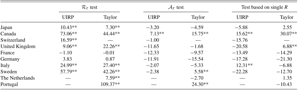
Next, we consider three additional important issues. First, we evaluate the power properties of our proposed procedure in the presence of departures from the null hypothesis in small samples. Second, we show that traditional methods, which rely on an “ad-hoc” window size choice, may have no power at all to detect predictive ability. Third, we demonstrate that traditional methods are subject to data mining (i.e., size distortions) if they are applied to many window sizes without correcting the appropriate critical values.
Tables 8, 9, and 10 report empirical rejection rates for the Clark and McCracken (2001) test under DGP1 withh=1 and
p=0; the nonnested models’ comparison test of Diebold and Mariano (1995), West (1996), and McCracken (2000) under DGP2 with h=1 and p=1; and the West and McCracken (1998) regression-based test of predictive ability under DGP3 withh=1 andp=1, respectively. In each table, the columns labeled “Tests based on singleR” report empirical rejection rates
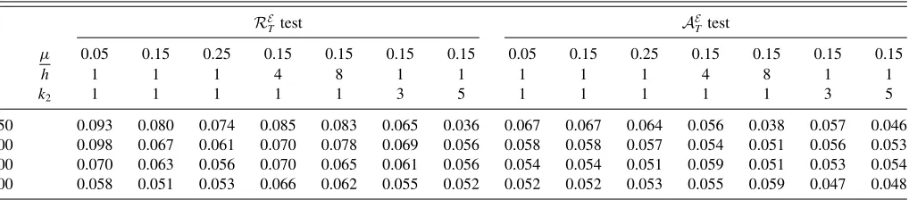
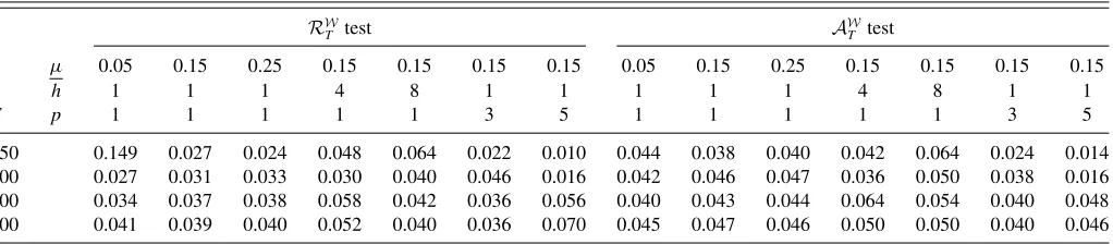
Table 6. Size results of regression-based tests of predictive ability—DGP3
RW
T test A
W
T test
µ 0.05 0.15 0.25 0.15 0.15 0.15 0.15 0.05 0.15 0.25 0.15 0.15 0.15 0.15
h 1 1 1 4 8 1 1 1 1 1 4 8 1 1
T p 1 1 1 1 1 3 5 1 1 1 1 1 3 5
50 0.149 0.027 0.024 0.048 0.064 0.022 0.010 0.044 0.038 0.040 0.042 0.064 0.024 0.014 100 0.027 0.031 0.033 0.030 0.040 0.046 0.016 0.042 0.046 0.047 0.036 0.050 0.038 0.016 200 0.034 0.037 0.038 0.058 0.042 0.036 0.056 0.040 0.043 0.044 0.064 0.054 0.040 0.048 500 0.041 0.039 0.040 0.052 0.040 0.036 0.070 0.045 0.047 0.046 0.050 0.050 0.040 0.046
NOTE:his the forecast horizon andpis the number of restrictions being tested. The nominal significance level is 0.05. The number of Monte Carlo replications is 5000 forh=p=1 and 500 forh >1 orp >1 when the parametric bootstrap critical values are used, with the number of bootstrap replications set to 199.
Table 7. Size results of the fixed window size tests—DGP 4
GWT test CWTtest
P R=20 R=30 R=20 R=30
100 0.0824 0.1140 0.0546 0.0652
200 0.0676 0.0936 0.0460 0.0444
500 0.0362 0.0638 0.0416 0.0480
NOTE: The table reports empirical rejection frequencies of theGWTtest, Equation (23),
implemented withR=20 or 30 andR=R. It also reports empirical rejection frequencies of theCWTtest, Equation (22), implemented with the same choices of window sizes. The
nominal significance level is 0.05. The number of Monte Carlo replications is 5000.
implemented with a specific value ofR, which would correspond to the case of a researcher who has chosen one “ad-hoc” window sizeR, has not experimented with other choices, and thus might have missed predictive ability associated with alternative values ofR. The columns labeled “Data mining” report empirical re-jection rates incurred by a researcher who is searching across all values ofR∈ {30,31, . . . ,170}(“AllR” ) and across five values ofR ∈ {20,40,80,120,160}(“FiveR”). That is, the researcher reports results associated with the most significant window size without taking into account the search procedure when drawing inference. The critical values used for these conventional testing procedures are based on Clark and McCracken (2001) and West and McCracken (1998) for Tables 8 and 10, respectively, and are equal to 1.96 for Table 9. Note that to obtain critical values for the ENCNEW test and regression-based test of predictive ability that are not covered by them, the critical values are estimated from 50,000 Monte Carlo simulations in which the Brownian motion is approximated by normalized partial sums of 10,000 standard normal random variates. For the nonnested models’ comparison test, parameter estimation uncertainty is asymptoti-cally irrelevant by construction and the standard normal critical values can be used. The nominal level is set to 5%, µ=0.15,
µ=0.85, and the sample size is 200.
The first row of each panel reports the size of these test-ing procedures and shows that all tests have approximately the correct size except the data mining procedure, which has size distortions and leads to too many rejections, with probabilities
ranging from 0.175 to 0.253. Even when only five window sizes are considered, data mining leads to falsely rejecting the null hypothesis, with probability more than 0.13. This implies that the empirical evidence in favor of the superior predictive ability of a model can be spurious if evaluated with the incorrect critical values. Panel A of each table shows that the conventional tests and proposed tests have power against the standard no-break alternative hypothesis. Unreported results show that while the power of theRE
T test is increasing inµ, it is decreasing inµfor theRT andRW
T tests. The power of theA
E
T,AT, andAWT tests is not sensitive to the choice ofµ.
Panel B of each table demonstrates that, in the presence of a structural break, the tests based on an “ad-hoc” rolling window size can have low power, depending on the window size and the break location. The evidence highlights the sharp sensitivity of power of all the tests to the timing of the break relative to the forecast evaluation window and shows that, in the presence of instabilities, our proposed tests tend to be more powerful than some of the tests based on an ad-hoc window size, whose power properties crucially depend on the window size. Against the one-time-break alternative, the power of the proposed tests tends to be decreasing in µ. Based on these size and power results, we recommendµ=0.15 in Section2, which provides a good performance overall.
Finally, we show that the effects of data mining are not just a small-sample phenomenon. We quantify the effects of data mining asymptotically by using the limiting distributions of existing test statistics. We design a Monte Carlo simulation where we generate a large sample of data (T = 2000) and use it to construct limiting approximations to the test statis-tics described in Appendix B. For example, in the nonnested models’ comparison case withp=1, the limiting distribution of the Diebold and Mariano (1995) test statistic for a given
µ= lim
T→∞ R
T is (1−µ) −1/2|B
(1)−B(µ)|; the latter can be ap-proximated in large samples by (1−RT)−1/2|P−1/2Tt=Rξt|, where ξt
iid
∼N(0,1). We simulate the latter for many window sizesRand then calculate how many times, on average across 50,000 Monte Carlo replications, the resulting vector of statistics exceeds the standard normal critical values for a 5% nominal
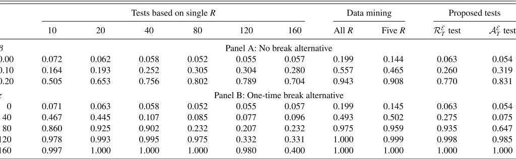
Table 8. Rejection frequencies of nested models’ comparison tests—DGP1
Tests based on singleR Data mining Proposed tests
10 20 40 80 120 160 AllR FiveR RE
T test A
E
Ttest
β Panel A: No break alternative
0.00 0.072 0.062 0.058 0.052 0.055 0.057 0.199 0.144 0.063 0.054
0.10 0.164 0.193 0.252 0.305 0.304 0.280 0.557 0.465 0.260 0.319
0.20 0.505 0.653 0.756 0.802 0.789 0.704 0.943 0.908 0.770 0.831
τ Panel B: One-time break alternative
0 0.071 0.063 0.058 0.052 0.055 0.057 0.199 0.145 0.063 0.054
40 0.467 0.445 0.107 0.085 0.077 0.096 0.493 0.502 0.275 0.075
80 0.860 0.925 0.902 0.232 0.207 0.232 0.975 0.959 0.935 0.647
120 0.978 0.993 0.995 0.975 0.332 0.331 1.000 0.999 0.998 0.985
160 0.997 1.000 1.000 1.000 0.980 0.400 1.000 1.000 1.000 1.000
NOTE:βis the parameter value, withβ=0 corresponding to the null hypothesis.τis the break date, withτ=0 corresponding to the null hypothesis. We seth=1, µ=0.15,µ=0.85, T=200, andp=0. The five values ofRused in the third-last column areR=20,40,80,120,160. The nominal significance level is set to 0.05. The number of Monte Carlo replications is 5000.