Full Terms & Conditions of access and use can be found at
http://www.tandfonline.com/action/journalInformation?journalCode=ubes20
Download by: [Universitas Maritim Raja Ali Haji] Date: 11 January 2016, At: 22:28
Journal of Business & Economic Statistics
ISSN: 0735-0015 (Print) 1537-2707 (Online) Journal homepage: http://www.tandfonline.com/loi/ubes20
Using Heteroscedasticity to Identify and Estimate
Mismeasured and Endogenous Regressor Models
Arthur Lewbel
To cite this article: Arthur Lewbel (2012) Using Heteroscedasticity to Identify and Estimate Mismeasured and Endogenous Regressor Models, Journal of Business & Economic Statistics, 30:1, 67-80, DOI: 10.1080/07350015.2012.643126
To link to this article: http://dx.doi.org/10.1080/07350015.2012.643126
View supplementary material
Published online: 22 Feb 2012.
Submit your article to this journal
Article views: 1282
View related articles
Supplementary materials for this article are available online. Please go tohttp://tandfonline.com/r/JBES
Using Heteroscedasticity to Identify and
Estimate Mismeasured and Endogenous
Regressor Models
Arthur L
EWBELDepartment of Economics, Boston College, 140 Commonwealth Avenue, Chestnut Hill, MA 02467 ([email protected])
This article proposes a new method of obtaining identification in mismeasured regressor models, triangular systems, and simultaneous equation systems. The method may be used in applications where other sources of identification, such as instrumental variables or repeated measurements, are not available. Associated estimators take the form of two-stage least squares or generalized method of moments. Identification comes from a heteroscedastic covariance restriction that is shown to be a feature of many models of endogeneity or mismeasurement. Identification is also obtained for semiparametric partly linear models, and associated estimators are provided. Set identification bounds are derived for cases where point-identifying assumptions fail to hold. An empirical application estimating Engel curves is provided.
KEY WORDS: Endogeneity; Heteroscedastic errors; Identification; Measurement error; Partly linear model; Simultaneous system.
1. INTRODUCTION
This article provides a new method of identifying structural parameters in models with endogenous or mismeasured regres-sors. The method may be used in applications where other sources of identification, such as instrumental variables, re-peated measurements, or validation studies, are not available. The identification comes from having regressors uncorrelated with the product of heteroscedastic errors, which is shown to be a feature of many models in which error correlations are due to an unobserved common factor, such as unobserved abil-ity in returns to schooling models, or the measurement error in mismeasured regressor models. Even when this main identify-ing assumption does not hold, it is still possible to obtain set identification, specifically bounds on the parameters of interest. For the main model, estimators take the form of modified two-stage least squares or generalized method of moments (GMM). Identification of semiparametric partly linear triangular and si-multaneous systems is also considered. In an empirical appli-cation, this article’s methodology is applied to deal with mea-surement error in total expenditures, resulting in Engel curve estimates that are similar to those obtained using a more stan-dard instrument. A literature review shows similarly satisfactory empirical results obtained by other researchers using this arti-cle’s methodology, based on earlier working article versions of this article.
LetY1 andY2 be observed endogenous variables, letXbe a vector of observed exogenous regressors, and letε=(ε1,ε2) be unobserved errors. For now, consider structural models of the form:
Y1 =X′β1+Y2γ1+ε1 (1)
Y2 =X′β2+Y1γ2+ε2. (2)
Later, the identification results will be extended to cases where
X′β1andX′β2are replaced by unknown functions ofX.
This system of equations is triangular whenγ2=0, other-wise it is fully simultaneous (if it is known thatγ1=0, then renumber the equations to setγ2=0). The errorsε1andε2may be correlated with each other.
AssumeE(εX)=0, which is the standard minimal regres-sion assumption for the exogenous regressorsX. This permits identification of the reduced form, but is of course not suf-ficient to identify the structural model coefsuf-ficients. Typically, structural model identification is obtained by imposing equality constraints on some coefficients, such as assuming that some elements ofβ1orβ2are zero, which is equivalent to assuming
the availability of instruments. This article instead obtains iden-tification by restricting correlations ofεε′withX. The resulting
identification is based on higher moments and so is likely to pro-vide less reliable estimates than identification based on standard exclusion restrictions, but may be useful in applications where traditional instruments are not available or could be used along with traditional instruments to increase efficiency.
Restricting correlations ofεε′withXdoes not automatically
provide identification. In particular, the structural model param-eters remain unidentified under the standard homoskedasticity assumption thatE(εε′|X) is constant, and more generally, are not identified whenεandXare independent.
However, what this article shows is that the model parameters may be identified given some heteroscedasticity. In particular, identification is obtained by assuming that cov(X, ε2
j)=0 for
j =2 in a triangular system (or for bothj =1 andj =2 in a fully simultaneous system) and assuming that cov(Z, ε1ε2)=
0 for an observed Z, where Z can be a subset of X. If
cov(Z, ε1ε2)=0, then set identification, specifically bounds on
© 2012American Statistical Association Journal of Business & Economic Statistics January 2012, Vol. 30, No. 1 DOI:10.1080/07350015.2012.643126
67
parameters, can still be obtained as long as this covariance is not too large.
The remainder of this section provides examples of models where these identifying assumptions hold and comparisons to related results in the literature.
1.1 Independent Errors
For the simplest possible motivating example, let Equations (1) and (2) hold. Suppose ε1 andε2 have the standard model error property of being mean zero and are conditionally in-dependent of each other, so ε1 ⊥ ε2|Z and E(ε1)=0. It would then follow immediately that the key identifying as-sumption cov(Z, ε1ε2)=0 holds, because then E(ε1ε2Z)=
E(ε1)E(ε2Z)=0. This, along with ordinary
heteroscedastic-ity of the errorsε1andε2, then suffices for identification.
More generally, independence or uncorrelatedness ofε1and ε2is not required, for example, it is shown below that the
identi-fying assumptions still hold ifε1andε2are correlated with each other through a factor structure, and they hold in a classical measurement error framework.
1.2 Classical Measurement Error
Consider a standard linear regression model with a classically mismeasured regressor. Suppose we do not have an outside in-strument that correlates with the mismeasured regressor, which is the usual method of identifying this model. It is shown here that we can identify the coefficients in this model just based on heteroscedasticity. The only nonstandard assumption that will be needed for identification is the assumption that the errors in a linear projection of the mismeasured regressor on the other regressors be heteroscedastic, which is more plausible than ho-moskedasticity in most applications.
The goal is estimation of the coefficientsβ1andγ1in
Y1=X′β1+Y2∗γ1+V1,
where the regression error V1 is mean zero and independent
of the covariates X, Y2∗. However, the scalar regressor Y2∗ is mismeasured, and we instead observeY2, where
Y2=Y2∗+U, E(U)=0, U⊥X, Y1, Y2∗. Here,Uis classical measurement error, soUis mean zero and independent of the true model componentsX, Y2∗, andV1, or equivalently, independent ofX, Y∗
2, andY1. So far, all of these
assumptions are exactly those of the classical linear regression mismeasured regressor model.
DefineV2as the residual from a linear projection ofY2∗onX,
so by construction
Y2∗=X′β2+V2, E(XV2)=0.
Substituting out the unobservableY∗
2 yields the familiar
trian-gular system associated with measurement error models
Y1 =X′β1+Y2γ1+ε1, ε1 = −γ1U+V1 Y2 =X′β2+ε2, ε2=U+V2
where theY1equation is the structural equation to be estimated,
theY2 equation is the instrument equation, andε1 andε2 are
unobserved errors.
The standard way to obtain identification in this model is by an exclusion restriction, that is, by assuming that one or more elements ofβ1equal zero and that the corresponding elements
ofβ2 are nonzero. The corresponding elements ofX are then
instruments, and the model is estimated by linear two-stage least squares, withY2=X′β2+ε2 being the first-stage regression
and the second stage is the regression ofY1onY2 and the subset ofXthat has nonzero coefficients.
Assume now that we have no exclusion restriction and hence no instrument, so there is no covariate that affectsY2 without also affectingY1. In that case, the structural model coefficients cannot be identified in the usual way and so, for example, are not identified whenU,V1, andV2are jointly normal and independent
ofX.
However, in this mismeasured regressor model, there is no reason to believe that V2, the error in theY2 equation, would be independent ofX, because theY2equation (what would be the first-stage regression in two-stage least squares) is just the linear projection ofY2onX, not a structural model motivated by any economic theory.
The perhaps surprising result, which follows from Theorem 1 below, is that ifV2is heteroscedastic (and hence not indepen-dent ofX, as expected), then the structural model coefficients in this model are identified and can be easily estimated. The above assumptions yield a triangular model withE(Xε)=0, cov(X, ε22)=0, and cov(X, ε1ε2)=0 and hence satisfy this ar-ticle’s required conditions for identification.
The classical measurement error assumptions are used here by way of illustration. They are much stronger than necessary to apply this article’s methodology. For example, identification is still possible when the measurement errorUis correlated with some of the elementsXand the error independence assumptions given above can be relaxed to restrictions on just a few low-order moments.
1.3 Unobserved Single-Factor Models
A general class of models that satisfy this article’s assump-tions are systems in which the correlation of errors across equa-tions are due to the presence of an unobserved common factor
U, that is:
Y1=X′β1+Y2γ1+ε1, ε1 =α1U+V1 (3)
Y2=X′β2+Y1γ2+ε2, ε2 =α2U+V2, (4)
whereU,V1, andV2are unobserved variables that are
uncorre-lated withXand are conditionally uncorrelated with each other, conditioning onX. Here,V1 andV2 are idiosyncratic errors in the equations forY1andY2, respectively, whileUis an omitted variable or other unobserved factor that may directly influence bothY1andY2.
Examples:
Measurement Error: The mismeasured regressor model de-scribed above yields Equation (3) withα1= −γ1and Equation (4) withγ2=0 andα2=1. The unobserved common factorU
is the measurement error inY2.
Supply and Demand: Equations (3) and (4) are supply and (inverse) demand functions, withY1being quantity andY2price. V1andV2are unobservables that only affect supply and demand,
respectively, whileUdenotes an unobserved factor that affects both sides of the market, such as the price of an imperfect substitute.
Returns to Schooling: Equations (3) and (4) withγ2 =0 are models of wagesY1and schoolingY2, withUrepresenting an individual’s unobserved ability or drive (or more precisely, the residual after projecting unobserved ability onX), which affects both her schooling and her productivity (Heckman1974,1979). In each of these examples, some or all of the structural pa-rameters are not identified without additional information. Typi-cally, identification is obtained by imposing equality constraints on the coefficients ofX. In the measurement error and returns to schooling examples, assuming that one or more elements ofβ1
equal zero permits estimation of theY1equation using two-stage
least squares with instrumentsX. For supply and demand, the typical identification restriction is that each equation possess this kind of exclusion assumption.
Assume we have no ordinary instruments and no equality constraints on the parameters. LetZ be a vector of observed exogenous variables, in particular,Z could be a subvector of
X, orZcould equalX. AssumeXis uncorrelated with (U,V1,
V2). Assume also thatZis uncorrelated with (U2,U Vj,V1V2)
and thatZ is correlated withV22. If the model is simultaneous, assume thatZ is also correlated withV12. An alternative set of stronger but more easily interpreted sufficient conditions are that one or both of the idiosyncratic errorsVj be heteroscedastic,
cov(Z, V1V2)=0, and that the common factorUbe
condition-ally independent ofZ. These are all standard assumptions, ex-cept that one usually either imposes homoscedasticity or allows for heteroscedasticity, rather than requiring heteroscedasticity.
Given these assumptions,
cov(Z, ε1ε2)=cov(Z, α1α2U2+α1U V2
+α2U V1+V1V2)=0
covZ, ε22=covZ, α22U2+2α2U V2+V22
=covZ, V22=0,
which are the requirements for applying this article’s identifica-tion theorems and associated estimators.
To apply this article’s estimators, it is not necessary to assume that the errors are actually given by a factor model such asεj =
αjU+Vj. In particular, third and higher moment implications
of factor model or classical measurement error constructions are not imposed. All that is required for identification and estimation are the moments
E(Xε1)=0, E(Xε2)=0, cov(Z, ε1ε2)=0, (5)
along with some heteroscedasticity of εj. The moments (5)
provide identification whether or notZis subvector ofX.
1.4 Empirical Examples
Based on earlier working versions of this article, a num-ber of researchers apply this article’s identification strategy and associated estimators to a variety of settings where ordinary instruments are either weak or difficult to obtain.
Giambona and Schwienbacher (2007) applied the method in a model relating the debt and leverage ratios of firms to the tangibility of their assets. Emran and Hou (2008) applied it to a model of household consumption in China based on distance to domestic and international markets. Sabia (2007) used the method to estimate equations relating body weight to academic
performance, and Rashad and Markowitz (2007) used it in a
similar application involving body weight and health insurance. Finally, in a later section of this article, I report results for a model of food Engel curves where total expenditures may be mismeasured. All of these studies report that using this arti-cle’s estimator yields results that are close to estimates based on traditional instruments (though Sabia 2007 also noted that his estimates are closer to ordinary least squares). Taken together, these studies provide evidence that the methodology proposed in this article may be reliably applied in a variety of real data set-tings where traditional instrumental variables are not available.
1.5 Literature Review
Surveys of methods of identification in simultaneous sys-tems include Hsiao (1983), Hausman (1983), and Fuller (1987). Roehrig (1988) provided a useful general characterization of identification in situations where nonlinearities contribute to identification, as is the case here. Particularly relevant for this article is previous work that obtains identification based on vari-ance and covarivari-ance constraints. With multiple-equation sys-tems, various homoscedastic factor model covariance restric-tions are used along with exclusion assumprestric-tions in the LISREL class of models (Joreskog and Sorbom1984). The idea of us-ing heteroscedasticity in some way to help estimation appears in Wright (1928) and so is virtually as old as the method of instrumental variables itself. Recent articles that use general re-strictions on higher moments instead of outside instruments as a source of identification include Dagenais and Dagenais (1997), Lewbel (1997), Cragg (1997), and Erickson and Whited (2002). A closely related result to this article’s is Rigobon (2002,
2003), which uses heteroscedasticity based on discrete, multiple regimes instead of regressors. Some of Rigobon’s identification results can be interpreted as special cases of this article’s mod-els in whichZis a vector of binary dummy variables that index regimes and are not included among the regressorsX. Sentana (1992) and Sentana and Fiorentini (2001) employed a similar idea for identification in factor models. Hogan and Rigobon (2003) propose a model that, like this article’s, involves de-composing the error term into components, some of which are heteroscedastic.
Klein and Vella (2010) also used heteroscedasticity restric-tions to obtain identification in linear models without exclusion restrictions (an application of their method is Rummery, Vella, and Verbeek 1999), and their model also implies restrictions on howε2
1,ε22, andε1ε2depend on regressors, but not the same
restrictions as those used in the present article. The method proposed here exploits a different set of heteroscedasticity restrictions from theirs, and as a result, this article’s estimators have many features that estimators in Klein and Vella (2010) do not have, including the following: This article’s assumptions nest standard mismeasured regressor models and unobserved factor models, unlike theirs. This article’s estimator extends to fully simultaneous systems, not just triangular systems, and
extends to a class of semiparametric models. Klein and Vella (2003) assumed a multiplicative form of heteroscedasticity that imposes strong restrictions on how all higher moments of errors depend on regressors, while this article’s model
places no restrictions on third and higher moments of εj
conditional on X, Z. Finally, this article provides some set identification results, yielding bounds on parameters, that hold when point-identifying assumptions are violated.
The assumption used here that a product of errors be un-correlated with covariates has occasionally been exploited in other contexts as well, for example, to aid identification in a correlated random coefficients model, Heckman and Vytlacil (1998) assumed covariates are uncorrelated with the product of a random coefficient and a regression model error.
Some articles have exploited GARCH system heteroscedastic specifications to obtain identification, including King, Sentana, and Wadhwani (1994) and Prono (2008). Other articles that ex-ploit heteroscedasticity in some way to aid identification include Leamer (1981) and Feenstra (1994).
Variables that in past empirical applications have been pro-posed as instruments for identification might more plausibly be used as this article’sZ. For example, in the returns to schooling model, Card (1995) and others propose using measures of access to schooling, such as distance to or cost of colleges in one’s area, as wage equation instruments. Access measures may be inde-pendent of unobserved ability (though see Carneiro and
Heck-man 2002) and may affect the schooling decision. However,
access may not be appropriate as an excluded variable in wage (or other outcome) equations because access may correlate with the type or quality of education one actually receives or may be correlated with proximity to locations where good jobs are avail-able (see, e.g., Hogan and Rigobon 2003). Therefore, instead of excluding measures of access to schooling or other proposed instruments from the outcome equation, it may be more appro-priate to include them as regressors in both equations and use them as this article’sZto identify returns to schooling, given by
γ1in the triangular model, whereY1is wages andY2is schooling. The next section describes this article’s main identification results for triangular and then fully simultaneous systems. This is followed by a description of associated estimators and an em-pirical application to Engel curve estimation. Later sections pro-vide extensions, including set identification (bounds) for when the point-identifying assumptions do not hold and identification results for nonlinear and semiparametric systems of equations.
2. POINT IDENTIFICATION
For simplicity, it is assumed that the regressorsXare ordinary random variables with finite second moments, so results are easily stated in terms of means and variances. However, it will be clear from the resulting estimators that this can be relaxed to handle cases such as time trends or deterministic regressors by replacing the relevant moments with probability limits of sample moments and sample projections.
2.1 Triangular Model Identification
First, consider the linear triangular model:
Y1=X′β10+Y2γ10+ε1 (6)
Y2=X′β20+ε2. (7)
Here,β10 indicates the true value ofβ1, and similarly for the
other parameters. Traditionally, this model would be identified by imposing equality constraints onβ10. Alternatively, if the
errorsε1 andε2 were uncorrelated, this would be a recursive system and so the parameters would be identified. Identifi-cation conditions are given here that do not require uncorre-lated errors or restrictions onβ10. Example applications include unobserved factor models such as the mismeasured regressor model and the returns to schooling model described in the Introduction.
Assumption A1. Y =(Y1, Y2)′ and X are random vectors. E(XY′),E(XY1Y′),E(XY2Y′), andE(XX′) are finite and
iden-tified from data.E(XX′) is nonsingular.
Assumption A2. E(Xε1)=0, E(Xε2)=0, and, for some random vectorZ, cov(Z, ε1ε2)=0.
The elements ofZcan be discrete or continuous, andZ can be a vector or a scalar. Some or all of the elements ofZcan also be elements ofX. Sections 1.1, 1.2, and 1.3 provide examples of models satisfying these assumptions.
Define matricesZXandZZby
and let be any positive definite matrix that has the same
dimensions asZZ.
Theorem 1. Let Assumptions A1 and A2 hold for the model of Equations (6) and (7). Assume cov(Z, ε22)=0. Then, the structural parametersβ10,β20,γ10, and the errorsεare identified, and that the structural parametersβ10 andγ10 are identified by an ordinary linear two-stage least squares regression ofY1 onX
andY2usingXand [Z−E(Z)]ε2as instruments. The assump-tion thatZ is uncorrelated withε1ε2 means that (Z−Z)ε2 is a valid instrument for Y2 in Equation (6) since it is
uncorre-lated withε1, with the strength of the instrument (its correlation
with Y2 after controlling for the other instruments X) being
proportional to the covariance of (Z−Z)ε2withε2, which
cor-responds to the degree of heteroscedasticity ofε2 with respect toZ.
Taking =ZZ−1 corresponds to estimation based on
ordi-nary linear two-stage least squares. Other choices of may
be preferred for increased efficiency, accounting for error het-eroscedasticity. Efficient GMM estimation of this model is dis-cussed later.
The requirement that cov(Z, ε22) be nonzero can be empir-ically tested, because this covariance can be estimated as the
sample covariance betweenZ and the squared residuals from
linearly regressing Y2 on X. For example, we may apply a
Breusch and Pagan (1979) test for this form of heteroscedas-ticity to Equation (7). Also, if cov(Z, ε2
2) is close to or equal to
zero, then (Z−Z)ε2will be a weak or useless instrument, and this problem will be evident in the form of imprecise estimates with large standard errors. Hansen (1982) type tests of GMM moment restrictions can also be implemented to check validity of the model’s assumptions, particularly Assumption A2.
2.2 Fully Simultaneous Linear Model Identification
Now consider the fully simultaneous model
Y1=X′β10+Y2γ10+ε1 (9)
Y2=X′β20+Y1γ20+ε2, (10)
where the errorsε1andε2may be correlated, and again no
equal-ity constraints are imposed on the structural parametersβ10,β20, γ10, andγ20.
In some applications, it is standard or convenient to normalize the second equation so that, like the first equation, the coefficient ofY1is set equal to 1 and the coefficient ofY2is to be estimated.
An example is supply and demand, withY1being quantity and
Y2 price. The identification results derived here immediately extend to handle that case, because identification ofγ20implies identification of 1/γ20 and vice versa when γ20 =0, which is the only case in which one could normalize the coefficient ofY1
to equal 1 in the second equation.
Some assumptions in addition to A1 and A2 are required to identify this fully simultaneous model. Given Assumption A2, reduced-form errorsWj are:
Wj =Yj −X′E(XX′)−1E(XYj). (11)
Assumption A3. DefineWj by Equation (11) for j =1,2.
The matrixW, defined as the matrix with columns given by
the vectors cov(Z, W2
1) and cov(Z, W22), has rank 2.
Assumption A3 requiresZ to contain at least two elements
(though sometimes one element of Z can be a constant; see
Corollary 1 later). IfE(ε1ε2|Z)=E(ε1ε2) for some scalarZ, as would arise if the common unobservableUis independent of
Z, then Assumptions A2 and A3 might be satisfied by lettingZ
be a vector of different functions ofZ, for example, definingZ
as the vector of elementsZandZ2(as long asZis not binary). Assumption A3 is testable, because one may estimateWj as
the residuals from linearly regressingYj onX and then useZ
and the estimatedWj to estimate cov(Z, Wj2). A Breusch and
Pagan (1979) test may be applied to each of these reduced-form regressions. An estimated matrix rank test such as Cragg
and Donald (1997) could be applied to the resulting
esti-mated matrix W, or perhaps more simply test if the
deter-minant of′
WW is zero, since rank 2 requires that′WW be
nonsingular.
Assumption A4. LetŴbe the set of possible values of (γ10,
γ20). If (γ1,γ2)∈Ŵ, then (γ2−1, γ1−1)∈/Ŵ.
Given any nonzero values of (γ10,γ20), solving Equation (9) forY2 and Equation (10) forY1 yields another representation of the exact same system of equations but having coefficients
(γ20−1,γ10−1) instead of (γ10,γ20). As long as (γ10,γ20)=(1,1) and no restrictions are placed onβ10andβ20, Assumption A4 sim-ply says that we have chosen (either by arbitrary convenience or external knowledge) one of these two equivalent representa-tions of the system. Assumption A4 is not needed for models that break this symmetry either by being triangular, as in Theo-rem 1, or through an exclusion assumption, as in Corollary 2. In other models, the choice ofŴmay be determined by context, for example, many economic models (like those requiring station-ary dynamics or decreasing returns to scale) require coefficients such as γ1 andγ2 to be less than 1 in absolute value, which
then defines a setŴthat satisfies Assumption A4. In a
supply-and-demand model, Ŵ may be defined by downward sloping
demand and upward sloping supply curves, since in that case,Ŵ
only includes elementsγ1,γ2whereγ1≥0 andγ2 ≤0, and any values that violate Assumption A4 would have the wrong signs. This is related to Fisher’s (1976) finding that sign constraints in simultaneous systems yield regions of admissible parameter values.
Theorem 2. Let Assumptions A1, A2, A3, and A4 hold in the model of Equations (9) and (10). Then, the structural parameters
β10,β20,γ10, andγ20and the errorsεare identified.
2.3 Additional Simultaneous Model Results
Lemma 1. Defineεto be the matrix with columns given by
the vectors cov(Z, ε2
1) and cov(Z, ε 2
2). Let Assumptions A1 and
A2 hold and assume|γ10γ20| =1. Then, Assumption A3 holds if and only ifεhas rank 2.
Lemma 1 assumes γ10γ20=1 and γ10γ20= −1. The case
γ10γ20=1 is ruled out by Assumption A4 in Theorem 2. This case cannot happen in the returns to schooling or measurement error applications because triangular systems have γ20=0.
Havingγ10γ20 =1 also cannot occur in the supply-and-demand
application, because the slopes of supply and demand curves
make γ10γ20≤0. As shown in the proof of Theorem 2, the
case ofγ10γ20 = −1 is ruled out by Assumption A3, because it
causesW to have rank less than 2. However, Theorem 1 can
be relaxed to allowγ10γ20 = −1, by replacing Assumption A3 with the assumption thatεhas rank 2, because then Equation
(27) in the proof still holds and identifiesγ10/γ20, which along withγ10γ20= −1 and some sign restrictions could identifyγ10
andγ20in this case. However, Assumption A3 has the advantage of being empirically testable.
In either case, Theorem 2 requires bothε1 andε2to be het-eroscedastic with variances that depend uponZ, since otherwise the vectors cov(Z, ε12) and cov(Z, ε22) will equal zero. Moreover, the variances ofε1 andε2must be different functions ofZfor
the rank ofεto be 2.
Corollary 1. Let Assumptions A1, A2, A3, and A4 hold in the model of Equations (9) and (10), replacing cov(Z, ε1ε2) in Assumption A2 withE(Zε1ε2) and replacing cov(Z, Wj2) with
E(ZW2
j) in Assumption A3, forj =1,2. Then, the structural
parametersβ10,β20,γ10, andγ20and the errorsεare identified.
Corollary 1 can be used in applications whereE(ε1ε2)=0. Theorem 2 could also be used in this case, but Corollary 1
provides additional moments. In particular, if only a scalarZ
is known to satisfy cov(Z, ε1ε2 )=0, then identification by Theorem 2 will fail because the rank condition in Assumption A3 is violated with Z =Z, but identification may still be possible using Corollary 1 because there we may letZ=(1,Z).
Corollary 2. Let Assumptions A1 and A2 hold for the model of Equations (9) and (10). Assume cov(Z, ε2
2)=0, that some
element ofβ20 is known to equal zero and the corresponding
element ofβ10is nonzero. Then, the structural parametersβ10,
β20,γ10, andγ20and the errorsεare identified.
Corollary 2 is like Theorem 1, except that it assumes an element ofβ20 is zero instead of assumingγ20is zero to iden-tify Equation (10). Then, as in Theorem 1, Corollary 2 uses cov(Z, ε1ε2)=0 to identify Equation (9) without imposing the rank 2 condition of Assumption A3 and the inequality con-straints of Assumption A4. Only a scalarZis needed for iden-tification using Theorem 1 or Corollary 1 or 2.
3. ESTIMATION
3.1 Simultaneous System Estimation
Consider estimation of the structural model of Equations (9)
and (10) based on Theorem 2. Define S to be the vector of
elements ofYandX, and the elements ofZthat are not already contained inX, if any.
Let µ=E(Z), and let θ denote the set of parameters
{γ1, γ2, β1, β2, µ}. Define the vector valued functions:
Q1(θ, S)=X(Y1−X′β1−Y2γ1) Q2(θ, S)=X(Y2−X′β2−Y1γ2) Q3(θ, S)=Z−µ
Q4(θ, S)=(Z−µ) (Y1−X′β1−Y2γ1)
×(Y2−X′β2−Y1γ2).
DefineQ(θ, S) to be the vector obtained by stacking the above four vectors into one long vector.
Corollary 3. Assume Equations (9) and (10) hold. Defineθ,
S, andQ(θ, S) as above. Let Assumptions A1, A2, A3, and A4 hold. Let be the set of all valuesθ might take on, and letθ0
denote the true value ofθ. Then, the only value ofθ∈ that satisfiesE[Q(θ, S)]=0 isθ =θ0.
A simple variant of Corollary 3 is that ifE(ε1ε2)=0,then
µ can be dropped fromθ, withQ3 dropped from Q, and the
Z−µterm inQ4replaced with justZ.
Given Corollary 3, GMM estimation of the model of Equa-tions (9) and (10) is completely straightforward. With a sample ofnobservationsS1,. . .,Sn, the standard Hansen (1982) GMM
estimator is
θ =arg min
θ∈
n i=1
Q(θ, Si)′−n1 n i=1
Q(θ, Si) (12)
for some sequence of positive definiten. If the observations
Si are independently and identically distributed and if n is
a consistent estimator of0 =E[Q(θ0, S)Q(θ0, S)′], then the
resulting estimator is efficient GMM with
√
n(θ−θ0)→d N
0, E
∂Q(θ0, S)
∂θ′
−01
× E ∂Q
(θ0, S) ∂θ′
′
. (13)
More generally, with dependent data, standard time-series versions of GMM would be directly applicable. Alternative moment-based estimators with possibly better small-sample properties, such as generalized empirical likelihood, could be used instead of GMM (see, e.g., Newey and Smith2004). Also, if these moment conditions are weak (as might occur if the errors are close to homoskedastic), then alternative limiting dis-tribution theory based on weak instruments, such as Staiger and Stock (1997), would be immediately applicable. See Stock, Wright, and Yogo (2002) for a survey of such estimators.
The standard regularity conditions for the large-sample
prop-erties of GMM impose compactness of . Whenγ20=0,this
must be reconciled with Assumption A4 and with Lemma 1. For example, in the supply-and-demand model, we might define so that the product of the first two elements of everyθ∈ is finite, nonpositive, and excludes an open neighborhood of –1. This last constraint could be relaxed, as discussed after Lemma 1.
If one wished to normalize the second equation so that the coefficient ofY1equaled 1, as might be more natural in a
supply-and-demand system, then the same GMM estimator could be used just by replacing Y2−X′β2−Y1γ2 in the Q2 and Q4
functions withY1−X′β2−Y2γ2, redefiningβ2andγ2
accord-ingly.
Based on the proof of Theorem 2, a numerically simpler but possibly less efficient estimator would be the following. First, letWj be the vector of residuals from linearly regressingYj on
X. Next, letCj khbe the sample covariance ofWjWkwithZh,
whereZhis theh′th element of the vectorZ. Assume Zhas a
total ofKelements. Based on Equation (27), estimateγ1andγ2
by:
(γ1,γ2)=arg min
(γ1γ2)∈Ŵ
K h=1
(1+γ1γ2)C12 h−γ1C22 h−γ2C11 h
2 ,
whereŴis a compact set satisfying Assumption A4. The above estimator forγ1andγ2is numerically equivalent to an ordinary nonlinear least squares regression overK observations, where
K is the number of elements ofZ. Finally,β1 andβ2 may be
estimated by linearly regressingY1−Y2γ1andY2−Y1γ2onX,
respectively. The consistency of this procedure follows from the consistency of each step, which in turn is based on the steps of the identification proof of Theorem 1 and the consistency of regressions and sample covariances.
In practice, this simple procedure might be useful for gener-ating consistent starting values for efficient GMM.
3.2 Triangular System Estimation
The GMM estimator used for the fully simultaneous system can be applied to the triangular system of Theorem 1 by setting
γ2=0. DefineSandµas before, and now letθ = {γ1, β1, β2, µ}
and
LetQ(θ, S) be the vector obtained by stacking the above four vectors into one long vector, and we immediately obtain Corol-lary 4.
Corollary 4. Assume Equations (6) and (7) hold. Defineθ,
S, andQ(θ, S) as above. Let Assumptions A1 and A2 hold with cov(Z, W2
2)=0. Let be the set of all valuesθmight take on,
and letθ0 denote the true value ofθ. Then, the only value of
θ∈ that satisfiesE[Q(θ, S)]=0 isθ=θ0.
The GMM estimator (12) and limiting distribution (13) then follow immediately.
Based on Theorem 1, a simpler estimator of the triangular system of Equations (6) and (7) is as follows. Withγ20=0,β20
can be estimated by linearly regressingY2 onX. Then, letting
ε2ibe the residuals from this regression,β10andγ10can be
es-timated by an ordinary linear two-stage least squares regression ofY1onY2andX, usingXand (Z−Z)ε2as instruments, where
Z is the sample mean of Z. Letting overbars denote sample
averages, the resulting estimators are:
whereZXreplaces the expectation definingZXwith a
sam-ple average, and similarly for ; in particular, for ordinary two-stage least squares, would be a consistent estimator of
ZZ−1 . The limiting distribution forβ2is standard ordinary least
squares. The distribution forβ1 andγ1 is basically that of
or-dinary two-stage least squares, except account must be taken of the estimation error in the instruments (Z−Z)ε2. Using the standard theory of two-step estimators (see, e.g., Newey and McFadden1994), with independent, identically distributed ob-servations, this gives:
While numerically simpler, since no numerical searching is required, this two-stage least square estimator could be less ef-ficient than GMM. It will be numerically identical to GMM
when the parameters are exactly identified rather than overiden-tified, that is, whenZis a scalar. More generally, this two-stage least squares estimator could be used for generating consistent starting values for efficient GMM estimation.
3.3 Extension: Additional Endogenous Regressors
We consider two cases here: additional endogenous regressors for which we have ordinary outside instruments, and additional endogenous regressors to be identified using heteroscedasticity. In the triangular system, the estimator can be described as a linear two-stage least squares regression of Y1 onX and on
Y2, usingX and an estimate of [Z−E(Z)]ε2 as instruments. Suppose now that in addition toY2, one or more elements of
X are also endogenous. Suppose for now that we also have a
set of ordinary instrumentsP(soPincludes all the exogenous elements ofXand enough additional outside instruments so that
Phas at least the same number of elements asX). It then fol-lows that estimation could be done by a linear two-stage least squares regression of Y1 onX and onY2, using Pand an
es-timate of [Z−E(Z)]ε2 as instruments. Note, however, that it
will now be necessary to also estimate theY2equation by
two-stage least squares, that is, we must first regress Y2 onX by two-stage least squares using instrumentsPto obtain the esti-mated coefficientβ2, before constructingε2=Y2−X′β2. Then,
Similar logic extends to the case where we have more than one endogenous regressor to be identified from heteroscedasticity. For example, suppose we have the model:
Y1=X′β10+Y2γ10+Y3δ10+ε1 Y2=X′β20+ε2, Y3 =X′β30+ε3.
So, now we have two endogenous regressors,Y2 andY3, with
no available outside instruments or exclusions. If our
assump-tions hold both for ε2 and for ε3 in place of ε2, then the
model forY1can be estimated by two-stage least squares, using
X and estimates of both [Z−E(Z)]ε2 and [Z−E(Z)]ε3 as instruments.
4. ENGEL CURVE ESTIMATES
An Engel curve for food is empirically estimated, where total expenditures may be mismeasured. Total expenditures are sub-ject to potentially large measurement errors, due in part to in-frequently purchased items (see, e.g., Meghir and Robin1992). The data consist of the same set of demographically homoge-neous households that were used to analyze Engel curves in Banks, Blundell, and Lewbel (1997). These are all households in the United Kingdom Family Expenditure Survey 1980–1982 composed of two married adults without children, living in the Southeast (including London). The dependent variableY1is the food budget share and the possibly mismeasured regressorY2is log real total expenditures. Sample means areY1=0.285 and Y2=0.599. The other regressorsXare a constant, age, spouse’s
age, squared ages, seasonal dummies, and dummies for spouse working, gas central heating, ownership of a washing machine, one car, and two cars. There are 854 observations.
The model is Y1=X′β1+Y2γ1+ε1. This is the Working
(1943) and Leser (1963) functional form for Engel curves. Non-parametric and Non-parametric regression analyses of these data show that this functional form fits food (though not other) bud-get shares quite well (see, e.g., Banks, Blundell, and Lewbel
1997, figure 1A).
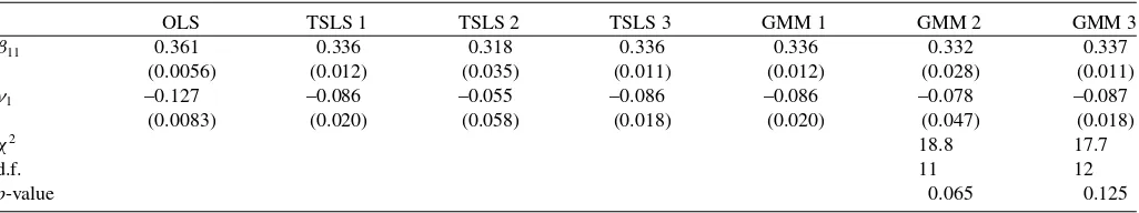
Table 1 summarizes the empirical results. Ordinary least squares, which does not account for mismeasurement, has an estimated log total expenditure coefficient ofγ1 = −0.127. Or-dinary two-stage least squares, using log total income as an instrument, substantially reduces the estimated coefficient to
γ1= −0.086. This is model TSLS 1 or equivalently GMM 1 in Table 1. TSLS1 and GMM 1 are exactly identified and so are numerically equivalent.
If we did not observe income for use as an instrument, we might instead apply the GMM estimator based on Corollary 4, using the moments cov(Z, ε1ε2)=0. As discussed in the Introduction, with classical measurement error, we may letZ
equal all the elements of X except the constant. The result is model GMM 2 in Table 1, which yieldsγ1= −0.078. This is relatively close to the estimate based on the external instru-ment log income, as would be expected if income is a valid instrument and if this article’s methodology for identification and estimation without external instruments is also valid. The standard errors in GMM 2 are a good bit higher than those of GMM 1, suggesting that not having an external instrument hurts efficiency.
The estimates based on Corollary 4 are overidentified, so the GMM 2 estimates differ numerically from the two-stage least squares version of this estimator, reported as TSLS 2, which uses (Z−Z)ε2 as instruments (Equation (14)). The GMM 2 estimates are closer than TSLS 2 to the income-instrument-based estimates GMM 1 and have smaller standard errors, which shows that the increased asymptotic efficiency of GMM is valu-able here. A Hansen (1982) test fails to reject the overidentifying moments in this model at the 5% level, though thep-value of 6.5% is close to rejecting.
Table 1 also reports estimates obtained using both mo-ments based on the external instrument, log income, and on cov(Z, ε1ε2)=0. The results in TSLS 3 and GMM 3 are very similar to TSLS 1 and GMM 1, which just use the external instrument. This is consistent with validity of both sets of iden-tifying moments, but with the outside instrument being much stronger or more informative, as expected. The Hansen test also fails to reject this joint set of overidentifying moments, with a
p-value of 12.5%.
To keep the analysis simple, possible mismeasurement of the food budget share arising from mismeasurement of total expenditures, as in Lewbel (1996), has been ignored. This is not an uncommon assumption, for example, Hausman, Newey, and Powell (1995) is a prominent example of Engel curve estimation assuming that budget shares are not mismeasured and log total expenditures suffer classical measurement error (though with the complication of a polynomial functional form). However, as a check, the Engel curves were reestimated in the form of quantities of food regressed on levels of total expenditures. The
results were more favorable than those reported in Table 1. In particular, the ordinary least squares estimate of the coefficient of total expenditures was 0.124, the two-stage least squares estimate using income as an instrument was 0.172, and the two-stage least squares estimate using this article’s moments was 0.174, nearly identical to the estimate based on the outside instrument.
One may question the validity of the assumptions for apply-ing Theorem 1 in this application. Also, although income is commonly used as an outside instrument for total expenditures, it could still have flaws as an instrument (e.g., it is possible for reported consumption and income to have common sources of measurement errors). In particular, the estimates show a re-versal of the usual attenuation direction of measurement error bias, which suggests some violation of the assumptions of the classical measurement error model, for example, it is possible that the measurement error could be negatively correlated with instruments or with other covariates.
Still, it is encouraging that this article’s methodology for ob-taining estimates without external instruments yields estimates that are close to (though not as statistically significant as) esti-mates that are obtained by using an ordinary external instrument, and the resulting overidentifying moments are not statistically rejected.
In practice, this article’s estimators will be most useful for applications where external instruments are either weak or un-available. The reason for applying it here in the Engel curve context, where a strong external instrument exists, is to verify that the method works in real data, in the sense that this article’s estimator, applied without using the external instrument, pro-duces estimates that are very close to those that were obtained when using the outside instrument. The fact that the method is seen to work in this context where the results can be checked should be encouraging for other applications where alternative strong instruments are not available.
5. SET IDENTIFICATION-RELAXING IDENTIFYING ASSUMPTIONS
This article’s methodology is based on three assumptions— namely, regressorsXuncorrelated with errorsε, heteroscedas-tic errorsε, and cov(Z, ε1ε2)=0. As shown earlier, this last assumption arises from classical measurement error and omit-ted factor models, but one may still question whether it holds exactly in practice. Theorem 3 shows that one can still identify sets, specifically interval bounds, for the model parameters when this assumption is violated by assuming this covariance is small rather than zero. Small here means that this covariance is small relative to the heteroscedasticity inε2; specifically, Theorem 3
assumes that the correlation betweenZ andε1ε2 is smaller (in
magnitude) than the correlation betweenZandε2 2.
For convenience, Theorem 3 is stated using a scalarZ, but given a vectorZ, one could exploit the fact that Theorem 3 would then hold for any linear combination of the elements of
Z, and one could choose the linear combination that minimizes the estimated size of the identified set.
DefineWj by Equation (11) for j =1,2. Given a random
scalarZand a scalar constantζ defineŴ1as the set of all values ofγ1that lie in the closed interval bounded by the two roots (if
Table 1. Engel Curve Estimates
OLS TSLS 1 TSLS 2 TSLS 3 GMM 1 GMM 2 GMM 3 β11 0.361 0.336 0.318 0.336 0.336 0.332 0.337
(0.0056) (0.012) (0.035) (0.011) (0.012) (0.028) (0.011) γ1 –0.127 –0.086 –0.055 –0.086 –0.086 –0.078 –0.087
(0.0083) (0.020) (0.058) (0.018) (0.020) (0.047) (0.018)
χ2 18.8 17.7
d.f. 11 12
p-value 0.065 0.125
NOTES: OLS is an ordinary least squares regression of food shareY1on household characteristicsXand log total expendituresY2. TSLS 1 is this regression estimated using two-stage least squares with log real income as an ordinary external instrument. TSLS 2 is this article’s heteroscedasticity-based estimator, Equation (14), which uses (Z−Z)ε2as instruments, whereZis all the regressorsXexcept the constant. TSLS 3 uses both (Z−Z)ε2and the outside variable log real income as instruments. GMM 1, GMM 2, and GMM 3 are the same three models estimated by efficient GMM, based on Corollary 4.
Reported above areβ11=X′β, which is the Engel curve intercept at the mean of theXregressors, andγ1, which is the Engel curve slope coefficient ofY2. Standard errors are in parentheses. Also reported is the Hansen (1982) specification test chi-squared statistic for the overidentified GMM models 2 and 3, along with its degrees of freedom andp-value.
they are real) of the quadratic equation:
[cov (W1W2, Z)]2
covW2 2, Z
2 −
var (W1W2) varW2
2
τ2+2
covW1W2, W22
varW2 2
τ2
− cov (W1W2, Z)
covW22, Z
γ1+1−τ2γ12=0. (15)
Also, define B1 as the set of all values of β1=
E(XX′)−1E[X(Y
1−Y2γ1)] for eachγ1∈Ŵ1.
Theorem 3. Let Assumption A1 hold for the model of Equa-tions (6) and (7). Assume E(Xε1)=0, E(Xε2)=0, and for
some observed random scalarZand some nonnegative constant
τ <1,|corr(Z, ε1ε2)| ≤τ|corr(Z, ε2
2)|. Then the structural
pa-rametersγ10 andβ10 are set identified byγ10∈Ŵ1,β10∈B1, andβ20is point identified byβ20=E(XX′)−1E(XY2).
Note that an implication of Theorem 3 is that Equation (15) has real roots whenever|corr(Z, ε1ε2)|<|corr(Z, ε2
2)|, andτis
defined as an upper bound on the ratio of these two correlations. The smaller the value ofτ is, the smaller will be the identified setsŴ1andB1, and hence the tighter will be the bounds onγ10
andβ10 given by Theorem 3. One can readily verify that the
setsŴ1andB1collapse to points, corresponding to Theorem 1,
whenτ =0.
An obvious way to construct estimates based on Theorem 3 is to substituteWj =Yj −X′E(XX′)−1E(XYj) into Equation
(15), replace all the expectations in the result with sample aver-ages, and then solve for the two roots of the resulting quadratic equation givenτ. These roots will then be consistent estimates of the boundary of the interval that bracketsγ10.
To illustrate the size of the bounds implied by Theorem 3, consider the model:
Y1=β11+Xβ12+Y2γ1+ε1, ε1=U+eXS1 (16)
Y2=β21+Xβ22+ε2, ε2 =U+e−XS2, (17) whereX,U,S1, andS2are independent standard normal scalars,
Z=X, andβ11=β12 =β21=β22=γ1=1. A supplemental
appendix to this article includes a Monte Carlo analysis of the estimator using this design. It can be shown by tedious but straightforward algebra that for this design, Equation (15)
re-duces to:
1−12+12e
2 −e4
+3e8
2+4e2−e4+3e8 τ 2
+2
5+7e2 −e4
+3e8
2+4e2−e4+3e8τ 2
−1
γ10
+1−τ2γ102 =0. (18)
Evaluating these equations for various values ofτshows that the identified regionŴ1forγ10is quite narrow unlessτis very close to its upper bound of 1. In this design, the true value isγ10=1, which equals the identified region whenτ =0.Forτ =0.1,the identified interval based on Equation (18) is [0.995,1.005], and for τ =0.5,the identified interval is [0.973,1.023]. Even for the loose bound on cov(Z, ε1ε2) given byτ =0.9, the identified interval is still the rather narrow range [0.892,1.084].
6. NONLINEAR MODEL EXTENSIONS
This section considers extending the model to allow for non-linear functions ofX. Details regarding regularity conditions and limiting distributions for associated estimators are not provided, because they are immediate applications of existing estimators once the required identifying moments are established.
6.1 Semiparametric Identification
Consider the model
Y1 =g1(X)+Y2γ10+ε1 (19)
Y2 =g2(X)+Y1γ20+ε2, (20)
where the functions gj(X) are unknown. In this simultaneous
system, each equation is partly linear as in Robinson (1988).
Assumption B1. Y =(Y1, Y2)′, whereY1andY2 are random variables. For some random vectorX, the functionsE(Y |X) andE(Y Y′|X) are finite and identified from data.
Given a sample of observations ofY andX, the conditional expectations in Assumption B1 could be estimated by nonpara-metric regressions, and so would be identified. These conditional expectations are the reduced form of the underlying structural model.
Assumption B2. E(ε1|X)=0,E(ε2 |X)=0, and for some random vectorZ, cov(Z, ε1ε2)=0.
As before, the elements ofZcan all be elements ofXalso, so no outside instruments are required. No exclusion assumptions are imposed, so all of the same regressorsXthat appear ing1
can also appear ing2, and vice versa. Ifεj =U αj+Vj, where
U,V1, andV2 are mutually uncorrelated (conditioning onZ), cov(Z, ε1ε2)=0 ifZis uncorrelated withU2.
Assumption B3. DefineWj =Yj −E(Yj |X) for j =1,2.
The matrixW, defined as the matrix with columns given by
the vectors cov(Z, W12) and cov(Z, W22), has rank 2.
Assumption B3 is analogous to Assumption A3, but employs a different definition ofWj. These definitions will coincide if
the conditional expectation ofYgivenXis linear inX. Lemma 1 continues to hold with this new definition ofWj and hence
of W, and more generally heteroscedasticity of W1 andW2
implies heteroscedasticity ofε.
Theorem 4. Let Equations (19) and (20) hold. If Assumptions B1 and B2 hold, cov(Z, ε22)=0, andγ20 =0,then the structural parameterγ10, the functionsg1(X) andg2(X), and the variance of εare identified. If Assumptions B1, B2, B3, and A4 hold, then the structural parametersγ10andγ20, the functionsg1(X) andg2(X), and the variance ofεare identified.
An immediate corollary of Theorem 4 is that the partly linear simultaneous system
Y1 =h1(X1)+X2β10+Y2γ10+ε1 (21)
Y2 =h2(X1)+X2β20+Y1γ20+ε2, (22)
where X=(X1, X2) will also be identified, since gj(X)=
hj(X1)+X2βj0is identified.
6.2 Nonlinear Model Estimation
Consider the model
Y1 =G1(X, β0)+Y2γ10+ε1 (23)
Y2 =G2(X, β0)+Y1γ20+ε2, (24)
where the functions Gj(X, β0) are known and the parameter
vector β0, which could include γ1 andγ2, is unknown. This
generalizes Equations (3) and (4) by allowing nonlinear func-tions of X. Letting gj(X)=Gj(X, β0), Theorem 4 provides
sufficient conditions for identification of this model, assum-ing that β0 is identified given identification of the functions
gj(X)=Gj(X, β0). The immediate analog to Corollary 3 is
then thatβ0,γ10,γ20, andµ0can be estimated from the moment conditions:
E[(Y1−G1(X, β0)−Y2γ10)|X]=0
E[(Y2−G2(X, β0)−Y1γ20)|X]=0
E(Z−µ0)=0
E[(Z−µ0) [Y1−G1(X, β0)−Y2γ10]
×[Y2−G2(X, β0)−Y1γ20]=0.
For efficient estimation in this case, where some of the mo-ments are conditional, see, for example, Chamberlain (1987), Newey (1993), and Kitamura, Tripathi, and Ahn (2003). Ordi-nary GMM can be used for estimation by replacing the first two
conditional moments above with unconditional moments:
E[ζ(X)(Y1−G1(X, β0)−Y2γ10)]=0
E[ζ(X)(Y2−G2(X, β0)−Y1γ20)]=0.
For some chosen vector valued functionζ(X), asymptotic ef-ficiency may be obtained by using an estimated optimalζ(X); see, for example, Newey (1993) for details.
As in the linear model, some of these moments may be weak, which would suggest the use of weak instrument limiting distri-butions in the GMM estimation. See Stock, Wright, and Yogo (2002) for a survey of applicable weak moment procedures.
6.3 Semiparametric Estimation
Consider estimation of the partly linear system of Equations (19) and (20), where the functionsgj(X) are not parameterized.
We now have identification based on the moments:
E[Y1−g1(X)−Y2γ10 |X]=0
E[Y2−g2(X)−Y1γ20 |X]=0
E(Z−µ0)=0
E[(Z−µ0) (Y1−g1(X)−Y2γ10)
×(Y2−g2(X1)−Y1γ20)]=0.
These are conditional moments containing unknown parame-ters and unknown functions and so general estimators for these types of models may be applied. Examples include Ai and Chen (2003), Otsu (2003), and Newey and Powell (2003).
Alternatively, the following estimation procedure could be used, analogous to the numerically simple estimator for linear
simultaneous models described earlier. Assume we haven
in-dependent, identically distributed observations. LetHj(X) be a
uniformly consistent estimator ofHj(X)=E(Yj |X), for
ex-ample, a kernel or local polynomial nonparametric regression of
YjonX. Now, as defined by Assumption B3,Wj =Yj −Hj(X),
so letWj i=Yj i−Hj(Xi) for each observationi. Next, letCj kh
be the sample covariance ofWjWkwithZh, whereZhis theh′th
element of the vectorZ. AssumeZ has a total ofKelements. Based on Equation (27), estimateγ1andγ2by
(γ1,γ2)=arg min (γ1,γ2)∈Ŵ
K h=1
(1+γ1γ2)C12h−γ1C22h−γ2C11h
2 ,
whereŴis a compact set satisfying Assumption A4. The above estimator forγ1andγ2is numerically equivalent to an ordinary nonlinear least squares regression overKobservations of data, where K is the number of elements ofZ. In a triangular sys-tem, that is, withγ2=0, this step reduces to a linear regression
for estimatingγ1. Finally, estimates of the functionsg1(X) and g2(X) are obtained by nonparametrically regressingY1−Y2γ1
andY2−Y1γ2 onX, respectively. The consistency of this pro-cedure follows from the consistency of each step, which in turn is based on the steps of the identification proof of Theorem 4.
This estimator ofγ1andγ2is an example of a semiparamet-ric estimator with nonparametsemiparamet-ric plug-ins (see, e.g., section 8 of Newey and McFadden 1994). Unlike Ai and Chen (2003), this numerically simple procedure might not yield efficient esti-mates ofγ1andγ2. However, assuming thatγ1andγ2converge
at a faster rate than nonparametric regressions, the limiting dis-tributions of the estimates of the functions g1(X) and g2(X)
will be the same as for ordinary nonparametric regressions of
Y1−Y2γ10andY2−Y1γ20onX, respectively.
Further extension to estimation of the partly linear system of Equations (21) and (22) is immediate. For this model, the
which could again be consistently estimated by the above de-scribed procedure, replacing the nonparametric regression steps with partly linear nonparametric regression estimators, such as Robinson (1988), or by directly applying an estimator, such as Ai and Chen (2003), to these moments.
7. CONCLUSIONS
This article describes a new method of obtaining identification in mismeasured regressor models, triangular systems, simulta-neous equation systems, and some partly linear semiparametric systems. The identification comes from observing a vector of variablesZ (which can equal or be a subset of the vector of model regressorsX) that are uncorrelated with the covariance of heteroscedastic errors. The existence of such aZ is shown to be a feature of many models in which error correlations are due to an unobserved common factor, including mismeasured regressor models. Associated two-stage least squares and GMM estimators are provided.
The proposed estimators appear to work well in both a small Monte Carlo study (provided as a supplemental appendix to this article) and in an empirical application. Citing working paper versions of the present article, some articles by other researchers listed earlier include empirical applications of the proposed estimators and find them to work well in practice.
Unlike ordinary instruments, identification is obtained even when all the elements ofZare also regressors in every model equation. However,Zshares many of the convenient features of instruments in ordinary two-stage least squares models. As with ordinary instrument selection, given a set of possible choices for
Z, the estimators remain consistent if only a subset of the avail-able choices are used, so variavail-ables that one is unsure about can be safely excluded from theZvector, with the only loss being efficiency. Similarly, as with ordinary instruments, if some vari-ableZsatisfies the conditions to be an element ofZ, but is only observed with classical measurement error, then this mismea-suredZcan still be used as an element ofZ. IfZhas more than two elements (or more than one element in a triangular system), then the model parameters are overidentified and standard tests of overidentifying restrictions, such as Hansen’s (1982) test, can be applied.
The identification here is based on higher moments and so is likely to give noisier, less reliable estimates than identification
based on standard exclusion restrictions, but may be useful in applications where traditional instruments are weak or nonexis-tent. This article’s moments based on cov(Z, ε1ε2)=0 can be
used along with traditional instruments to increase efficiency and provide testable overidentifying restrictions.
This article also shows that bounds on estimated pa-rameters can be obtained when the identifying assumption cov(Z, ε1ε2)=0 does not hold, provided that this covariance is not too large relative to the heteroscedasticity in the errors. In a numerical example, these bounds appear to be quite narrow.
The identification scheme in the article requires the endoge-nous regressors to appear additively in the model. A good direc-tion for future research would be searching for ways to extend the identification method to allow for including the endogenous regressors nonlinearly. Perhaps it would be possible to replace linearity in endogenous regressors with local linearity, apply-ing this article’s methods and assumptions to a kernel weighted locally linear representation of the model.
It would also be worth considering whether additional mo-ments for identification could be obtained by allowing for more general dependence betweenZandε2
2 and corresponding zero
higher moments. One simple example is to let the assumptions of Theorems 1 and 2 hold using̟(Z) in place ofZfor different functions̟, such as higher moments ofZ, thereby providing additional instruments for estimation.
ACKNOWLEDGMENTS
I thank Roberto Rigobon, Frank Vella, Todd Prono, Su-sanne Schennach, Jerry Hausman, Raffaella Giacomini, Tiemen Woutersen, Christina Gathmann, Jim Heckman, and anonymous referees for helpful comments. Any errors are my own.
APPENDIX
Proof of Theorem 1. Define Wj by Equation (11) for
j =1,2. These Wj are identified by construction. Using
the Assumptions, substituting Equations (6) and (7) for
Y1 and Y2 in the definitions of W1 and W2 shows that
W1=ε1+ε2γ10 and W2=ε2, so cov(Z, ε1ε2)=0 is
equiv-alent to cov[Z,(W1−γ10W2)W2]=0. Solving forγ10 shows
that γ10 is identified by γ10=cov(Z, W1W2)/cov(Z, W22).
Given identification of γ10, the coefficients β10 and β20 are identified by β10=E(XX′)−1E[X(Y1
−Y2γ10)] and β20= E(XX′)−1E(XY2), which follow from E(Xε
j)=0. Also, ε
is identified byε1=Y1−X′β10−Y2γ10andε2=Y2−X′β20.
Finally, to show Equation (8), observe thatZXsimplifies to:
ZX=
which spans the same column space as
E(XX′) 0
E(ZXε2) cov(Z, ε22)
,
and so has rank equal to the number of columns, which makes
ZXZXnonsingular. Also
E
which then gives Equation (8).
Proof of Theorem 2. Substituting Equations (9) and (10) for
Y1andY2in the definitions ofW1andW2shows that:
W1=
ε1+ε2γ10
1−γ10γ20, W2=
ε2+ε1γ20
1−γ10γ20, (A.1)
and solving these equations forεyields:
ε1=W1−γ10W2, ε2=W2−γ20W1. (A.2)
Note thatγ10γ20=1 by Assumption A4. Using Equation (A.3),
the condition cov(Z, ε1ε2)=0 is equivalent to:
cov[Z,(W1−γ10W2)(W2−γ20W1)]=0
(1+γ10γ20)cov(Z, W1W2)−γ10cov(Z, W22)
−γ20cov(Z, W12)=0. (A.3)
Now 1+γ10γ20=0, since otherwise, it would follow from
Equation (A.3) that the rank ofW is less than 2. Define
λ1= γ10
1+γ10γ20, λ2 = γ20
1+γ10γ20 (A.4)
andλ=(λ1, λ2)′, then we have:
cov(Z, W1W2)=λ1covZ, W22+λ2covZ, W12=Wλ,
(A.5)
soλis identified by:
λ=(′WW)−1′Wcov(Z, W1W2),
and′
WWis not singular becauseWis rank 2. Solving
Equa-tion (28) forγ10gives:
0=λ2γ102 −γ10+λ1.
The above quadratic inγ10 has at most two roots, and for each root, the corresponding value forγ20is given byγ20=γ10λ2/λ1. Let (γ1∗,γ2∗) denote one of these solutions. It can be seen from
λ1=
1
γ10 +γ20 −1
, λ2=
1
γ20 +γ10 −1
that the other solution must be (γ2∗−1,γ1∗−1), since that yields the same values forλ1 andλ2. One of these solutions must be
(γ10,γ20), and by Assumption A4, the other solution is not an element ofŴ, so (γ10,γ20) is identified. Note that the conditions required for the quadratic to have real rather than complex or imaginary roots are automatically satisfied, because (γ10,γ20) is real.
Given identification ofγ10andγ20, the coefficientsβ10andβ20
are identified byβ10=E(XX′)−1E[X(Y1−Y2γ10)] andβ20= E(XX′)−1E[X(Y2−Y1γ20)], which follow fromE(Xεj)=0.
Finally, ε is now identified by ε1=Y1−X′β10−Y2γ10 and
ε2=Y2−X′β20−Y1γ20.
Proof of Lemma 1. Equation (A.1) in Theorem 2 was derived
using only Assumptions A1 and A2. Evaluating cov(Z, W2
j)
using Equation (A.1) and the assumption that cov(Z, ε1ε2)=0
gives, for each elementZkofZ
cov(Zk, W12)
cov(Zk, W22)
=
1 1−γ10γ20
2
1 γ102 γ2
20 1
cov(Zk, ε12)
cov(Zk, ε22)
,
(A.6)
soWis rank 2 if and only ifεis rank 2 and the matrix relating
the two above is nonsingular, which requires|γ10γ20| =1.
Proof of Corollary 1. Using Equation (A.2) and following the same steps as the proof of Theorem 2, the conditionE(Zε1ε2)=
0 yields
E(ZW1W2)=λ1EZW22+λ2EZW12=Wλ
instead of Equation (A.5). This identifiesλand the rest of the proof is the same.
Proof of Corollary 2. β20andγ20, and henceε2, are identified
from the usual moments that permit two-stage last squares esti-mation. EachWj is identified as in Theorem 1, and by Equation
(A.1), cov(Z, ε1ε2)=0 implies cov[Z,(W1−γ10W2)ε2]=0, which when solved forγ10gives
γ10=cov(Z, W1ε2)/cov(Z, W2ε2)
and cov(Z, W2ε2)=cov(Z, ε22)=0, so γ10 is identified. The rest of the proof is the same as the end of the proof of Theorem 2.
Proof of Corollaries 3 and 4. By Equations (9) and (10),
Q1 =Xε1,Q2=Xε2andQ4=(Z−µ)ε1ε2, andE(Q3)=0
makesµ=E(Z), soE(Q)=0 is equivalent to E(Xε1)=0, E(Xε2)=0, and cov(Z, ε1ε2)=0. It then follows from
Theo-rem 2, or from TheoTheo-rem 1 whenγ20=0, that the onlyθ∈
that satisfiesE[Q(θ, S)]=0 isθ=θ0.
Proof of Theorem 3. First observe that if cov(Z, ε22)=0, then this fact along with the other assumptions would imply that the conditions of Theorem 1 hold, giving point identification, which is a special case of the statement of Theorem 3. So, for the re-mainder of the proof, assume the case in which cov(Z, ε22)=0. Note this means also thatvar(ε22)=0 andvar(Z)=0, because
var(ε22)=0 orvar(Z)=0 would imply cov(Z, ε22)=0. These inequalities will ensure that the denominators in the fractions given below are nonzero.
By the definition ofτ:
corr (ε1ε2, Z)/corrW22, Z2 ≤τ2
[cov (ε1ε2, Z)]2
var (ε1ε2) var (Z)
varW22var (Z)
covW2 2, Z
2 ≤τ 2
[cov (ε1ε2, Z)]2
covW22, Z2 ≤
var (ε1ε2) varW22τ
2 .