www.elsevier.com/locate/spa
Measurements of ordinary and stochastic
dierential equations
Jan Ub
H
e
Department of Engineering, Stord=Haugesund College, BjHrnsonsgate 45, 5528 Haugesund, Norway
Received 15 March 1999; received in revised form 29 February 2000; accepted 29 February 2000
Abstract
Solutions to stochastic dierential equations depends on the method of approximation. In this paper we give a very simple demonstration that ordinary dierential equations, too, exhibit this kind of behavior when the coecients are measure-valued distributions. We then proceed to show that the Itˆo and the Stratonovich solutions can be viewed as similar cases within this framework. c2000 Elsevier Science B.V. All rights reserved.
MSC:60H10; 34A10; 46F10
Keywords:Ordinary and stochastic dierential equations; Multiplication of generalized functions
1. Introduction
The measurement method was introduced in LindstrHm et al. (1995). The basic
mechanism is to smoothen distributions by an approximate identity and to study limits of such expressions. Of course, this is nothing but a variation over a classical theme in functional analysis and as such not very original. The approach originates from ideas related to the theory of Colombeau distributions, see Colombeau (1990). In this theory,
generalized functions F are identied by mappings 7→F(x), where x7→F(x) are
smooth functions.
Functional objects of the above kind have found many applications. In particular, they have been used extensively to study properties of stochastic partial dierential equations, see, e.g., Colombeau et al. (1996), Holden et al. (1993), Holden et al. (1994), Oberguggenberger (1992), and Oberguggenberger and Russo (1997). The ap-proach in this paper, however, takes a slightly dierent direction. Here we want to study the connection between ordinary and stochastic dierential equations. Our pur-pose is to show that the non-uniqueness of solutions to stochastic dierential equations,
i.e., Itˆo=Stratonovich solutions, corresponds to a similar kind of non-uniqueness that we
nd in ordinary dierential equations with measure-valued coecients.
While the basic theory of Colombeau distributions is very important to justify that products of generalized functions are uniquely dened, the measurement method
provides a simplied approach to search for solutions to (generalized) dierential
equa-tions. To study a (generalized) dierential equation on the form Lu= 0, we are only
concerned with the limiting behavior of smoothed versions of the left-hand side. If this can be shown to be arbitrary small, we say that we have a solution. In principle, the left-hand side can involve several products of generalized functions. Our approach is then to view the left-hand side as a joint object, and we make no eort to justify the denition of each individual term.
The paper is organized as follows. In Section 2 we formulate the basic concepts in the measurement method. We prove that if all the coecients in a dierential equation
areC∞, then a distribution is a solution in the measurement sense if and only if it is a
solution in the classical sense of distributions. In Section 3 we consider the dierential
equation F′+·F= 0 whereis a (non-random) measure, and can easily demonstrate
that dierent solution concepts for this equation gives a multitude of dierent solutions.
In Section 4 we study the more complex case where is a white noise measure. We
prove that the Itˆo and the Stratonovich solutions can be viewed as two dierent cases within this framework. Thus the non-uniqueness of solutions to stochastic dierential equations can be viewed as a special case of the non-uniqueness of ordinary dierential equations with measure valued coecients.
2. The measurement method
Let D be a domain in Rd, let D denote the space of test functions on D, i.e., the
set of all∈Cc∞(D) with the usual test function topology, and let D′ denote the dual
space of distributions. For each multi-index = (1; 2; : : : ; d), we let D denote the
dierential operator
D=
@ @x1
1
· · ·
@ @xd
d
: (2.1)
Although the method below can be extended to cover non-linear operators, we will in this paper always consider the linear case, i.e., we consider a formal dierential
operator L on the form
Lu= X ||6N
f·Du: (2.2)
We will assume that u∈D′ and also that all f∈D′. Note that the productsf·Du
do not necessarily make sense as distributions, so we will need to make a more rened denition.
The interpretation goes like this; choose and x 0∈Cc∞(Rd) with the properties
0¿0 and
R
Rd0(x) dx= 1. Then consider the family n(x) :=nd0(nx); n∈N. This
we will call a family of measurements, and 0 is called the core of the measurement.
In general, we may want to perform dierent measurements on the dierent terms
in (2.2). To this end, we will for each multi-index consider two families of
formal expression (2.2), we now associate what we call an error function
En(u)(x) = X
||6N
(f∗;1; n(x))(Du∗;2; n(x)); (2.3)
where the ∗ denotes a convolution product. We now want to consider dierential
equations which formally can be written in the form
Lu= 0: (2.4)
If is some xed topology, we say that u∈D′ is a 0-measurement solution to (2.4)
in the -topology if
lim
n→∞En(u) = 0 in the-topology: (2.5)
When all the coecients f ∈C∞(Rd), then (2.4) also makes sense in the space of
distributions. In this case, however, we have the theorem below.
Theorem 2.1. Choose and x any cores for the measurements. If all f ∈C∞(Rd);
D=Rd; and is the topology of convergence in the sense of distributions; then the following statements are equivalent:
(A) u solves Lu= 0 in the sense of distributions.
(B) u is a 0-measurement solution to Lu= 0 in the -topology.
Proof. Choose and x any multi-index . Since each f is smooth, f∗;1; n→f
in C∞(Rd) with its usual Frechet space topology. Clearly every Du
∗;2; n →Du
in D′. Using Theorem 6:18 in Rudin (1980), we get
lim
n→∞En(u) =Lu (2.6)
and the theorem follows trivially from this.
If the coecients f are not smooth, however, the measurement solutions are more
exible than classical solutions in the sense of distributions. Note that with the denition
above, we are not required to make sense to the product of the distributions fu.
If only we can prove thatEn(u)→0 in some appropriate topology, we have a solution.
Initial conditions: Since we want to consider distribution solutions to dierential
equations, we need to consider this in relation with initial values. IfF is a continuous
function, we certainly have
F(0) = lim
n→∞F(n): (2.7)
This we use as a denition for the general case, i.e., we say that a distribution F has
a point value F0 at 0 if
lim
n→∞F(n) =F0: (2.8)
3. Equations with singular coecients
Let t0¿0 and consider the initial value problem
F′+t0F= 0; F(0) =F0 (3.1)
on [0;∞). Here t0 denotes the Dirac delta function at t0. This problem can be
ad-dressed in several dierent ways. One way of approach is to smooth the singular
coecient t0, and consider the limit of such expressions. More precisely, we put
F= limn→∞Fn where each Fn is the solution to
Fn′+ (t0∗n)Fn= 0; Fn(0) =F0: (3.2)
It is then trivial to see that
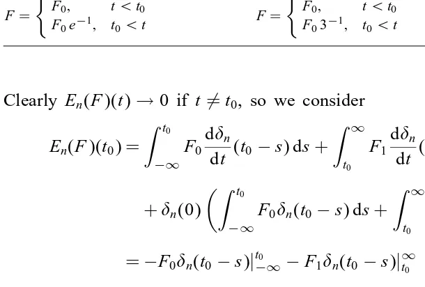
F=
(
F0; 06t ¡ t0;
F0e−1; t0¡ t:
(3.3)
We remark that we only consider distributions here, so we can leave F undened at
t0. From the above point of view, only the coecient t0 is subject to measurement.
If F, too, is subject to a simultaneous measurement, we consider the error function
En(F)(t) =
dF
dt ∗n(t) + (t0∗n(t))(F∗n(t)): (3.4)
Here and in the remaining part of this section, we will always assume that all
mea-surements have a common core 0. The problem is now to nd a distribution F s.t.
En(F)(t)→0 in some appropriate topology. It is of some surprise to observe that this
approach does not reproduce solution (3.3). It actually turns out that the solution is
depending on certain characteristics of the core 0. We wish to prove the following
proposition.
Proposition 3.1. With the core 0 xed; the function
F=
F0; 06t ¡ t0;
F0
1 + (1=R0∞0(−u) du)
; t0¡ t
(3.5)
solves (3:1)in the 0-measurement sense with the topology of pointwise convergence.
Proof. For simplicity of notation we let F1= F0 1+(1=R∞
0 0(−u) du)
. Then we get
En(F)(t) = Z t0
−∞
F0
dn
dt (t−s) ds+
Z ∞
t0
F1
dn
dt (t−s) ds
+n(t−t0) Z t0
−∞
F0n(t−s) ds+ Z ∞
t0
F1n(t−s) ds
Table 1
Solutions to the initial value problem (3.1)
Smoothed coecients Symmetric cores Anticipating cores
F=
The solutions above will in general depend on 0. If 0 is a symmetric function,
however, we always get the same solution. In relation to stochastic dierential equations
we will also need to consider the case where 0 is supported on (−∞;0]. Such cores
we will call anticipating. For easy reference, we show the results in Table 1.
The question of uniqueness, too, is related to special properties of the core 0. To
examine this further, we consider a distribution supported att0. Using Theorem 6:25
in Rudin (1980), we know that
=
Unless the core 0 satises
we can nd 6= 0 s.t. En()(t)→0 for all t. So if (3.11) fails, then (3.1) has
innitely many solutions. With this in mind, we dene the indierence set, IDS,
of a core 0 by
IDS(0) :={k∈N:(0k)(0)0(0)−(0k+1)(0) = 0}: (3.12)
We can then characterize all the solutions to (3.1):
Proposition 3.2. If F is a0-measurement solution to (3:1)in the topology of
point-wise convergence; then
F= +
F0; 06t ¡ t0;
F0
1 + (1=R∞
0 0(−u) du)
; t0¡ t;
(3.13)
where =PN
k=0akDkt0 and all ak= 0 if k6∈IDS(0).
Proof. Let G be any distribution solving (3.1) in the 0-measurement sense. If K is
any compact set withk∩ {t0}=∅, then if n is large enought0∗n(t) = 0 for allt∈K.
Hence we must have G′= 0 on K. It follows that
G= +
G0; 06t ¡ t0;
G1; t0¡ t;
(3.14)
where is supported att0 and G0; G1 are constants. By the initial condition G0=F0.
Using the calculations preceding this proposition, we get
En(G)(t0) = N X
k=0
ak(−1)knk+2(0(k)(0)0(0)−(0k+1)(0))
+n0(0)
G1+ (G1−G0) Z ∞
0
0(−s) ds
: (3.15)
This converges to zero if and only if G1=F1 and allak= 0 when k∈IDS(0).
Corollary 3.3. IfIDS(0) =∅; then
F=
F0; 06t ¡ t0;
F0
1 + (1=R∞
0 0(−u) du)
; t0¡ t (3.16)
is the unique solution to (3:1)in the 0-measurement sense.
It is easy to nd cores where IDS(0) =∅. One example of such kind occurs when
0 is symmetric with (2k)(0)6= 0 for all k. In this case
F=
F0; 06t ¡ t0;
F03−1; t0¡ t
(3.17)
is the unique solution to (3.1) in the 0-measurement sense.
We will now proceed to a more general case. We want to consider the initial value problem
where is a measure. As we will see from the calculations below, not every measure admits solutions in the measurement sense. We will therefore need to equip the measure with some additional structure.
Put tp0 = 0, and let Sf={tif}i∞=1 and Sp={tip}∞i=1 be two strictly increasing
se-quences of positive real numbers. We dene two measuresf andp as follows; Let
f: [0;∞)→R be a piecewise continuous function with singularities in Sf, i.e.,
Sf=
x: lim
u→x− f(u)= lim6 u→x+f(u)
: (3.19)
Letf be the corresponding measure having f as its density w.r.t. Lebesgue measure.
Let p be a pure point measure with positive point masses concentrated inSp, i.e.
p=
∞
X
i=1
mitpi: (3.20)
In the rest of this section, we will restrict our attention to symmetric cores. If 0 is
symmetric with 0(0)6= 0, then IDS(0) has a particularly simple form. The following
easy lemma will be useful in the discussion below.
Lemma 3.4. Assume that 0 is a symmetric core with 0(0)6= 0; then
(a)
IDS(0) ={k:If k is even; then (0k)(0) = 0; if k is odd; then (k+1)
0 (0) = 0}:
(3.21)
(b) If m6= 0 is any real number; then k∈IDS(0)⇔m(0k)(0)0(0)−(0k+1)(0) = 0.
(c) If k∈IDS(0); then (0k)(0) = 0.
(d) IDS(0) =∅ ⇔0(2k)(0)6= 0 for all k∈N.
Proof. When0 is symmetric, then(0k)(0)=0 for all odd numbersk. Then (a) follows
trivially from (3.12), and (b), (c), and (d) are immediate consequences of (a).
Theorem 3.5. Let =f+p. Assume that Sf∩Sp=∅ and that 0 is a symmetric
core with IDS(0) =∅.Then
F=
Fie
−Rt tipf(s) ds
; tip¡ t ¡ tip+1;
i= 0;1; : : : ;
Fi+1e
−Rt tp i+1
f(s) ds
; tip+1¡ t ¡ tip+2 ;
(3.22)
where
Fi+1=Fi 2
−mi+1
2 +mi+1
e−
Rtip+1
tip f(r) dr
; i= 0;1; : : : (3.23)
is the unique solution to the initial value problem(3:18)in the0-measurement sense
Proof. For simplicity of notation we only consider the casei=0. Ift6∈Sp, then clearly
Now observe that since 0 is a symmetric core, then
Z ∞
Using (3.22), we integrate by parts to rewrite (3.21)
=
If is a distribution supported at t1p, then using essentially the same argument as
before, we get
since IDS(0) =∅. Uniqueness then follows from essentially the same calculation as in
Proposition 3.2.
Theorem 3.6. If 0 is a symmetric core with IDS(0) =6 ∅ and 0(0) 6= 0; then
all solutions to (3:18) in the 0-measurement sense with the topology of pointwise
convergence; can be written on the form
G=
Proof. For simplicity, we only consider the case where i= 1. Using (3.26) and (3.27) we get
we get
En(1+F)(t1p) = N−1 X
k=0
ak;1(−1)knk+2(m10(k)(0)0(0)−(0k+1)(0))
+ (f(t1p) + O(n))
N−1 X
k=0
ak;1(−1)knk+1(0k)(0) + O(n): (3.31)
Theorem 3.6 then follows by repeated use of this argument.
As is also clear from the proof of Theorem 3.5, the solution always fails if f has
a discontinuity at some tpi+1. To get a solution in this case, F1 must satisfy the two
equations
F1−F0e
−Rt p i+1
tpi f(r) dr+mi 2
F1+F0e
−Rt p i+1
tpi f(r) dr
= 0;
F1−F0e
−Rt p i+1
tp i
f(r) dr
(f(t p
i+1−)−f(t p
i+1+)) = 0:
(3.32)
System (3.32) has no solution unlessmi=0. Hence it will not be possible to extend the
result in Theorem 3.5 to arbitrary measures on R+. This, however, does not exclude
the possibility that other types of measures can be considered. In the next section we
will consider the case where is a white noise measure.
4. Stochastic dierential equations
LetBt(!) be a Brownian motion on a probability space (; P;F). We will not need
any special structure on , so we do not specify this further. Ft=(Bs;s6t) is the
ltration generated by the Brownian motion Bt. For ∈D we consider the mapping
W(; !) =R
(s) dBs. Since the mapping 7→ W() is well dened, almost linear
and continuous in probability onD, it has a version W ∈D′, see Walsh (1986). Note
that W is independent of what version we use for the stochastic integrals. Since the
integrands are non-random, smooth functions, we get exactly the same mapping using both the Itˆo and the Stratonovich interpretation of the stochastic integral.
Again we want to consider the initial value problem
F′+F= 0; F(0) =F0; (4.1)
this time with the random measure=+W; ; ∈R. Formally this version of (4.1)
corresponds to the linear stochastic dierential equation
dFt=−Ftdt−FtdBt: (4.2)
It is well known that if we consider the limit of a sequence
Fn′+ (∗n)Fn= 0; Fn(0) =F0; (4.3)
then the sequence Fn converges to the Stratonovich solution of (4.2). In the literature
of Wong and Zakai (1969). Since then this paradox has been extended in several dierent directions by a large group of researchers. See Twardowska (1996) for a considerable list of references to previous work within the eld. Just to mention a few we here refer to, e.g., Sussmann (1978), Protter (1985), and Kurtz and Protter (1991). In particular, Protter (1985) extends the Wong–Zakai approach to equations with path-dependent coecients driven by arbitrary semi-martingales. In a quite recent paper Twardowska (1996), the author gives an extensive survey on approximation result related to the Wong–Zakai approach and similar approximation schemes for stochastic dierential equations.
The basic topic for the above-mentioned papers, however, is that one considers limits of solutions of a sequence of equations approaching a limiting equation. From this point of view, the approach in the present paper is basically dierent. Here the dierential equation is xed, and we use limits to examine whether or not a given candidate is a solution to the equation.
A similar kind of method can be found with reference to Wick multiplication, ♦,
within the context of white noise analysis, see, e.g., Hida et al. (1993), Holden et al. (1996). The equation
F′+ (a+bWt)♦F= 0 (4.4)
can be solved using a Wick power series expansion in Bt, and the solution coincides
with the Itˆo solution to (4.2) Hu andIksendal (1996), consider approximation schemes
similar to the Wong–Zakai approach for certain quasilinear stochastic dierential equa-tions formulated in terms of Wick products. They conjecture that these approximaequa-tions might converge to the Itˆo solution, but give no proof of this.
As we have seen in Section 3, the measurement method often oers a dierent inter-pretation than the basic approach underlying the Wong–Zakai paradox. It is interesting to note that with a carefully selected collection of cores, the Itˆo solution of (4.2) is a solution to (4.1) in the measurement sense.
One cannot expect that the Itˆo solution solves (4.1) for any collection of cores. The choice of cores must somehow reect the underlying structure in the Itˆo integral. The construction goes like this:
We call a core 0 anticipating if it is supported at (−∞;0], and non-anticipating if
it is supported at [0;∞). We let ˆ0(x) =0(−x). So if 0 is anticipating, then ˆ0 is
non-anticipating and vice versa. The error function we want to consider is as follows:
En(F)(t; !) =
dF
dt ∗ˆn(t) + (∗ˆn(t))(F∗n(t)): (4.5)
As will be clear from the proof below, this collection of cores is essentially the only choice for which the theorem below holds true.
Theorem 4.1. If =+W; ; ∈R; 0 is a non-anticipating core; and the error
function is specied through (4:5); then the geometric Brownian motion
F(t; !) =F0e−(+
1 2
2)t−B
t (4.6)
Remark. Note that the Itˆo calculus plays no part in the formulation of the above result. In the proof of the statement, however, we will make extensive use of this calculus.
In what follows, integrals of the form R
(s; !) dBs are always interpreted in the Itˆo
sense.
Proof. Choose and x t ¿0 and let n be so large that all the cores are supported in (−nt; nt). Note that all the integrals below are really integrals with compact support; this will be important for some of the estimates below.
We want to discuss the cores at a general level to demonstrate why the special error function in (4.4) is needed. To this end, we start measuring the terms using three
dierent cores1; n; 2; n and3; n. ClearlyF(t; !) is the Itˆo solution of (4.2). Using this
together with the integration by parts formula for Itˆo integrals, we get
We rst consider the term Gn(!) =R
Taking the square inside integrals in the previous expression, we have used that 1;0
and 3;0 have compact support.
Now consider Hn(s; !) =R
∞
0 (F(r)2; n(t−s)−F(s)1; n(t−r))3; n(t−s) dr which
is the dicult case.
We want to prove that Hn(s; !) satises the following properties:
(a) E[R∞
0 |Hn(s; !)|ds]→0 as n→ ∞
(b) E[R0∞ |Hn(s; !)|2ds]6C whereC is some constant not depending on n.
We rst split Hn into several parts to be considered separately:
Hn(s; !) =
It suces to prove that (a) and (b) holds for each term I, II and III separately. We start with an estimate of II. The estimation for I is similar, and in fact simpler. Case III, however, is quite awkward and will need special attention. In the proofs
Proof of (a):
This proves (a). To prove (b), consider
E
This proves (b) in the case of term II. We now consider term
III =F(s)(2; n(t−s)−1; n(t−s)): (4.14)
Here there is no integration to scale down the term. In fact, unless this term is vanish-ing, there is little hope to prove any kind of estimates on III. In the theorem, we have
chosen 1=2= ˆ. Then III = 0, and thus Hn(s; !) satises (a) and (b). To proceed
further, we need to use the Itˆo isometry to control the size of R∞
cannot be done unless Hn(s; !) is adapted. Essentially, the only way to achieve this is
to let2; n and3; nhave disjoint support with2(t−s) supported ons¿t and3(t−r)
supported on r6t. In our theorem we have chosen 3=. Then the adaptedness
is OK.
To complete the proof of the theorem, we need to prove the following lemma.
Lemma 4.2. If a sequence of adapted processes Hn(s; !) satises
(a) E[R∞
0 |Hn(s; !)|ds]→0 as n→ ∞;
(b) E[R∞
0 |Hn(s; !)|
2ds]6C where C is some constant not depending on n,
then for any T ¿0 the sequence n =R0T Hn(s; !) dBs converges to zero in the
weak∗-topology onL2(P).
Proof. Pick any Y ∈L2(P). We need to prove that
E[nY]→0: (4.15)
Since
E[nY] =E[E[nY|FT]] =E[nE[Y|FT]]; (4.16)
we can assume, without loss of generality, that Y is FT-measurable. Then by the Itˆo
representation theorem, see Iksendal (1995), we can nd a predictable y(s; !) s.t.
Y =RT
0 y(s; !) dBs. By Itˆo’s formula, we then get
E[nY] =E Z T
0
Hn(s; !) dBs Z T
0
y(s; !) dBs
=E
Z T
0
Hn(s; !)y(s; !) ds
:
(4.17)
Since the unit ball in L2(×[0; T];dP× ds) is compact in the weak∗-topology, it
follows from (a) and (b) thatHn(s; !)→0 weakly in this space. Hence we have that
E[RT
0 Hn(s; !)y(s; !) ds]→0, and this completes the proof of the lemma.
Note that the adaptedness requirements on 0;ˆ0 implies that Hn are adapted. If we
then use the results from (4.11) and (4.13) together with Lemma 4.2, this completes the proof of Theorem 4.1.
We now turn to the question of uniqueness of the solution. To this end we consider a new process
G(t) =F0e
′
t+′
Bt; (4.18)
where′ and ′ are arbitrary constants. If we repeat the calculation in (4.7), we get
En(G)(t) = Z ∞
0
G(s)(3; n(t−s)−1; n(t−s)) ds
+
Z ∞
0 Z ∞
0
+
+′+1 2(
′)2 Z ∞
0
G(s)1; n(t−s) ds
+ (+′)
Z ∞
0
G(s)1; n(t−s) dBs: (4.19)
By exactly the same estimates as in the proof of Theorem 4.1, we see that the rst two terms goes to zero. For the third term we get
+′+1 2(
′)2 Z ∞
0
G(s)1; n(t−s) ds→
+′+1 2(
′)2
G(t): (4.20)
Unless +′= 0, the last term clearly explodes. Hence E
n(G)(t)→0 if and only if
′=− and′=−(+122). We summarize these results in the following proposition.
Proposition 4.3. Let G denote the class of processes on the form
Xt=F0e
′
t+′
Bt; ′; ′∈R: (4.21)
The Itˆo solution to (4:2)is the unique solution within G;to the initial value problem
(4:1) in the sense of the 0-measurements in (4:5).
Remark. From Proposition 4.3 we see that the Stratonovich solution is nota solution
in the sense of 0-measurements. In fact, from (4.19) it follows that the Stratonovich
solution is a solution in the 0-measurement sense to the modied equation
F′+ (−122+W)F= 0: (4.22)
Which, of course, also follows from the classical theory since the Stratonovich solution to (4.2) is known to coincide with the Itˆo solution to
dFt=−(−122)Ftdt−FtdBt: (4.23)
From Proposition 4.3, it seems likely to conjecture that the Itˆo solution is unique within
a much larger class than G. Preferably one should try to prove a result of this kind
dened within a class of generalized stochastic processes. Processes of this kind have been subject to intensive study for a number of years, in particular within the tradition of white noise analysis, see, e.g., Arnold (1974), Hida et al. (1993), Holden et al. (1996), and the references therein.
While the Itˆo solution seems to be the “right” solution with respect to the particular error function in (4.5), it would be interesting if one could choose a dierent set of cores such that the Stratonovich solution would satisfy (4.1) in the sense of measure-ments. This, however, seems quite hard to prove. The only option seems to be the
introduction of some overlap in the support of 2;0 and3;0. It is not clear if and how
one could manage to control the size of this term.
By comparison, the solution from smoothed coecients in (3.3) could also be
ob-tained from a carefully choosen core 0 in Proposition 3.1. This particular choice of
Table 2
Solutions to the initial value problem (4.2)
Limit of equations where the Solution in the sense of coecients are smoothed 0-measurements in (4.5)
Stratonovich solution Itˆo solution
We summarize the discussion in this section in Table 2. This table is to be compared with Table 1 in Section 3.
Acknowledgements
The author gratefully acknowledges several useful suggestions from the referees.
References
Arnold, L., 1974. Stochastic Dierential Equations: Theory and Applications. Wiley, New York. Colombeau, J.F., 1990. Multiplication of distributions. Bull. Am. Math. Soc. 23, 251–268.
Colombeau, J.F., Heibig, A., Oberguggenberger, M., 1996. Generalized solutions to partial dierential equations of evolution type. Acta Appl. Math. 45 (2), 115–142.
Hida, T., Kuo, H.-H., Pottho, J., Streit, L., 1993. White Noise Analysis. Kluwer, Dordrecht.
Holden, H., LindstrHm, T.,Iksendal, B., UbHe, J., Zhang, T.-S., 1993. Stochastic boundary value problems. A white noise functional approach. Probab. Theory Related Fields 95, 391–419.
Holden, H., LindstrHm, T.,Iksendal, B., UbHe, J., Zhang, T.-S., 1994. The Burgers equation with a noisy force and the stochastic heat equation. Comm. Partial Dierential Equations 19, 119–141.
Holden, H.,Iksendal, B., UbHe, J., Zhang, T.-S., 1996. Stochastic partial dierential equations — a modeling. White Noise Functional Approach. Birkhauser, Boston.
Hu, Y., Iksendal, B., 1996. Wick approximation of quasilinear stochastic dierential equations. In: Korezlioglu, H., Iksendal, B., Ustunel, A.S. (Eds.), Stochastic Analysis and Related Topics, Vol. 5. Birkhauser, Basel, pp. 203–231.
Kurtz, T.G., Protter, P., 1991. Weak limit theorems for stochastic integrals and stochastic dierential equations. Ann. Probab. 19 (3), 1035–1070.
LindstrHm, T.,Iksendal, B., UbHe, J., Zhang, T.-S., 1995. Stability properties of stochastic partial dierential equations. Stochastic Anal. Appl. 13 (2), 177–204.
Oberguggenberger, M., 1992. Multiplication of distributions and applications to partial dierential equations. Longman Scientic and Technical. Wiley, New York.
Oberguggenberger, M., Russo, F., 1997. Colombeau solutions and pathwise limits. In: Decreusefond, L., Gjerde, J., Ustunel, A.S.,Iksendal, B. (Eds.), Stochastic Analysis and Related Topics. Birkhauser, Basel, pp. 325–340.
Iksendal, B., 1995. Stochastic Dierential Equations, 4th Edition. Springer, Berlin.
Protter, P., 1985. Approximations of solutions of stochastic dierential equations driven by semi-martingales. Ann. Probab. 13 (3), 716–743.
Rudin, W., 1980. Functional Analysis. Springer, Berlin.
Sussmann, H.J., 1978. On the gap between deterministic and stochastic ordinary dierential equations. Ann. Probab. 60, 19–41.
Twardowska, K., 1996. Wong-Zakai approximations for stochastic dierential equations. Acta Appl. Math. 43 (3), 317–359.
Walsh, J.B., 1986. An introduction to stochastic partial dierential equations. In: Carmona, R., Kesten, H., Walsh, J.B. (Eds.), Ecole d’ Ete de Probabiletes de Saint-Flour XIV-1984. Springer, Berlin, pp. 265–437. Wong, E., Zakai, M., 1969. Riemann–Stieltjes approximations of stochastic integrals. Z. Wahr. Verw. Geb.