www.elsevier.com/locate/orms
Optimal control of a simple manufacturing system
with restarting costs
Y. Salama
∗Departement de Mathematiques, Ecole Polytechnique Federale de Lausanne, CH-1015 Lausanne, Switzerland
Received 1 July 1997; received in revised form 1 July 1999
Abstract
We consider the optimal control of an unreliable manufacturing system with restarting costs. In 1986 and 1988, Akella and Kumar (for the innite horizon discounted cost) and Bielecki and Kumar (for the innite horizon average expected cost) show that the optimal policy is given by an optimal inventory level (“hedging point policy”). Inspired by these simple systems, we explore a new class of models in which the restarting costs are explicitly taken into account. The class of models discussed often allow complete analytical discussions. In particular, the optimal policy exhibits an (s;S) type form. c2000 Elsevier Science B.V. All rights reserved.
Keywords:Optimal feedback control; HBJ equation; Bang–bang (s;S) policy; Restarting cost
1. Introduction
In this paper, we consider the problem of control-ling the production rate of a simple manufacturing system. Akella and Kumar [1] obtained the optimal policy for a single failure prone machine for an in-nite horizon discounted cost criterion. They show that the optimal policy depends on an optimal inven-tory levelz∗(“hedging point”). Under this policy the production rate is chosen to be maximum when the stock levelX(t) is belowz∗, zero whenX(t)¿ z∗and
equal to the demand rate whenX(t) =z∗. Bielecki and
Kumar [2] obtained a similar optimal policy which minimizes the long term average expected cost. In
∗Fax: +41-21-693-4303.
E-mail address:[email protected] (Y. Salama)
both of these models the cost functiong(x) depends only on the stock level, and is dened by
g(x) =C+x++C−x−; (1) wherex+= max(x;0) andx−= max(−x;0).
In this paper we will restrict the production rate of the machine, which is the controllable variable, to be dichotomous{0; M}, i.e. the machine can only pro-duce at a maximum speed or can be put in a stand-by state where it is not producing. We then introduce a restarting cost to be paid each time we decide to switch from the stand-by state to the producing one. We will show that adding this restarting cost leads to a “bang–bang” (s;S) type optimal policy. The opti-mal policyu(x; ) is quite simple and the control de-pends only on the stock position x and on the state of the machine(t). In the producing state, it consists in continuing producing ifx ¡ band switching to the
stand-by state if not. The stand-by state remains se-lected as long asx ¿ a; as soon asx6a a cost is incurred and the production is switched on at the rate
M (we clearly haveb ¿ a).
This paper is structured as follows: in the following section, we will describe the dynamic of the model and in Sections 3 and 4 we give the optimal policies which respectively minimizes the average and the discounted cost in innite horizon for a perfect machine (without failures). In Sections 5 and 6 we take into account random failures and a random repair time and we give the optimal policy for the same costs as in Sections 3 and 4. Finally in Section 7, we show that the (s;S) policy is optimal.
The results obtain in Sections 3–5 are limiting case of the general situation presented in Section 6. More precisely the control which minimizes the average cost is the limit of the control which minimizes the dis-counted cost for a discount→0 [4]. Similarly, the deterministic models are obtained for small values of the indisponibility factor I ==, where −1 is the mean time to failure and −1 the mean time to re-pair. We nevertheless give the results of the simpler models for two main reasons: explicit expressions are only tractable for the deterministic models and in Sec-tions 5 and 6 the methods used for the discounted and the average cases are dierent. For the sake of clarity, in Sections 5 and 6, we will expose the method but we give only explicit results for particular values of the parameters. General analytic formulas can easily be computed with the help of a program like Maple but the expressions obtained are too large to be pre-sented. Moreover, the values of the parametersaand
b, which denes the optimal control, are at the end, given in terms of solutions of transcendent equations.
2. Description of the model
We consider a failure prone machine producing a single product. There is a constant demanddfor this product and we can choose, whenever the machine is operating, to produce at rateM or not to produce, here the production rate cannot take intermediate values. The machine is subject to failures and can be repaired. We will suppose that the time to failure and the time needed to repair a failure are independent, exponen-tially distributed random variables with parameters
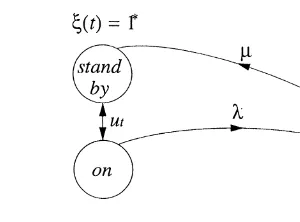
Fig. 1. Markov chain.
and. LetX(t) be the stock level of the product at time
t, given by the dierence between the cumulate pro-duction and the demand up to timet. Remark thatX(t) can be negative, i.e. we admit backlog.X(t) evolves as
dX(t)
dt =utM−d; (2)
whereut ∈ {0; I((t) 6= 0)} and where (t) is de-ned by the continuous-time Markov chain sketched in Fig. 1, and where
I((t)6= 0) =
0 if (t) is in o state at timet;
1 if not:
(3)
There are now three possible states, the on state: dX(t)=dt=M−d, the stand-by state: dX(t)=dt=−d
and the o state: dX(t)=dt=−d. The control variable
ut triggers the transition from the on to the stand-by state and conversely. We assume that the machine cannot fail while it is in the stand-by state. From now on we will, respectively, note “on” (or 1), “stand by” (1∗) and “o ” (0) for these states. The transitions on→o and o→stand by are governed by expo-nential distributions of parameters and. The pro-cess of interest is thus{X(t); (t)} whereX(t)∈ R and (t) ∈ {0;1;1∗}. The “deterministic cases” in
Sections 3 and 4 are given by the limit → 0 and
→ ∞.
The cost due to inventory is given byg(x)=C+x++
C−x−, where x+= max(x;0) andx−= max(−x;0).
minimizes
wherei are the times where we choose to go from the stand-by state ut = 0 to the on state ut = 1 and
Edenotes the expectation over the realizations of the stochastic process(t).
And for the average case:
J= lim
Remark that for the average case,J does not depend on the initial conditions any more.
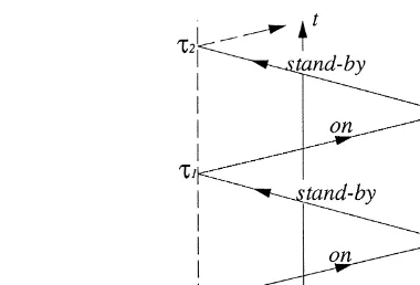
3. Deterministic system, average cost
As the machine cannot fail, we only have two states (on and stand-by) and the problem is deterministic. The dynamic is periodic and the control is given by two parametersaandb:
ut= control. The cost for one periodJ1 is given by
J1(a; b) =−C−
Fig. 2. Optimal control of the system.
−C−
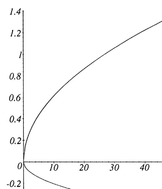
Fig. 3. Control as a function of the restarting costfor the values
M= 2; d= 1; C+= 20; C−= 60.
4. Deterministic system, discounted cost
For a deterministic discounted system, the cost de-pends on the initial conditions, but the control does not. Indeed we can nd the two parametersaandbby minimizing the expected discounted cost for the initial conditionX(t−0) = 0 and the machine in the produc-ing state. We start by calculatproduc-ing the cost J1(0;on) incurred during one cycle:
and we sum over all cycles taking into account the elapsed time:
aandbare slightly more complicated:
a=d
!1; (15)
where!1 is the solution of
(M −d) ln
where!2 is the solution of
(M −d) ln
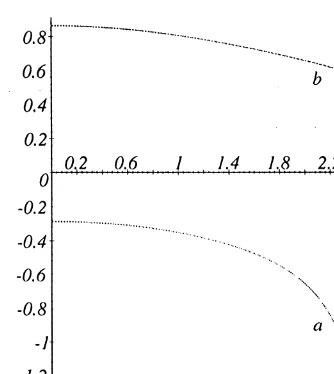
Fig. 4. Control as a function of the discount for the values
= 20; M= 2; d= 1; C+= 20; C−= 60.
havea=(d=) ln(z1) andb=[(M−d)=] ln(z2) where
z1andz2 are, respectively, the positive solutions of
z21+L
2+K2−(MC+)2
KL z1+ 1 = 0 (21)
and
z22+L
2−K2−(MC+)2
KMC+ z2+ 1 = 0: (22)
As expected, in the limit → 0 we nd again the values ofaandb(Eqs. (9) and (10)) for the average case. We show in Fig. 4 the values ofa andb as a function of the discount rate.
5. Stochastic system, average cost
For this case, we will proceed in two steps. First, we will nd the stationary distribution and then we will calculate its associate cost. The minimization over the parametersa andb will give us the optimal control law.
5.1. Stationary distribution
Let us denote by P0a(x) dx; P1a(x) dx and
P1∗a(x) dxthe probabilities of nding the stock level
in [x; x+ dx], respectively, in the state o, on and stand-by for x ¡ a. We denote the same probabili-ties for the region a ¡ x ¡ b by P0b(x); P1b(x) and
P1∗b(x). The stationary measure of the stochastic
process {X(t); (t)} subject to the previous control obeys, for the zone x6a, a balance equation of the form [3]:
d@
@xP0a(x) =− P1a(x) +P0a(x); (23)
(M −d) @
@xP1a(x) =− P1a(x) +P0a(x); (24)
P1∗a(x) = 0: (25)
Similarly for the zonea ¡ x6b;we have
d@
@xP0b(x) =− P1b(x) +P0b(x); (26)
(M −d) @
@xP1b(x) =− P1b(x); (27)
d@
@xP1∗b(x) =−P0b(x): (28)
These equations are linear partial dierential equation of the rst order, it is the easy to calculate their solu-tions. In order to x the integration constants, we then need to use the boundary conditions Eqs. (29) – (33) and the normalization Eq. (34). If, in the mean, we can satisfy the demand, we have
P1a(−∞) = 0: (29)
Whenx=b, we transit from the on state to the stand-by state:
P1∗b(b)d=P1b(b)(M −d): (30)
It is not possible to be at position x=b with the machine down:
P0b(b) = 0: (31)
The probability of being atx=awith the machine in the on state is the sum of the probability of coming from x ¡ a and the probability of coming from the right in the stand-by state:
P1b(a)(M−d) =P1∗b(a)d+P1a(a)(M −d): (32)
The probability of being in the o state is continuous ata:
Fig. 5. Stationary distribution for the valuesd=1; M=1:9; =12; =14; = 20; C+= 20; C−= 60.
Z a
−∞
(P1a(x) +P0a(x)) dx
+
Z b
a
(P1b(x) +P1∗b(x) +P0b(x)) dx= 1: (34)
Using Maple or a similar program, we easily nd analytically all the integration constants.
5.2. Cost associated to the stationary distribution
Here we have to distinguish the casea ¿0 from the casea60, we will only show the equations fora ¿0. The cost associated with the limit distribution is the sum of the cost due to the stock population plus the restarting cost ataand the restarting cost forx ¡ a:
J=
Z 0
−∞
−C−x(P1a(x) +P0a(x)) dx
+
Z a
0
C+x(P1a(x) +P0a(x)) dx
+
Z b
a
C+x(P1b(x) +P0b(x) +P1∗b(x)) dx
+P1∗b(a) +
Z a
−∞
P0a(x)dx: (35)
The optimal control is again given by minimizing the costJ overaandb. This minimization leads to cum-bersome expressions. We only give here the result
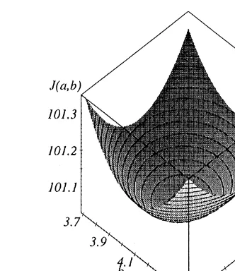
Fig. 6. Cost as a function ofaandbfor the valuesd= 1; M= 2;
=12; =14; = 20; C+= 20; C−= 60:
for the special valuesd= 1; M = 2; =1 2; =
1 4;
= 20; C+= 20; C−= 60. We nda= 1:71, and
b=4:06 for a “hedging point”, which would have been (if= 0)z∗= 3:9. We can verify that for the value
= 2 and=101, the result of the deterministic prob-lem is approached. In this case, we nda=−0:263 andb= 0:911, while in the deterministic case we have
a=−0:288 andb= 0:866. We show in Fig. 5 the sta-tionary distribution of the process (withM = 1:9 →
a= 2:55; b= 4:85 to avoid superposition of the curves) and in Fig. 6 the cost as a function ofaandb.
6. Stochastic system, discounted cost
We modify the problem assuming that the transition (control) from state 1 to 1∗ (respectively, from 1∗ to 1) is no more instantaneous, but that when we decide to transit we have a probabilitydt(respectively,dt) to transit in a time dt≪1 (exponential distribution). We also modify the restarting costand we now as-sume that we have a costper unit time when we try to transit from the stand-by (1∗) state to the on (1)
state.
by J1(x); J1∗(x) and J0(x). The Hamilton–Bellman–
Jacobi equations for this problem are
0 =g(x)−d@J0(x)
Now, we will suppose the control known, which will divide the space into four regions (again we have to distinguish the casea ¿0 from the casea60). Here we will treat the case a ¡0: region A is dened by
x ¡ a, region B by a6x ¡0, region C by 06x ¡ b
and region D byb6x. We obtain for each of the re-gions, a system of partial dierential equations, for example in the C region
@
where we have put a subscript c to indicate that x
is in the region C. We solve these equations in each region of the space and we stick together the costs corresponding to the dierent regions:
Jai(a) =Jbi(a); Jbi(0) =Jci(0); Jci(b) =Jdi(b) (42)
fori= 1;1∗and 0. With these equations, we can nd
the integration constants and we nd the minimum of
Jb0(0) for example, with respect toaandb. Note here that, as the policy is optimal, the minimization of any,
J::(x) at any pointxleads to the same values ofaand
b.
For the case = 101; d = 1; M = 2; = 12; =14; = 20; C+= 20; C−= 60, we nda=−0:107 and b= 1:553, which agree exactly with numerical results (dynamic programming).
7. Optimality of the (s;S) policy
In this section, we will show that the (s;S) policy is optimal. Only the case of the stochastic system with a discounted cost will be considered as the others are limiting cases.
Up to now, we have only found the optimal val-ues of a and b for a (s;S) policy and we have to show that these solutions give the minimum of the expected discounted cost over all acceptable policies. Unfortunately, the algebra seems to become too heavy to allow a direct proof in the general case. To cir-cumvent this diculty, we can compute the expected discounted cost for any given values of the parame-ters and then show that it does indeed satisfy the HBJ equations (36) – (38). To illustrate this procedure, we treat explicitly the case discussed in Section 6 and we show that the (s;S) policy is optimal in this case.
By construction, the costsJ1(x); J1∗(x) andJ0(x) are
solutions of the Eqs. (36) – (38) for a specic choice ofu. Therefore, we only have to check that the minima in these equations are obtained for our choice ofu. Eqs. (37) and (38) can be rewritten as
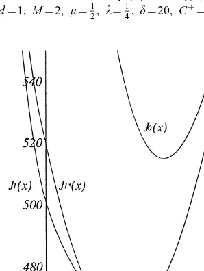
Fig. 7. Dierence between J1∗(x) and J1(x) for the values
=101; d=1; M=2; =12; =14; =20; C+=20 andC−=60.
Fig. 8. Optimal costs J1(x); J1∗(x) and J0(x) for the values
=101; d=1; M=2; =12; =14; =20; C+=20 andC−=60:
(s;S) control asJ1(x) =J1∗(x)− in region A and
J1(x) =J1∗(x) in region D. Between a andb where
the policy does not switch from one state to the other, we have to show that
J1(x)6J1∗(x)6J1(x) +: (47)
Fig. 7 shows that, whenaandbare optimal, condition (47) is satised. In Fig. 8, we sketch the optimal costs
J1(x); J1∗(x) andJ0(x).
Acknowledgements
The author is grateful to M.-O. Hongler and E. Boukas for stimulating discussions and remarks.
References
[1] R. Akella, P.R. Kumar, Optimal control of production rate in a failure prone manufacturing system, IEEE Trans. Automat. Control AC-31 (1986) 116–126.
[2] T. Bielecki, P.R. Kumar, Optimal of zero-inventory policies for unreliable manufacturing system, Oper. Res. 36 (1988) 532–541.
[3] W. Feller, An Introduction to Probability Theory and its Applications, Vols. 1 and 2, Wiley, New York, 1971. [4] P.R. Kumar, P. Varaiya, Stochastic Systems: Estimation,