TERRASAR-X INSAR PROCESSING IN NORTHERN BOHEMIAN COAL BASIN USING
CORNER REFLECTORS (PRELIMINARY RESULTS)
Ivana Hlav´aˇcov´a, Lena Halounov´a, Kvˇetoslava Svobodov´a
Department of Mapping and Cartography, Remote Sensing Laboratory Faculty of Civil Engineering
Czech Technical University Th´akurova 7, 166 21 Prague 6, Czech republic
[email protected], [email protected], [email protected] Commission VII/2
KEY WORDS:SAR interferometry, artificial corner reflectors, phase unwrapping, decorrelation, manual processing
ABSTRACT:
The area of Northern Bohemian coal basin is rich in brown coal. Part of it is undermined, but large areas were mined using open-pit mines. There are numerous reclaimed waste dumps here, with a horse racetrack, roads and in some cases also houses. However, on most of the waste dumps, there are forests, meadows and fields. Above the coal basin, there are the Ore mountains which are suspected to be sliding down to the open mines below them.
We installed 11 corner reflectors in the area and monitor them using the TerraSAR-X satellite. One of the reflectors is situated in the area of radar layover, therefore it cannot be processed. We present preliminary results of monitoring the remaining corner reflectors, with the use of 7 TerraSAR-X scenes acquired between June and December 2011.
We process whole scene crops, as well as the artificial reflector information alone. Our scene set contains interferometric pairs with perpendicular baselines reaching from 0 to 150 m. Such a configuration allows us to distinguish deformations from DEM errors, which are usual when the SRTM (Shuttle Radar Topography Mission) DEM (X-band) is used for Stripmap data.
Unfortunately, most of the area of interest is decorrelated due to vegetation that covers both the Ore mountains and the reclaimed waste dumps. We had to enlarge the scene crop in order to be able to distinguish deformations from the atmospheric delay. We are still not certain about the stability of some regions.
For the installed artificial reflectors, the expected deformations are in the order of mm/year. Generally, deformations in the area of interest may reach up to about 5 cm/year for the Ervˇenice corridor (a road and railway built on a waste dump).
When processing artificial corner reflector information alone, we check triangular sums and perform the processing for all possible point combinations — and that allows us to correct for some unwrapping errors. However, the problem is highly ambiguous.
1 INTRODUCTION
The history of brown-coal mining in the Northern-Bohemian coal basin is very long. Since the 15thcentury, people have tried var-ious ways of mining the coal — and the area is full of old “wild” mines, deep mines (usually from the beginning of the 20th cen-tury), and since about 1950s, there are huge open-pit mines with large waste dumps. In the region, stable areas are very small, with lava on top of the coal making mining very difficult; such places are built-up to form villages, towns, industrial zones etc. Some villages, known to be built on coal, are now being considered to be demolished.
Above the coal basin, there are the Ore mountains, which are sus-pected to be sliding down into the basin. In order to monitor this slide, 11 artificial reflectors were installed in the area. The reflec-tors were oriented in order to be monitored by the TerraSAR-X satellite (Stripmap mode with resolution of about 3x3 meters) in the descending pass, and regularly cleaned (a day before the pass because the passes are performed early in the morning). Five of the corner reflectors are situated in various built-up areas in the region, one is situated almost in the center of the open mine (on a rock), two are just below the Ore mountains and two are in the slope of the Ore mountains (however, one of them cannot be seen due to the radar artefacts). The distance between the reflectors is about 3–5 km, their configuration can be found in figure 2. The expected deformations are low for the reflectors, in the order
of millimeters per year, and therefore the acquisitions are per-formed usually once per 33 days.
2 CONVENTIONAL INTERFEROMETRIC
PROCESSING
Using the 7 acquired scenes (see table 1), 21 interferograms were formed (each with each other). For DEM subtraction, SRTM (Shuttle Radar Topography Mission) (Farr et al., n.d.) X-band DEM was used. The TerraSAR-X data are also in the X-band, and also the resolution is better (1 arc sec, i.e. approx 30 m) in comparison to classical SRTM (C-band) DEM. In comparison to ASTER DEM (with the same resolution), the results are much smoother. Unfortunately, the SRTM X-band DEM does not have 100% coverage for our latitude (about 50o), and that is why part of the scene crop could not be processed.
However, the SRTM DEM was acquired in 2000, and since that time, the open mines changed significantly. Therefore the inter-ferometric phase in the area of open mines changes very quickly in space (if coherent). On the other hand, these phase variations are caused by DEM errors, and such areas cannot be used for atmospheric delay estimation. In addition, the DEM must be strongly interpolated in order to correspond to the resolution of the scenes.
06–07 06–08 06–09 06–10 06–11 06–12 07–08
07–09 07–10 07–11 07–12 08–09 08–10 08–11
08–12 09–10 09–11 09–12 10–11 10–12 11–12
Figure 1: All processed interferograms. 06 stays for the scene acquired on June 17, 2011, 07 for the scene acquired on July 20, 2011, 08 for the scene acquired on August 22, 2011, 09 for the scene acquired on September 24, 2011, 10 for the scene acquired on October 27, 2011, 11 for the scene acquired on November 29, 2011, and 12 for the scene acquired on December 21, 2011.
date BT[days] B⊥[m] weather
17-06-2011 0 0 unknown
20-07-2011 33 -145 heavy rain 22-8-2011 66 3 clear sky, very hot 24-9-2011 99 -143 dry (possible or fog)
27-10-2011 132 -12 fog
29-11-2011 165 -84 probably fog 21-12-2011 187 -12 thin layer of snow Table 1: Data used, together with temporal and perpendicular baselines. The data were acquired by the TerraSAR-X satellite in the StripMap mode (with incidence angle 29–32 degrees. Mas-ter scene is in bold and the temporal and perpendicular baselines refer to it.
the scene acquired in December are all much more decorrelated, which is caused by the fact that at that time, there was a thin layer of snow on the ground.
3 INSAR PROCESSING OF THE ARTIFICIAL REFLECTOR INFORMATION ONLY
In comparison to conventional interferometric processing, the phase of the installed artificial reflector is expected to be much more precise. This is due to the fact that the reflectors are designed to reflect a high amount of the received radar energy back to the antenna, and therefore the reflector should be the major scatterer in a pixel.
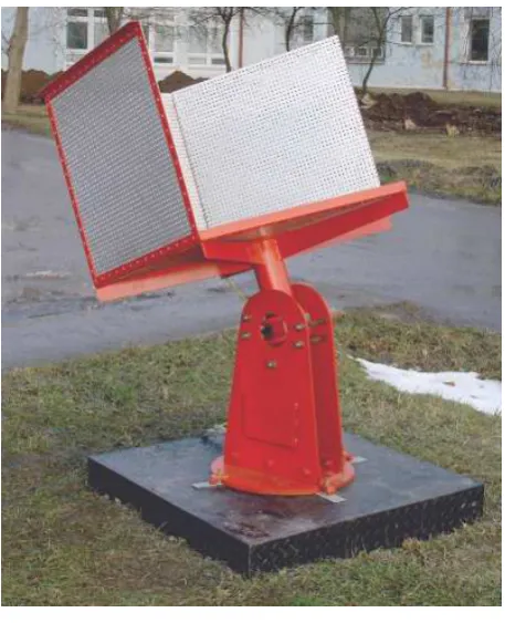
In fact, the reflectors are not exactly “corner reflectors”. By a mis-understanding, the bottom plane is a pentagon, with three planes perpendicular to it. Therefore, its properties should be close to a dihedral reflector (Ferretti et al., 2007). All edges of the pen-tagon are approx. 70 cm long, and so is the height of the three square planes. It is constructed from punched metal plate. Re-flector orientation can be adjusted in both the azimuth and the zenith direction. The reflector is fixed to a block of concrete. A picture of a reflector can be found in figure 3.
The configuration of artificial reflectors in the radar image can be found in figure 2.
All artificial reflectors (except for one, which is probably situated in radar layover) were found in the scenes as approximately 2x2
Figure 2: A map of the artificial reflectors in the scene crop (smaller than in figure 1) Corner reflector no. 9 is not visible in the radar image due to its position in the radar layover. Original data cDLR.
very light pixels (intensity of about106 –107
), and can be there-fore well recognized from their surroundings. According to the intensity, the coordinates were estimated with the sub-pixel preci-sion (in the GAMMA software (GAMMA, n.d.)), and the phase was also interpolated. However, these interpolated results were not used yet, and will be used in future — to do that, the flat-Earth phase and the topographic phase need to be recomputed for the interpolated coordinates.
DEM correction was performed for the pixels with the installed reflectors, on the basis of levelled heights. Correction of the height between the leveling point and the reflector edge was not performed, it is constant for all reflectors.
Figure 3: A photo of a reflector.
However, SAR interferometry only works between two dates and between two points (so-called double-difference). We therefore define that on June 17, 2011 (first acquisition), the deformations were zero. In addition, we pair our reflectors each with each other in order to perform spatial referencing. Below, we will see that it is neccessary in order to get consistent results.
3.1 Triangular sums
The phase of the interferograms is expected to fulfill the triangu-lar sum condition. Let us take three scenes, compute the three in-terferograms (each with each) and sum the interferogram phases (for one point). The phase sum is expected to be zero — if the in-terferograms are with or without flat-Earth phase, with or without topographic phase, spatially/temporally referenced or not. Due to noise, it is not exactly zero, but in our case it is usually smaller than 0.3–0.4 rad. It is slightly higher only for some interferogram triples. Such a measure can give us an idea about the precison of the phase — concerning primarily coregistration (resampling) errors. However, in this measure, many error sources are not in-cluded: thermal noise, atmospheric delay variation, DEM errors, orbit errors, deformations. On the other hand, triangular sums reach higher values for incoherent pixels.
If a triangular sum reaches a value near±2π, for the accuracy estimation it can be reduced by this value. Later, we will also use triangular sums as an indication of a “phase unwrapping error”. In our project, no phase unwrapping is performed. There are no fringes in the interferograms (see figure 1), only possible trends or quick color changes. In addition, the interferograms are decor-related to a high extent, and the coherent open-pit mines with lots of “false” fringes would bring many errors into the process. In the processing of the artificial reflector information alone, we will therefore estimate the phase ambiguities manually.
3.2 Deformation model
Deformation model according to (Usai, 2001) can be written as
ϕ=A·d=−4π
whereλis the radar wavelength,dare the deformations (in me-ters) together with atmospheric delay variations, orbit errors and other error influences with respect to an acquisition date. TheA matrix lacks one column (the first), i.e. it is already referenced to the first acquisition date. Theϕvector contains phase differences between two (reflector) points, for all interferograms.
First, theϕvectors for all pairs of points were reduced by inte-ger multiples of2πin order for the values to be in the(−π, π)
interval. Then, adjustment was performed and the adjustment standard deviations checked.
The value of the adjustment standard deviation isσ0 =qrTr np,
whererare the adjustment residues andnpis the number of mea-surements minus the number of unknowns. It indicates the num-ber of “unwrapping errors” for each reflector pair (see table 2). In some cases,σ0is close to 0 (0.1 rad at maximum): the residues are small. In some cases,σ0 is between 1.3 and 1.4: in these cases, one residue is about±4–5 rad and if corrected by 2π (with the appropriate sign),σ0 gets close to 0. Also, triangular sums indicate the one interferogram to be corrected.
In some cases, theσ0value is about 1.7 rad. In these cases, two interferograms are to be corrected by an integer multiple of2π. It can also be recognized (by the value ofσ0) if the two interfer-ograms have a common scene (lowerσ0) or not (σ0>1.8). If more interferograms have to be corrected by±2π, the situa-tion is more complicated: the residues are very similar, and the analysis of the triangular sums yields more “equivalent” solutions (different interferograms are to be corrected, but the number of them is the same, and so is the resultingσ0). The issue is that — considering that we have 7 scenes — if six interferograms (con-taining one certain scene) are corrected by the same multiple of
2π(taking into account if the scene is master or slave in each in-terferogram), the resultingσ0is the same, and so are the residues and triangular sums. Only the adjusted deformations differ: for the one scene, which was adjusted, they differ exactly by2π, i.e.
λ
2 ≈1.6cm in our case.
Such an adjustment was performed for all reflector pairs. There were 10 visible reflectors, i.e. 45 pairs. Out of those, 13 pairs gotσ0close to zero without any corrections, see table 2. For ad-ditional 6 pairs,σ0 can be lowered to a value close to zero by correcting one interferogram. Two corrections are neccessary for additional 7 reflector pairs. We did not try to correct the remain-ing reflector pairs with higherσ0because such corrections would be highly ambiguous.
However, comparing the results from various reflector pairs, we find out that the results are not consistent. If one tries to compute the deformations for a reflector pair which could not be computed directly (due to highσ0) and tries to compute it via another re-flector, different ways can give different values (by multiples of
2π).
refl. no 2 3 4 5 6 7 8 10 11 1 2.04 0.034 1.84 1.38 0.050 0.053 0.046 1.82 0.028 2 - 2.12 1.75 2.04 2.12 1.73 2.22 2.14 1.73 made, and forσ0≈1.7, two corrections were made. The remaining reflector pairs were not corrected.
First, we created six triangles (or quadrangles) from the pairs with no corrections. In such triangles, the sums of the adjusted defor-mations (between the two reflectors in the pair) are also expected to be zero. However, for some triangles, this is not the case — it is close to±2π. In these cases, one reflector pair must be selected and corrected by2πfor the scene with inconsistent results; i.e. 6 interferograms must be corrected (considering that the triangle gives±2πonly for one scene).
To ascertain the reflector pair to be corrected, we also made trian-gles and quadrantrian-gles using the pairs with one or two corrections. Here, the number of triangles with sums of±2πwas higher (in few cases there were±2πalso for more scenes). If all scenes give
±2πresults, it is sufficient to correct the2πambiguities only for the reference scene. In most cases, the corrections were simple (we correct one or two reflector pairs), but in one case, it was very difficult to analyze which pairs are to be corrected. Finally, the corrections were performed in these cases:
• June scene: reflector pair 2–11,
• July scene: reflector pairs 5–8, 10–11, 1–6, 6–8, 6–7, 6–10,
• August scene: reflector pair 2–7,
• December scene: reflector pairs 2–11, 8–11. 3.3 Velocity model
The velocity model, adapted from (Berardino et al., 2002), esti-mates only two unknowns: the (constant) deformation velocity and the height correction. Its disadvantage is that the deforma-tions are approximated by a linear model (together with other influences, such as atmospheric delay variations or orbit errors). On the other hand, the difference between the number of knowns and unknowns is higher here, and so it is easier to estimate the integer multiples of2πto be added to the measured phases. The velocity model, according to (Hlav´aˇcov´a, 2008), can be ex-pressed as
wheredtare the temporal baselines (for all interferograms),B⊥
are their perpendicular baselines,RM is the (approximate) dis-tance between the satellite and the point on the surface, andΘis the look angle. The unknowns arev(deformation velocity) and
∆h(height correction).
For the processing using the velocity model, we used the reflec-tor pair phases corrected by2πmultiples, as described in the de-formation model. We processed all pairs of reflectors with zero triangular sums, i.e. those that were corrected or where no cor-rection was neccessary.
4 RESULTS AND DISCUSSION
4.1 Deformation model
Values ofσ0 before 2π ambiguity corrections can be found in table 2. All reflector pairs with σ0 < 1.8 were corrected to σ0 < 0.1. The other pairs were not corrected at all and are excluded from further consideration. Figure 4 contains the es-timated deformations of all reflectors with regard to reflector 1. For those reflectors that have highσ0 with regard to reflector 1 (refl. no. 2, 4, 10), the estimated deformations were computed via other points (7 for refl. 2, 5 for refl. 4, 11 for refl. 10). Due to the overall consistency of the estimated deformations, which was tested using many (30–40) spatial triangular sums, the deforma-tions can be computed this way (spatial triangular sums are in the order of10−14
rad).
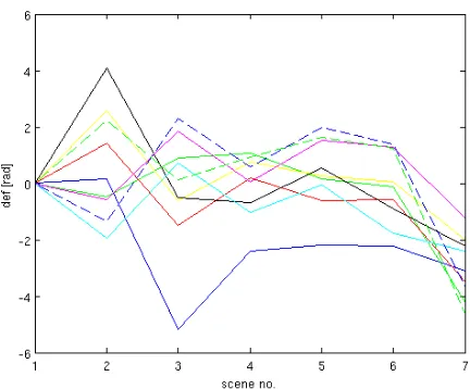
Analysing figure 4, there are two peaks, which are not probable: for reflector 2 (solid blue) it is the August scene, and for reflec-tor 6 (solid black) the July scene. Let us take into account that reflector pair 1–6 was corrected for the July scene, and reflector pair 2–7 was corrected for the August scene (reflector pair 1–2 was not processed, so it was computed as the sum of 1–7 and 7–2). In both cases, we can consider “shifting” (i.e. correcting) some other scenes by2πin order to get rid of the peak; however, in order to preserve consistency, the number of corrections by2π would be very high — for many interferograms and many other reflector pairs. And it is very probable that other peaks would emerge.
4.2 Velocity model
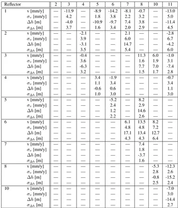
The results of the velocity model adjustment are displayed in ta-ble 3. There are both the deformation velocity and its standard deviation, together with the height correction with its standard deviation.
For topographic phase subtraction, we used levelled heights with accuracy in the order of centimeters. The height of the reflec-tor above the levelling mark was not considered because it is the same for all reflectors and therefore it is eliminated after spatial referencing. However, as noted in (Ketelaar, 2008), an inaccu-rately known (sub-pixel) range position has the same influence to the phase as the height error, so we attribute the height correc-tions to this fact, and also to the fact that the deformacorrec-tions are now approximated by a linear (in time) trend. Real separation of de-formation velocities and height errors will be achieved for more acquisitions, if the temporal and perpendicular baselines are not correlated (Kampes, 2006).
Reflector 2 3 4 5 6 7 8 10 11 1 v [mm/y] — -11.9 — -8.9 -14.2 -8.1 -0.7 — -13.0
σv[mm/y] — 4.2 — 1.8 3.8 2.2 3.2 — 5.0
∆h[m] — -4.0 — -10.9 -9.7 7.4 3.8 — -11.4 σ∆h[m] — 3.7 — 1.6 3.4 2.0 2.9 — 4.5
2 v [mm/y] — — -2.1 — — 2.1 — — -2.8
σv[mm/y] — — 3.9 — — 6.0 — — 6.7
∆h[m] — — -3.1 — — 14.7 — — -4.2
σ∆h[m] — — 3.5 — — 5.4 — — 6.0
3 v [mm/y] — — -0.4 — — — 11.3 6.0 -1.0
σv[mm/y] — — 3.6 — — — 1.6 1.9 3.1
∆h[m] — — -6.3 — — — 7.7 7.0 -7.4
σ∆h[m] — — 3.2 — — — 1.5 1.7 2.8
4 v [mm/y] — — — 3.4 -1.9 — — — -0.7
σv[mm/y] — — — 1.1 3.4 — — — 3.4
∆h[m] — — — -0.6 0.6 — — — 1.1
σ∆h[m] — — — 1.0 3.0 — — — 3.0
5 v [mm/y] — — — — -5.2 — 8.2 — —
σv[mm/y] — — — — 2.4 — 2.9 — —
∆h[m] — — — — 1.2 — 14.6 — —
σ∆h[m] — — — — 2.2 — 2.6 — —
6 v [mm/y] — — — — — 6.1 13.5 8.2 —
σv[mm/y] — — — — — 4.8 4.8 7.2 —
∆h[m] — — — — — 17.1 13.4 12.7 —
σ∆h[m] — — — — — 4.3 4.3 6.4 —
7 v [mm/y] — — — — — — 7.4 — —
σv[mm/y] — — — — — — 1.8 — —
∆h[m] — — — — — — -3.7 — —
σ∆h[m] — — — — — — 1.6 — —
8 v [mm/y] — — — — — — — -5.3 -12.3
σv[mm/y] — — — — — — — 2.8 2.6
∆h[m] — — — — — — — -0.8 -15.2
σ∆h[m] — — — — — — — 2.5 2.4
10 v [mm/y] — — — — — — — — -7.0
σv[mm/y] — — — — — — — — 3.0
∆h[m] — — — — — — — — -14.4
σ∆h[m] — — — — — — — — 2.7
Table 3: Deformation velocitiesvand their standard deviationsσv, together with height corrections∆hand their standard deviations σ∆h, computed for all reflector pairs with zero triangular sums (some of them were corrected using the deformation model).
be2πcorrected for more than two interferograms: see section 4.1.
Such unreliability cannot be easily solved now. The information about whether a reflector has moved or not is not known; and it is clear that we can manually correct any interferogram in any reflector pair. However, for the set to remain consistent, consid-ering triangular sums both for one (reflector) point, and spatial triangular sums between (reflector) points, there would have to be many corrections, and there is no measure about how close is a correction to the reality.
Considering the velocity model, the situation should get better with more scenes (to be acquired during 2012 with a period of 33 days), if there are more values of perpendicular baseline. How-ever, there is probably no possibility to estimate the atmospheric delay variation due to the huge decorrelation, so the atmosphere will still be contained in the adjusted results, only “smoothed”.
And finally, it is not known whether the deformations are really linear in time.
5 CONCLUSIONS AND FUTURE WORK
The problem of processing the reflector information alone is am-biguous to a high degree. Due to the fact that the2πambiguities are not known at all (and expected deformations are very small), we estimate the phase to be as small as possible (in the(−π, π)
interval) for as many interferograms and as many reflector pairs as possible, while enforcing the consistency conditions: temporal consistency (almost-zero triangular sums) for a scene, and spatial consistency (zero triangular sums between reflector pairs). It seems that corrections of one or two interferograms (in order to enforce the temporal consistency) for a scene do give good re-sults. Many reflector pairs were corrected this way (in table 2, their values are between 0.1 and 1.8 rad). However, if the spatial consistency condition forced us to correct 6 interferograms (out of 21) for one particular scene, the results show peaks (deforma-tion model) or unacceptable height correc(deforma-tions (velocity model). It may be possible to perform different corrections; however, the number of them would be much higher and they are essentially unfounded with respect to reality.
Figure 4: Deformations (together with other influences referring to a single acquisition, such as atmospheric delay, orbit errors etc.) of all reflectors wrt. reflector 1 (ref. 2 in solid blue, ref. 3 in solid green, ref. 4 in solid red, ref. 5 in solid yellow, ref. 6 in solid black, ref. 7 in solid cyan, ref. 8 in solid magenta, ref. 10 in dashed blue, ref. 11 in dashed green. Deformations are in radians, scenes are in the chronological order from June (all deformations are zero) to December. Except for the last acquisiton, the period between two acquisiton is 33 days (for the last scene, it is only 22 days).
it should not be very high, because the reflectors are only 3–5 km away from each other). And, as already stated, it is unknown whether the deformations are linear.
In the future, with more acquisitions, the manual processing and
2πcorrections would be much more complex or even impossible; however, some automatic methods based on the velocity model (such as IPTA, Interferometric Point Target Analysis (GAMMA, n.d.)) will hopefully give meaningful results. On the other hand, such methods usually work only with interferograms with the same master. If working with all interferograms (each with each other), we doubt that they check triangular sums, which introduce valuable information when correcting the phase unwrapping er-rors.
ACKNOWLEDGEMENTS
Data for this project were provided by DLR (Deutsche Zetrum fur Luft- und Raumfahrt) under the project LAN 1124 -PSInSAR deformation assessment using corner reflectors. Also, the SRTM X-band DEM was provided by DLR. The processing was also sponsored by project COST 10011 -Modeling of urban areas to lower negative influencies of human activitiesby Ministry of Education and Youth of the Czech Republic.
REFERENCES
Berardino, P., Fornaro, G., Lanari, R. and Sansosti, E., 2002. A new algorithm for surface deformation monitoring based on small baseline differential SAR interferograms. IEEE Transactions on Geoscience and Remote Sensing 40(11), pp. 2375–2383. Farr, T., Rosen, P., Caro, E., Crippen, R., Duren, R., Hensley, S., Kobrick, M., Paller, M., Rodriguez, E., Roth, L., Seal, D., Shaf-fer, S., Shimada, J., Umland, J., Werner, M., Oskin, M., Burbank, D. and Alsdorf, D., n.d. The shuttle radar topography mission. http://www2.jpl.nasa.gov/srtm/SRTM paper.pdf.
Ferretti, A., Savio, G., Barzaghi, R., Borghi, A., Musazzi, S., Novali, F., Prati, C. and Rocca, F., 2007. Submillimeter accuracy of insar time series: Experimental validation. EEE Transaction on Geoscience and Remote Sensing 45, pp. 1142–1153. GAMMA, n.d. Gamma remote sensing ag. http://http://www.gamma-rs.ch/.
Hlav´aˇcov´a, I., 2008. Interferometric Stacks in Partially Coherent Areas. PhD thesis, ˇCVUT v Praze, Faculty of Civil Engineering. Kampes, B. M., 2006. Radar Interferometry: Persistent Scatterer Technique. Springer Verlag.
Ketelaar, V. B. H., 2008. Satellite Radar Interferometry: Subsi-dence Monitoring Techniques. Springer Science.