PREDICTION OF INDIVI
DUAL’S MOVEMENT BASE
D ON INTERESTING PLACES
Udo Feuerhake
Institute for Cartography and Geoinformatics, Leibniz University of Hannover
[email protected]
Commission II, WG II/3
KEY WORDS: Algorithms, Analysis, Development, Modelling, Pattern, Prediction
ABSTRACT:
In general, the development of prediction methods is a quite challenging field. However, as difficult the development is, as useful those methods can be in a large variety of use cases. Whether the weather of tomorrow or the destination of a moving individual is to be predicted, in both cases many different aspects have to be considered, because as well as the weather’s behaviour the one of individuals, especially human beings, is influenced by many factors. For instance, movements of human beings are either planned, arbitrary or influenced by their environment or social aspects. In most cases a combination of those factors is involved. In this paper, motivated by the context of a decentralized surveillance scenario, we present an approach for predicting movements on the basis of a prediction model generated from the knowledge, which is implicated in spatio-temporal trajectories. This model is based on extracted interesting places and considers several aspects, which contain gained information about the movement behaviour in a given scenario.
1. INTRODUCTION
Safety and security issues in large public open spaces are often ensured using surveillance cameras. Considering public places like railway stations or stadiums at the rush hour, the simultaneous observation of large numbers of people is a huge challenge. The surveillance cameras have to observe the
peoples’ movements and detect unusual or safety-threatening behavior. Due to the fact that those scenarios are often extended over rather big or complex areas, a large number of cameras is needed, each of which has a dedicated, fixed observation area. To reduce the costs incurred by the expensive hardware the efficiency of such surveillance systems has to be increased. This can be achieved by using a decentralized (smart-) camera network, in which a few cooperating cameras are able to perform the same task as a set of fixed cameras with a dedicated observation area.
Using fewer smart cameras leads to fact that the observation area can be overseen completely but the fields of view of the cameras are not able to cover it completely. So there are gaps, in which moving individuals may disappear from tracking. Due to this fact there are two competing aims concerning the efficiency of a tracking system to provide data in terms of evaluable trajectories. On the one hand gaps within tracks have to be avoided, on the other hand as many individuals as possible have to be tracked. However, both of them can only be reached by an efficient adjustment of the cameras. The efficiency depends on the cooperation of the cameras. It will be increased, if information about possible movements of the individuals can be included. Using prediction knowledge an optimum of adjusting the fields of view of the cameras can be found at any time so that one of the competing aims can be pursued. In addition, of course, a prioritization of the individuals or subareas can be used for pursuing a combination of both aims.
There are various possibilities to predict movements. Often and in the simplest case a future location is calculated by a linear relationship of the current location and velocity vector like . In most cases individuals do not behave like this. Their movements are initiated or influenced by
many factors. Those factors are, for instance, described by a social force model in Helbing and Molnar (1995).
The described problem and its context request an algorithm, which provides reliable results for a simultaneous observation of several objects at real-time.
This paper will show an approach to learn the required prediction knowledge at runtime by evaluating the trajectory data. It is based on a graph structure and an on-line determination of probability values of future movements gained from the observed movements. After an overview on related work, our approach is presented in detail, followed by experiments which verify the suitability and applicability. An outlook on future work concludes the paper.
2. RELATED WORK
There are several different approaches to gain information to predict movements or possible target locations of individuals. Ashbrook et al. (2003) describe a prediction method, which bases on Markov models for extracted locations and their transitions to other locations. They calculate the probabilities for an individual to visit another location Li by using the relative frequencies of all transitions and those, who lead to a location Li. They are able to use Markov models of nth order to increase the prediction certainty, but those models are not updated in real-time.
Asahara et al. (2011) propose a method for predicting pedestrian movement on the basis of a mixed Markov-chain model, which takes into account a pedestrian's personality and previous status, but does not adapt to temporal changes. This leads to lower prediction rates at later movement steps.
Makris and Ellis (2002) describe a way for incrementally building spatial envelopes for sets of trajectories. New trajectories can be analyzed in respect to the membership to the identified models. Besides the possibility to detect unusual behavior the membership probability corresponds to the probability the trajectory shares their destination with the model. In this way, probabilities for using whole tracks are established, however not for individual segments of a track.
Baiget et al. (2008) also compare new trajectories with existing models to gain prediction knowledge. Instead of using spatial envelopes as models they are generating trajectory prototypes from trajectories with common start and end locations. They get these locations by clustering the points, where the already existing trajectories enter or leave the observed scene. Using the prototypes they predict the development of new trajectories. This approach gains its prediction knowledge exclusively from the shapes of the trajectories. Further factors are not considered. When trying to transfer the described algorithms to our problem, we face the following drawbacks: the algorithms do not supported real-time processing, they are poor in adaption to changes in movement behavior and further influences to the movement behavior are hardly considered.
Our approach is based on different methods for analyzing trajectory data in order to gain a graph structure: to this end, methods for identifying important or interesting places (e.g. Schmid et al., 2009) and similar trajectories are essential (e.g. Buchin et al., 2011)
3. A GRAPH BASED PREDICTION APPROACH
Our goal is the implementation of a camera tracking system, thus we need to use a prediction method which is able to operate at runtime. In spite of the given video tracking scenario, we want to keep this approach that general that it can also be applied to other scenarios. Furthermore, we consider the fact
that there are several factors that influence the individual’s
decision, where to go next, which we model explicitly.
Our approach is based on a graph which models the behavior of individuals moving in space, and is composed of several consecutive algorithms. The first one, which is described in detail in Feuerhake et al. (2011), creates and updates the graph structure. It is incrementally built up by extracted interesting places (nodes in graph) and a segmentation of trajectories, which clusters trajectory segments connecting the same start and end places (edges). The resulting graph is an input for the second step, the prediction. In this step the next possible target locations including their probabilities calculated.
3.1 Setup of graph structure
As mentioned before, the first algorithm extracts interesting places. In our context an interesting place is defined as a region (with a certain size), where individuals slow down and which are visited several times. It can be either an attractive place (e.g. a cash desk, a shopping window or any often visited place people are getting slower or even stop at) or a place at which individuals appear or disappear (for example people entering a building or leaving the area visible by a camera). To find these places at runtime, the proposed approach uses three different parameters (a visit count, a region size and a velocity threshold) and checks certain criteria for all movements. The first criterion determines whether a movement is examined or not. It will be
examined, if either the individual’s velocity is below a certain
threshold (attractive place) or it is detected the first or last time (place of appearance or disappearance). A second criterion is
that a minimum threshold for a place’s visit count has to be
reached to make an interesting place out of a candidate place. After the interesting places are found (cf. Figure 1 (1)), the next step consists of a segmentation of the original trajectories. The trajectory segments leading from one place to another are cut and gathered in corresponding collections, which are represented as edges in the graph. The edges of the graph are labeled with the underlying information, e.g. the number and direction of trajectory segments they represent (cf. Figure 1 (2)).
Figure 1: Using a places extraction algorithm for creating the graph as basis for the prediction algorithm
3.2 Prediction of possible moves
The second step consists of the prediction algorithm. Statements about possible paths of an individual are made with the help of the graph at every time step. Each of those statements is quantified by a probability value. The calculation of such a value always refers to the current position of the individual, all leaving edges from the last node an individual has reached and also to the whole path before.
A first criterion is a statistics of usage of all outgoing trajectories which can be set up to yield probability values of a possible decision (cf. Figure 2 (a)). However, a decision will also depend on additional factors e.g. the distance to possible targets (b), the similarities concerning the shape of the current to other way segments (c), as well as the already passed way, i.e. where the object comes from (d).
Figure 2: The probability value depends on four factors: (a) the preferred target of other individuals, (b) the distance to possible targets, (c) the similarities concerning the shape and parameters of the current to other way segments, (d) the already passed
places.
3.3 Prediction criteria
In the following, these four criteria are motivated and described in detail. Note that the probabilities are calculated and updated at each time instance (and position) of an object, and not only at the nodes. Furthermore, each probability factor Px applies
. (1)
3.3.1 Neighborhood Factor Pn: It is obvious that sometimes
individuals use typical routes when moving from one to another place. For instance, after entering a cinema entrance hall people
often walk to the cash desks to buy the tickets. After that, in most cases they head for the next desk to buy some popcorn or drinks and then to the cinema hall, which shows their movie. Because this fact, those typical routes can be used for getting a first hint for the next target of an individual and represent the first factor of the overall probability. Its value can be derived by the relative frequency that the edge of the graph was used,
distances to possible targets. The underlying idea is that a target is more probable, when it is closer. Thus, the highest probability value is assigned to the closest place. The value will change according to the distances. Let the nodes be possible targets and P the current position of an individual, which can be anywhere in the network, not only in the nodes. The relationship between the distances and the probability of node A1 Similarities to existing trajectory segments may be found and a common target may be derived. This fact is considered by the shape factor. It uses all leaving segments from the last visited place and compares them to the current segment. To this end, the Hausdorff distances between the segment bundles, which are already stored in the edges of the graph, and the current segment are calculated. The probability value calculation is similar to the previous calculation. Let be the segment introduced factor which only considers the decisions of former individuals being at the same place without looking in the past, this factor includes the information, where an individual has already been. Transferred to the cinema visit example, this means that there can be another usual sequence of interesting
places. Next to the sequence ‘entrance’, ‘ticket desk’, ‘popcorn stand’, ‘toilette’, ‘cinema hall’, there might be a similar sequence with a small change in order, like ‘entrance’, ‘ticket desk’, ‘toilette’, ‘popcorn stand’, ‘cinemahall’. Assuming that an individual follows the second sequence and is at the ‘popcorn stand’, there are two possibilities to go next; the ‘toilette’ or the ‘cinema hall’. The first factor might output the ‘toilette’ as the
most probable target. Looking only at the individuals that
following the sequence ‘toilette’, ‘popcorn stand’, so they have
been to the toilette already, the output might change to ‘cinema
hall’. The probability is described by the relative frequency of a
given sequence in a subset of all sequences. Let be
3.3.5 Integration of Factors: Since the introduced factors give independent hints for the next probable destination, we combine them by summing them up. At the same time we weight them. Those weights are used to normalize the resulting probability value and to handle different scenarios, where the relevance of each factor differs. For instance, given a scenario, where a priori is known, that the distances to possible targets play a minor role, the relevance of the distance factor Pd can be reduced by decreasing the its weight ωd. In general, if there is correctness. Completeness describes for how many objects a prediction could be calculated at all. Note that predictions are only possible, when an object has passed a node. If it takes a (yet) unknown path through the scene, its possible moves cannot be predicted. Thus, it is likely that the completeness is low at the beginning of the analysis. Correctness evaluates the reliability of the predictions. It can be determined by comparing predicted to actual, verified targets. In the next subsections, we apply the method to different examples to show its portability to other data sources like GPS trajectories and other use cases like traffic or animals observation.
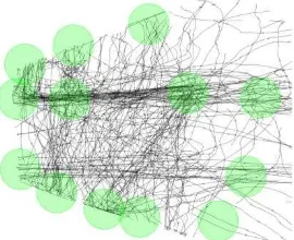
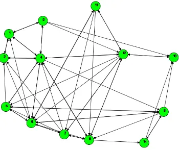
First of all we give an impression on how the results look like during the runtime. For this purpose, we use a video tracking dataset recorded in the main hall of the Leibniz University of Hannover. There 213 trajectories (10955 tracking points) of walking people have been tracked for about 30 minutes. In Figure 3 the results of the first step are shown: 14 places (nodes) have been found; they correspond to locations, where the people stopped (or reduced their speed) and where they entered or exited the observation area. Figure 4, shows the generated graph structure.
Figure 3: The extracted interesting places are results of the first step.
Figure 4: The graph structure generated from the extracted places and the segmented trajectories.
4.1 Evaluation of prediction quality
During the runtime the probabilities for all possible targets are calculated. In Figure 5 a typical prediction scenario is shown. The grey circle, which represents a moving individual, has followed the black trajectory and has entered an interesting place (green circle). Now several possible targets are determined and evaluated by probabilities. They are visualized by pairs of grey dashed lines and values.
Figure 5: Visualisation of the results of the prediction step: dashed lines point at the possible targets, values describe the
current probabilities
Since these algorithms work incrementally, we are supposing that the completeness and correctness values of an earlier stage of the runtime are worse than those at a later stage. This is motivated by the fundamental idea that there is an underlying structure in the environment, which gets visible in the data and which applies for at least a certain time. While in the early stage, a kind of 'learning stage', the model has to be built up, in the later stage, which starts after the dominant graph structure has been found, only small changes to the structure of the existing prediction model appear. Because of these different runtime stages, we divide the whole processing into smaller stages, which are evaluated incrementally. Further, we are comparing the results including all prediction factors and every factor individually. In this way, we get more significant values for the completeness C and the correctness R. In the experiments, equal weights have been set for the four factors.
The results of this evaluation are presented in Table 1. The first two stages (comprising approx. 1/3 of the data set) are considered as training, whereas the next two stages, each of which also comprises approx. 1/3 of the data set, are taken as test data. Note, however, that strictly speaking, there is no clear learning phase, as the system constantly adapts its knowledge. The completeness increases from about 31% in stage 1 to about 92% in the last stage, which is quite satisfying. The correctness for all evaluated scenarios also increases to a maximum of 44%. So, nearly a half of all predictions is correct. However, there is a slight decrease in stage 3. This may result from the change of the behavior of the objects the dataset. So the test dataset, which is used in stage 3 and 4, may contain a slightly different movement behavior. Since there is an increase in stage 4, the model seems to have adapted to this change. A possible reason for the change in the movement behavior can be the advanced time, the dataset has been recorded. At that time the intention of the users for crossing the observed area may have changed. The correctness values were calculated at each time step a trajectory point was measured. Thus, there are positions, where the prediction is less reliable than at others, e.g. at the start node it is probably less clear, where the object is heading at than closer to the end node. A closer look at the correctness can be made by dividing the segments into three parts. This information is visualized by Figure 6. There, an increase of the prediction reliability to a maximum of about 60% is recognizable during the three parts and during the four stages. This is in conformance with the average correctness of approx. 40%.
Figure 6: The average correctness development during the three parts of a segment
After evaluating the correctness of the predictions using all factors at the same time, we have also examined each factor independently (cf. Table 1). The resulting values behave similar during the stages, which, however, are below the corresponding integrated values. In this example, the neighborhood- and the history-factor provide the best results. This may change for other scenarios, where the significance of each factors differs. Finally, the results can be improved by combining and weighting those factors.
4.2 Transfer to other data sets
We developed this approach as general as possible, so that it can be used for other evaluation scenarios as well. This contains a change of input data, which may be provided by another tracking device like GPS, or a change of the use case, on which this kind of system is applied to. Besides the observation of human beings, an observation of traffic or animals is also conceivable. We want to demonstrate the portability by showing another example. This example contains an extract of a dataset, which has been collected by some students taking part at a GPS game during a summer school in Genth, Belgium (2011). The
0 0.1 0.2 0.3 0.4 0.5 0.6 0.7
1st 2nd 3rd
Stage 1
Stage 2
Stage 3
Stage 4 ISPRS Annals of the Photogrammetry, Remote Sensing and Spatial Information Sciences, Volume I-2, 2012
Stage 1 Stage 2 Stage 3 Stage 4
Description Early training Late training Early test Late test
# tracking points 1939 1939 3538 3539
Completeness C (total) 31.37% 85.96% 91.32% 91.92%
Correctness R (total) 18.02% 43.89% 40.40% 43.54%
R (Neighborhood factor) 17.69% 36.87% 34.78% 42.64%
R (Distance factor) 18.97% 43.53% 30.30% 34.26%
R (Shape factor) 18.72% 39.26% 23.86% 28.17%
R (History factor) 15.02% 40.01% 33.34% 37.78%
Table 1: Evaluation of the completeness (C) and correctness (R) of the prediction based on the video tracking datasets
dataset consist of 11 long trajectories (9627 tracking points). It shows different routes through the city taken by the participants.
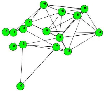
Most of the extracted places represent either meetings of different groups or road junctions, where the participants stayed for a certain time to plan where to go next. Due to the fact that a GPS tracking result is less accurate than a video tracking result, the size of the places (they are shown in Figure 7) has been enlarged. This adjustment has been necessary to receive a usable prediction basis, i.e. the graph structure, which is illustrated in Figure 8.
A similar evaluation method like the one before provides the following results (cf. Table 2).
Early stage Late stage # tracking points 4703 4924
C (total) 26.48% 89.66%
R (total) 28.08% 40.91%
Table 2: Evaluation the completeness and correctness of the prediction based on the GPS-game dataset
Again, the results are examined at an early and a late progress stage. The determined values behave similar to the values of the first test results. Here, a completeness of about 90% and a correctness of 41% are reached.
Figure 7: The extracted interesting places of the GPS game dataset...
Figure 8: ...and the corresponding graph structure
Besides the portability another required feature of this approach is the ability to use it at real-time. Due to the fact that this approach consists of two consecutive incremental steps, we examined the performance for both steps individually. Since the major effort is used by the first step (the graph building step), we are focusing on this step. When analyzing the performance it can be observed that there are also two different performance behaviors of this algorithm. Those can be referred to the different runtime stages. During the 'learning stage', in which the graph structure is built up, the processing rate decreases while the number of places increases. In the second stage just small changes of the structure appear. There, mainly the visit numbers of places are updated and new segments are added to existing segment clusters. The processing rate during this stage increases to a nearly constant level close to the start level.
5. CONCLUSION AND OUTLOOK
In summary, an approach has been presented that allows predicting movements of individuals based on path calculations within a graph structure using probability statements. The computation of the latter is composed by different components which include the knowledge about the movement behavior. The used algorithms work in real-time and on trajectory data measured by different kinds of tracking devices, which have to meet the requirements of a sufficiently high density and sampling rate. In the paper, it is applied to the observation of human beings acquired by video- and GPS-tracking.
Nevertheless, some aspects are not or not fully considered in this approach, which may further increase the prediction reliability. The most obvious one is the fact that the time aspect, which certainly influences the movement behavior of the observed individuals. A consideration of e.g. different day times
may lead to day time dependent graphs. Thus, same situations lead to different predictions at different times.
Besides that, the weighting factors have to be set at the beginning, which demands a priori knowledge about the scenario. An auto-fitting or learning possibility could be a solution for this problem. For this purpose, the graph structure
and each prediction factor’s significance can be analyzed, so
that conclusions regarding the optimal weight values can be drawn. For instance, if there is a graph structure, which is similar to a regular grid, the distances to possible targets will
not differ significantly. Thus, the prediction factor’s weight will
have to be decreased, while the other factors will have to be increased respectively.
Furthermore, we plan to examine additional prediction factors (such as the straightness or good-continuation of the path) and, instead of summing them up, further possibilities to combine those. Both may increase the prediction reliability.
Up to now we did not investigate, when the graph structure of the situation is consolidated and established. We merely divided the data sets into different stages. It will be another issue for future work to research, whether it is possible to automatically determine, when the graph is more or less established with its main components and only minor adaptations will be made. From this stage on, we assume that the correctness values of the predictions will increase. When we are able to determine this stage, the reliability of the predictions will also increase. Thus future research has to investigate, if measures can be provided, which determine, when a certain situation is stable, and when it starts changing to a new situation.
Since our motivation in developing this approach has been originated by implementing a smart camera network and the fields of view of the cameras cover just a section of the observed area, the algorithms ultimately have to work in a decentralized fashion, where the individual cameras have to cooperate. For this purpose, they have to share the prediction knowledge gained by this approach. So a camera has to inform the corresponding neighbor when an individual leaves its field of view.
6. REFERENCES
Akinori Asahara, Kishiko Maruyama, Akiko Sato, and Kouichi Seto. 2011, Pedestrian-movement prediction based on mixed Markov-chain model. In Proceedings of the 19th ACM SIGSPATIAL International Conference on Advances in Geographic Information Systems (GIS '11). ACM, New York, NY, USA, 25-33.
Ashbrook, D. and Starner, T., 2003, Using GPS to learn significant locations and predict movement across multiple users, Personal & Ubiquitous Computing 7: 275-286.
Baiget, P., Sommerlade, E., Reid, I., and Gonzàlez, J., 2008, Finding prototypes to estimate trajectory development in outdoor scenarios. In Proceedings of the First International Workshop on Tracking Humans for the Evaluation of their Motion in Image Sequences (THEMIS2008), September
Buchin, K, M. Buchin, M. van Kreveld, J. Luo, 2011, Finding long and similar parts of trajectories, Computational Geometry, Volume 44, Issue 9, November 2011, Pages 465-476.
Feuerhake, U., Kuntzsch, C., and Sester M., 2011, Finding interesting places and characteristic patterns in spatiotemporal trajectories, 8th LBS Symposium 2011, Vienna.
Helbing, D. and Molnár P., 1995, Social force model for pedestrian dynamics Physical Review E, 51 (5) (1995), pp. 4282–4286
Makris, D. and Ellis, T., 2002, Spatial and probabilistic modeling of pedestrian behavior, in Proc. Brit. Machine Vision Conf., vol. 2, Cardiff, U.K., pp. 557–566.
Schmid, F., Richter, K.-F., and Laube, P., 2009, Semantic Trajectory Compression, in Proceedings of Advances in Spatial and Temporal Databases, 11th International Symposium, SSTD 2009, Aalborg, Denmark, July 8-10, pp. 411–416.
Acknowledgements The funding of this research by DFG is gratefully acknowledged.