Splines and Radial Functions
C. Dagnino - V. Demichelis - E. Santi
ON OPTIMAL NODAL SPLINES AND THEIR APPLICATIONS
Abstract. We present a survey on optimal nodal splines and some their applications. Several approximation properties and the convergence rate, both in the univariate and bivariate case, are reported.
The application of such splines to numerical integration has been con-sidered and a wide class of quadrature and cubature rules is presented for the evaluation of singular integrals, Cauchy principal value and Hadamard finite-part integrals. Convergence results and condition number are given. Finally, a nodal spline collocation method, for the solution of Volterra integral equations of the second kind with weakly singular kernel, is also reported.
1. Introduction
It is well known that the polynomial spline approximation operators for real-valued functions are of great usefulness in the applications.
In their construction, it is desirable to obtain some nice properties as in particular: 1. the operator can be applied to a wide class of functions, including, for example,
continuous or integrable functions;
2. they are local in the sense that can depend only on the values of f in a small neighbourhood of the evaluation point x ;
3. the operators allow to approximate smooth functions f with an order of accu-racy comparable to the best spline approximation. The key for obtaining oper-ators with such property is to require that they reproduce appropriate class of polynomials.
The approximating splines obtained by applying the quasi-interpolatory operator defined in [24] satisfy the above properties and, recently, they have been widely used in the construction of integration formulas and in the numerical solution of integral and integro-differential equations, see, for instance, [3,4,7,10,13,22,27,23,28,30,32] and references therein.
This review paper is concerning the optimal nodal spline operators that, besides the properties 1., 2., 3., have the advantage of being interpolatory. These splines, in-troduced by DeVilliers and Rohwer [17,18] and studied in [12,14,16,19], have been
utilized for constructing integration rules for the evaluation of weakly and strongly singular integrals also defined in the Hadamard finite part sense, in one or two dimen-sions and, more recently, for a collocation method producing the numerical solution of weakly singular Volterra integral equations.
In Section 2., after a brief outline of the construction of one-dimensional nodal spline operators, we shall present the tensor product of optimal nodal splines, recalling also some convergence results.
Section 3. is devoted to the application of the nodal spline operators in the approx-imation of different kind of 1D or 2D integrals and the main convergence results of the corresponding integration formulas are reported.
Finally, Section 4. deals with a collocation method, based on nodal splines, for the numerical solution of linear Volterra equation with weakly singular kernel.
2. Optimal nodal splines and their tensor product
2.1. One dimensional nodal splines
Let J =[a,b] be a given finite interval of the real lineR, for a fixed integer m≥3 and n≥m−1, we define a partition5nof J by
5n: a=τ0< τ1< ... < τn=b,
generally called “primary partition”. We insert m −2 distinct points throughout (τν, τν+1),ν=0, ...,n−1 obtaining a new partition of J
Xn: a=x0<x1, < ... <x(m−1)n=b, where x(m−1)i=τi, i=0, ...,n. Let
(1) Rn= max
0≤k,j≤n−1
|k−j| =1
τk+1−τk τj+1−τj ,
we say that the sequence of partitions{5n;n =m−1,m, ...}is locally uniform (l.u.) if, for all n, there exists a constant A≥1 such that Rn ≤A, i.e.
(2) 1
A ≤
τk+1−τk τj+1−τj
≤ A, k,j =0,1, ...,n−1 and|k− j| =1.
Since the convergence results of the nodal splines we shall consider are based on the local uniformity property of the primary partitions sequence and one of our objectives is the use of graded meshes, the following proposition shows that a sequence of primary graded partitions is l.u. [8]. For the definition of graded partitions see for example [2]. PROPOSITION1. Let [a,b] be a finite interval. The sequence of partitions{5n}, obtained by using graded meshes of the form
τi =a+
i
n
r
with grading exponent r∈Rassumed≥1, is l.u., i.e. it satisfies (2) with A=2r −1. Now, after introducing two integers [16]
i0=
αi,r,j are given in [19] and the B-spline sequence is constructed from the set of the normalized B-splines for i =(m−1)(i1−2),(m−1)(i1−2)+1, ..., (m−1)(n−i0+1).
Then, the following locality property holds [17]
(4) si(x)=0 , x 6∈[τi−i0, τi+i1].
Therefore, being det[wi(τj)] 6=0, the functionswi(x),i =0,1, . . . ,n,are linearly independent. Let S5n =span{wi(x);i =0,1, ...,n}, it is proved in [18] that, for all
s∈S5n, one has s ∈Cm
−2(J).
For all g∈B(J), where B(J)is the set of real-valued functions on J , we consider the spline operator Wn: B(J)→S5n, so defined
Wng= n
X
i=0
g(τi)wi(x) , x∈ J.
By (4), for 0≤ν <n we can write:
(5) Wng =
qν X
i=pν
g(τi)wi(x), x ∈[τν, τν+1].
Moreover Wnp = p, for all p ∈ Pm ,wherePm denotes the set of polynomials of order m (degree≤ m−1), and Wng(τi) = g(τi), for i = 0,1, ...,n, i.e. Wn is an interpolatory operator [17,18].
Using the results in [17-19] we deduce that, for l.u.{5n}, Wnis a bounded projec-tion operator in S5n. In fact, it is easy to show that
Wns=s , for all s∈S5n
and, if we denote:
||Wn|| =sup{||Wnh||∞: h∈C(J),||h||∞<1}, with||h||∞=max
x∈I |h(x)|, considering that
||Wn|| ≤(m+1)
"m−1
X
λ=1
(Rn)λ
#m−1
,
where Rnis defined in (1), from (2), if{5n}is l.u., we obtain||Wn||<∞.
We remark that if we assume the (m −2) points equally spaced throughout (τν, τν+1), ν = 0,1, . . . ,n −1, then the local uniformity constant of{Xn}will be equal to that of{5n}.
Finally for all g∈Cs−1(J), with 1≤s≤m, we introduce the following quantity Eνs =
Dν(g−Wng) , 0≤ν <s DνWng , s≤ν <m. If{Xn}is l.u., for 0≤ν≤s−1 there results [14,19]
(6) ||Eνs||∞=O Hns−ν−1ω(Ds−1g;Hn;J) where
(7) Hn= max
and for all f ∈C(J), ω(f;δ;J)= max
x,x+h∈J
0<h≤δ
|f(x+h)− f(x)|. For s≤ν <m in [14] a bound for|Eνs|is given.
Furthermore, for every t⊆ J and g∈Cν(J), 0≤ν <m−1 [27] ω(DνWng;t;J)=O ω(Dνg;t;J).
2.2. Tensor product of optimal nodal splines
Let D be theR2subset defined by [a,b]×[a,˜ b].˜ We consider partitions5nand Xn on which we construct the spline functions of order m{wi(x),i =0, . . . ,n}defined in ( 3 ).
Then we consider similar partitions of [a,˜ b],˜ 5˜n˜ and X˜n˜ and we construct the corresponding functions of orderm˜ { ˜w˜i(x),˜ ˜i =0, . . . ,n˜}.
Now we may generate a set of bivariate splines wi,˜i(x,x)˜ =wi(x)w˜i(x)˜ tensor product of the (3) ones.
Let B(D)denote the set of bounded real-valued functions on D. Then, for any f ∈ B(D)we may define the following spline interpolating operator for (x,x)˜ ∈
[τj, τj+1]×[τ˜j˜,τ˜˜j+1],
(8) Wn∗n˜f(x,x)˜ = qj X
i=pj
˜ qj X
˜ i= ˜pj˜
wi,˜i(x,x)˜ f(τi,τ˜˜i),
with j=0,1, . . . ,n−1 and ˜j=0,1, . . . ,n˜−1.
In order to obtain the maximal order polynomial reproduction, we can assume m= ˜
m, i.e. we use splines of the same order on both axes. We list in the following the main properties of Wn∗n˜.
(a) Wn∗n˜ is local, in the sense that Wn∗n˜f(x,x˜)depends only on the values of f in a small neighbourhood of(x,x);˜
(b) Wn∗n˜interpolates f at the primary knots, i.e. Wn∗n˜f(τi,τ˜˜i)= f(τi,τ˜˜i);
(c) Wn∗n˜ has the optimal order polynomial reproduction property, that means Wn∗n˜p =
p, for all p∈P2m, whereP2m is the set of bivariate polynomials of total order m. For f ∈Cs−1(D),1≤s<m we introduce the following quantity
Eνν˜s =
where Dν,ν˜ is the usual partial derivative operator.
Now we say that a collection of product partitions{Xn× ˜Xn˜}of D is quasi uniform (q.u.) if there exists a positive constantσ such that
1
ˆ
δ, 1
˜
δ,
˜
1
ˆ
δ,
˜
1
˜
δ ≤σ ,
where1 = max1≤i≤n(m−1)(xi −xi−1), δˆ = min1≤i≤n(m−1)(xi −xi−1)and1˜ =
max1≤˜i≤ ˜n(m−1)(x˜˜i − ˜x˜i−1), δ˜=min1≤˜i≤ ˜n(m−1)(x˜˜i − ˜x˜i−1). We set
(9) H∗=Hn+ ˜H˜n and 1∗=1+ ˜1
where Hnis defined in ( 7 ) and likewiseH˜˜n.
Assuming that f ∈ Cs−1(D)with 1≤s <m and that{Wnn˜f}is a q.u. sequence of nodal splines, then forν,ν˜such that 0≤ν+ ˜ν ≤s−1
||Eνν˜s||∞=O H∗s−ν− ˜ν−1ω(Ds−1f;H∗;D).
In [9] local bounds of|Eνν˜s|are derived and local and global bounds of|Eνν˜s|, s ≤ ν+ ˜ν <m, are also given.
Furthermore, for f ∈Cp(D), 0≤ p<m−1, and for a q.u. sequence of nodal splines{Wn∗n˜f}, there results for any non empty subset T of D
ω(DpWn∗n˜f;T;D)=O ω(Dpf;T;D).
In the following we shall consider l.u. partitions in the one dimensional case and q.u. partitions in the 2D one and we shall suppose always that the norm of the partitions converges to zero as n→ ∞or n,n˜ → ∞.
3. Numerical integration based on nodal spline operators
This section will deal with the numerical evaluation of some singular one-dimensional integrals and of certain 2D singular integrals.
3.1. Product integration of singular integrands
Consider integrals of the form
(10) J(k f)=
Z
I
k(x)f(x)d x
where k f ∈L1(I), but f is unbounded in I =[−1,1].
By using (6) withν =0, the author gets, firstly, the convergence of the quadrature sum J(kWnf), i.e.:
(11) J(kWnf)→ J(k f)as n→ ∞ by supposing f ∈C(I), k∈L1(I)and Hn→0 as n→ ∞.
We recall that a computational procedure to generate the weights {vi(k) =
R
Ik(x)wi(x)d x}of the above quadrature is given in [6].
Moreover in [26] the case when f ∈PC(I), k∈ L1(I)is studied and the
conver-gence of the quadrature rules sequence is proved.
We remark that in [11] the convergence (11) has been proved also for f ∈ R(I), the class of Riemann integrable functions on I and k∈L1(I).
When the function f in (10) is singular in z ∈ [−1,1)in [25] the author defines the family of real valued functions Md(z;k):
(12)
Md(z;k)= {f : f ∈PC(z,1],∃F : F=0 on [−1,z],F is non negative, continuous
and nonincreasing on(z,1),k F∈L1(I)and|f| ≤F on I}
.
He supposes that k satisfies one of the following conditions A,B:
(A) There existsδ >0 :|k(x)| ≤K(x),∀x ∈(z,z+δ], K is positive nonincreasing in that interval and K F, F defined in (12), is a L1function in I .
(B) Given q0∈(0,1),∃δ,T , positive numbers (possibly depending on q0), such that
Z c+h
c
|k(x)|d x≤hT|k(c+qh)|
∀q ∈[q0,1],∀c and h satisfying z≤c<c+h≤z+δ. Besides|k(x)f(x)| ≤
G(x),∀x ∈ (z,z+δ], where G is a positive non increasing L1function in that
interval.
The following theorem can be proved.
THEOREM 1. Assume that f ∈ Md(−1;k)and k satisfies (A) or (B). If the se-quence of partitions{5n}is l.u. and the norm converges to zero as n→ ∞, then (11) holds.
As consequence of that theorem if z= −1 the singularity can be ignored, provided k satisfies (A) or (B).
In the case when z is an interior singularity, it must, in general, be avoided, i.e. we must define a new integration rule
J∗(kWnf)= n
X
i=J
where J is the smallest integer such that z≤τJ−λ, whereτJ−λis the left bound of the
support of sJ(x)and, if we assume that n is so large that J ≥ m, thenwi =si and vi(k)is given by:
vi(k)=
Z τi+µ
τi−λ
k(x)si(x)d x, withλ=i0andµ=i1.
Therefore, assuming that f ∈ Md(z;k),z > −1, and k satisfying (A) or (B). If {5n}is locally uniform and the norm tends to zero as n→ ∞, then
J∗(kWnf)→ J(K f) as n → ∞.
If one wishes to use J(kWnf)rather than J∗(kWnf) then k must be restricted in [−1,z)as well as in(z,1], for satisfying one of the following conditions(A)ˆ or(B).ˆ (A)ˆ : (A) holds and, in addition,|kz(x)| ≤ K(x)in(z,z+δ], where kz ∈ L1(2z−
1,2z+1)is defined by kz(z+y)=k(z−y). (B)ˆ : (B) holds and so does (B) with k replaced by kz.
THEOREM2. Let f ∈ Md(z;k),z >−1. Assume that k satsfies(A)ˆ or(B)ˆ and that{5n}is l.u. and the norm converges to zero as n→ ∞.
Define
ˆ
J(kWnf)=J(kWnf)−vρf(τρ)
whereτρis the value ofτi ≥z closest to z. Then ˆ
J(kWnf)→ J(k f) as n → ∞.
In particular, ifτρ =z then (11) holds. If z is such that for all n, τρ−z>C(τρ−τρ−1),
then (11) holds.
3.2. Cauchy principal value integrals
Consider the numerical evaluation of the Cauchy principal value (CPV) integrals (13) J(k f;λ)=
Z 1
−1
−k(x) f(x)
x−λd x, λ∈(−1,1).
In [11] the problem has been investigated, following the “subtracting singularity” ap-proach.
Assuming that J(k;λ)exists forλ∈(−1,1), the integral (13) can be written in the form
J(k f;λ) =
Z 1
−1
where
gλ(x)=g(x;λ)=
f(x)−f(λ)
x−λ x6=λ
f′(λ) x=λand f′(λ)exists
0 otherwise.
Therefore, approximatingI(kgλ)byI(kWngλ)we can write [11]
J(k f;λ)=Jn(k f;λ)+En(k f;λ), where
Jn(k f;λ)=I(kWngλ)+ f(λ)J(k;λ) .
For anyλ∈(−1,1)we define a family of functionsM¯d(z;k)= {g∈C(I\λ),∃G : G is continuous nondecreasing in [−1;λ), continuous non increasing in (λ,1];kG ∈
L1(I),|g|<G in I}.
We assume
Nδ(λ)= {x :λ−δ≤x≤λ+δ},
whereδ >0 is such that Nδ(λ)⊂I .
We denote by Hµ(I),µ∈(0,1], the set of H¨older continuous functions
Hµ(I) = {g∈C(I):|g(x1)−g(x2)| ≤ L|x1−x2|µ,∀x1,x2∈I,L>0}
and by DT(I)the set of Dini type functions
DT(I)= {g∈C(I):
Z l(I)
0
ω(g;t)t−1dt<∞}
where l(I)is the length of I andωdenotes the usual modulus of continuity.
The following convergence results for the quadrature rules Jn(k f;λ), under differ-ent hypotheses for the function f , are derived in [11].
THEOREM 3. For anyλ ∈ (−1,1), let f ∈ H1 Nδ(λ)∩R(I)and k ∈ L1(I).
Then, for l.u.{5n}, En(k f;λ)→0 as n→ ∞.
THEOREM4. Let f ∈Hµ(I), 0< µ <1, k∈L1(I)∩C Nδ(λ). Let h and p be
the greatest and the smallest integers such thatτh < λ,τp> λ. We denote byτ∗the node closest toλ
τ∗=
τh if λ−τh ≤τp−λ τp if λ−τh > τp−λ and we suppose that there exists some positive constant C, such that
|τ∗−λ|>C max{(τh−τh−1), (τp+1−τp)}, then, for l.u.{5n},
THEOREM5. Let f ∈C1(I), k∈L1(I). Then
3.3. The Hadamard finite part integrals
We consider the evaluation of the finite part integrals of the form
(14) J¯(ωα,βf)=
=denotes the Hadamard finite part (HFP). It is well known that a sufficient condition so that (14) exists is
f ∈Hµ(I), 0< µ≤1, µ+β >0.
whereŴis the gamma function.
where
¯
Jn(f)= n
X
i=0 ¯
vi(ωα,β)f(τi)
withv¯i(ωα,β)= ¯J(ωα,βwi), and ¯
En(f)= ¯J(ωα,β(f −Wnf)).
A computational procedure for evaluatingv¯i(ωα,β)is given in [6].
Denoting by Hsµ(I)the set of the functions f ∈Cs(I)having f(s)∈Hµ(I), in [5]
the following theorem has been proved.
THEOREM6. Let f ∈Hsµ(I), 0≤s≤m−1, andµ+β >0 if s=0. Then, as n→ ∞:
|| ¯En(f)||∞=
(
O(Hns+µ+β) ifβ <0 O(Hns+µ|log Hn|) ifβ =0. Consider now HFP integrals of the form:
(17) J∗(ωα,βf;λ;p)=
Z
I
= ωα,β(x)
f(x)
(x−λ)p+1, λ∈[−1,1], p≥1
If f ∈Hµp(I), then J∗(ωα,βf;λ;p)exists.
In [20, 21] quadrature rules for the numerical evaluation of (17), based on some dif-ferent type of spline approximation, including the optimal nodal splines, are considered and studied.
In [29] the following theorem has been proved.
THEOREM7. Assume that in (17)λ∈(−1,1), p∈N and f ∈ Hµp. Let{fn}be a given sequence of functions such that fn∈Cp(I)and
i) - ||Djrn||∞=o(1) as n→ ∞ j =0,1, . . . ,p, where rn= f − fn ii) - Djrn(−1)=0 0≤ j≤ p−β; Djrn(1)=0 0≤ j≤ p−α iii) - rn∈Hσp(I), ∀n, 0< σ ≤µ, σ+min(α, β) >0.
Then
(18) J∗(ωα,βfn;λ;p)→ J∗(ωα,βf;λ;p) as n→ ∞
uniformly for∀λ∈(−1,1).
Therefore, in [15], for 0≤s, t ≤ p, are defined two sets of B-splines B¯i,B¯N−i on the knot sets
{x0, . . .x0,x1, . . . ,xs+1}, {xN−t−1, . . . ,xN−1,xN, . . . ,xN} respectively, where N =(m−1)n and x0,xN are repeated exactly m times.
Considering that Wnf(τi)= f(τi), i=0,n, one defines
gn(x):=
Ps
i=1diB¯i(x) x∈[x0, . . . ,xs+1]
0 x∈(xs+1, . . . ,xN−t−1)
Pt
i=1d˜iB¯N−i(x) x∈[xN−t−1, . . . ,xN]
where di,d˜i are determined by solving two non-singular triangular systems obtained by imposing
g(j)(τ0)=rn(j)(τ0) j =1,2, . . . ,s
gn(j)(τn)=rn(s)(τn) j =1,2, . . . ,t
For the sequence{ ˆWnf =Wnf +gn}, it is possible to prove the following: THEOREM8. Let{ ˆWnf}be a sequence of modified optimal nodal splines and set ˆ
rn = f − ˆWnf , then ˆ
Wnf(τi)= f(τi) i =0, . . . ,n;
Djrˆn(−1)=0, 0≤ j≤ p−β; Djrˆn(1)=0, 0≤ j ≤ p−α, ˆ
Wng=g if g∈Pm.
Besides supposing f ∈Cr(Ik), Ik =[τk, τk+1], hk =τk+1−τk, for any x ∈ Ikthere results:
|Dνrˆn(x)| ≤ ˜kνhrk−νω(Dr f;hk;Ik), ν=0, . . . ,r |Dr+1Wˆnf(x)| ≤ ˜kr+1h−k1ω(Drf;hk;Ik),
ˆ
rn ∈Hrµ(I).
Therefore all the conditions of theorem 3.3.2 being satisfied, ifµ+min(α, β) >0, then
J∗(ωα,βWˆnf;λ;p)→ J(ωα,βf;λ;p) as n→ ∞
uniformly for∀λ∈(−1,1).
3.4. Integration rules for 2-D CPV integrals
In this section we will consider the numerical evaluation of the following two types of CPV integrals:
(19) J1(f;x0,y0)=
Z
R
−ω1(x)ω2(y)
f(x,y) (x−x0)(y−y0)
where R=[a,b]×[a,˜ b], x˜ 0∈(a,b), y0∈(a,˜ b), and we assume˜ ω1(x)∈L1[a,b]∩
where D denotes a polygonal region and 8(P0,P)is an integrable function on D
except at the point P0where it has a second order pole.
For numerically evaluating (19), in [9] the following cubatures based on a sequence of nodal splines ( 8 ) have been proposed:
J1(Wnn˜f;x0,y0)=
We denote by Hµ,µp (R)the set of continuous functions having all partial derivatives
of order j =0, . . . ,p,p ≥ 0 continuous and each derivative of order p satisfying a H¨older condition, i.e.:
|f(p)(x1,y1)− f(p)(x2,y2)| ≤C(|x1−x2|µ+ |y1−y2|µ), 0< µ≤1
for some constant C>0, and we assume
(21) Enn˜(f;x0,y0)=J1(f;x0,y0)−J1(Wnn˜f;x0,y0).
In [9] the following convergence theorem has been proved.
THEOREM9. Let f ∈Hµ,µp , 0< µ≤1, 0≤ p<m−1. For the remainder term
in (21), there results:
Enn˜(f;x0,y0)=O (1∗)p+µ−γ,
whereγ ∈R, 0< γ < µ, small as we like and1∗has been defined in (9).
In many practical applications it is necessary that rules, uniformly converging for
∀(x0,y0)∈(−1,1)×(−1,1), are available, in particular considering the Jacobi weight
type functions
ω1(x)=(1−x)α1(1+x)β1, ω2(y)=(1−y)α2(1+y)β2
withαi, βi >−1, i=1,2,(x,y)∈ R=[−1,1]×[−1,1].
In order to obtain uniform convergence for approximating rules numerically evalu-ating (19), can be useful to write the integral in the form
where J(ω1;x0)=
Z 1
−1 − ω1(x)
x−x0
d x, J(ω2;y0)=
Z 1
−1 − ω2(y)
y−y0
d y.
We exploit the results in [31] where, considering a sequence of linear operators Fnn˜ approximating f , the integration rule for (22):
J1(Fnn˜;x0,y0) =
Z
R
− ω1(x)ω2(y)
Fnn˜(x,y)−Fnn˜(x0,y0)
(x−x0)(y−y0)
d x d y
+ f(x0,y0)J(ω1;x0)J(ω2;y0)
has been constructed. Denoting rnn˜ = f −Fnn˜, and 1nn˜ the norm of the partition, with lim
n→ ∞
˜
n→ ∞
1nn˜=0, the following general theorem of uniform convergence has been proved.
THEOREM10. Let f ∈ Hµµ0 (R), and assume that the approximation Fnn˜ to f is such that
i) rnn˜(x,±1)=0 ∀x ∈[−1,1],rnn˜(±1,y)=0 ∀y∈[−1,1], ii) ||rnn˜||∞=O(1νnn˜), 0< ν≤µ,
iii) rnn˜ ∈Hσ0(R), 0< σ≤µ.
Ifρ+γ− ¯ε >0, whereρ=min(σ, ν), γ =min(α1, α2, β1, β2)andε¯is a positive
real number as small as we like, then, for the remainder term, Enn˜ = J1(f;x0,y0)−
J1(Fnn˜;x0,y0), there results:
Enn˜(f;x0.y0)→0 as n→ ∞,n˜→ ∞
uniformly for∀(x0,y0)∈(−1,1)×(−1,1).
If we consider Fnn˜ =Wnn˜(f;x,y)only the conditions ii), iii), with1n,n˜ =1∗, are satisfied, but we can modify Wnn˜in the form
¯
Wnn˜(f;x,y) =Wnn˜(f;x,y)+[ f(−1,y)−Wnn˜(f; −1,y)]B1−m(x) +[ f(1,y)−Wnn˜(f;1,y)]B(m−1)n−1(x)
+[ f(x,−1)−Wnn˜(f;x,−1)]B˜1−m(y) +[ f(x,1)−Wnn˜(f;x,1)]B(m−1)n˜−1(y) .
Assumingr¯nn˜(x,y) = f(x,y)− ¯Wnn˜(f;x,y), all the condition i)−i i i)are verified and then
J1(W¯nn˜;x0,y0)→ J1(f;x0,y0) as n,n˜→ ∞
uniformly for∀(x0,y0)∈(−1,1)×(−1,1).
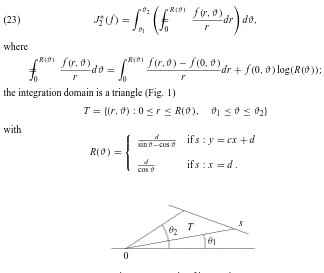
at one vertex, by introducing polar coordinates(r, ϑ)with origin at the singularity P0,
the evaluation of (20) can be reduced to the evaluation of
(23) J2∗(f)= the integration domain is a triangle (Fig. 1)
T = {(r, ϑ): 0≤r≤ R(ϑ), ϑ1≤ϑ ≤ϑ2}
Figure 1. Domain of integration T .
Let us assume R =maxϑ∈[ϑ1,ϑ2]|R(ϑ)|,R=[0,R]×[ϑ1, ϑ2] and define m
∗ = min(m,m).¯
We can prove the following theorem:
THEOREM11. If f ∈ Hsµ,µ(R) , 0 < µ≤ 1 and 0 ≤ s ≤ m∗−1, {5n}and { ¯YN}are sequence of locally uniform partitions, then
||Rn,N(f)||∞=O(H¯s +µ
N |log(H¯N)| +H s+µ−ε
n )
whereεis a positive real as small as we like.
4. A collocation method for weakly singular Volterra equations
Consider the Volterra integral equation of the second kind
(24) y(x)= f(x)+
Z x
0
k(x,s)y(s)ds x∈I ≡[0,X ]
where k is weakly singular kernel, in particular of convolution type of the form k(x−s), where k∈C(0,X ]∩L1(0,X), but k(t)can become unbounded as t→0.
In [8], for numerically solving (24) a product collocation method, based on optimal nodal splines, has been constructed, for which error analysis and condition number are given.
If we consider a spline yn∈Sπn, written in the form
yn(x)= n
X
j=0
αjwj(x) αj ∈R, j =0, . . . ,n,
and we substitute such function in (24), we obtain yn(x)−
Z x
0
k(x,s)yn(s)ds+rn(x)= f(x)
where rn(x)is the residual term obtained in approximating y by yn. The valuesαj are determined by imposing
(25) rn(τj)=0 j =0, . . . ,n, i.e. as solution of a linear system of the form
αj[1−µ(τj)]− n
X
i=0
i6=j
µi(τj)αi = f(τj) j =0, . . . ,n,
whereµi(τj)=
Z τj
0
In the quoted paper the explicit form ofµi(τj)for different values of i is provided. Exploiting the properties of the operator Wn, which is a bounded interpolating pro-jection operator, the condition (25) can be rewritten in the form
(26) (I −WnK˜)yn=Wnf,
whereK y˜ =
Z
I ˜
k(x,s)y(s)ds, with
˜
k(x,s)=
k(x,s) 0≤s≤x 0 s>x,
is a bounded compact operator on C(I)[1]. Therefore we can deduce that equation (26) has a unique solution and
THEOREM12. For all n sufficiently large, say n≥N , the operator(I−WnK˜)−1 from C(I)to C(I)exists.
Moreover it is uniformly bounded, i.e.: sup
n≥N
||(I−WnK˜)−1|| ≤M <∞
and
||y−yn||∞≤ ||(I−WnK˜)−1|| ||y−Wny||∞.
This leads to||y−yn||∞converging to zero exactly with the same rate of the norm of the nodal spline approximation error.
References
[1] ATKINSONK.E., The numerical solution of integral equations of the second kind, Cambridge Mon. on Appl. Comp. Math., Cambridge University Press 33 (1997), 59–672.
[2] BRUNNERH., The numerical solution of weakly singular Volterra integral equa-tions by collocation on graded meshes, Math. Comp. 45 (1985), 417–437. [3] CALIO´ F.ANDMARCHETTIE., On an algorithm for the solution of generalized
Prandtl equations, Numerical Algorithms 28 (2001), 3–10.
[4] CALIO´ F.ANDMARCHETTIE., An algorithm based on Q. I. modified splines for singular integral models, Computer Math. Appl. 41 (2001), 1579–1588.
[6] DAGNINO C. AND DEMICHELISV., Computational aspects of numerical inte-gration based on optimal nodal spline, Intern. J. Computer Math. 80 (2003), 243–255.
[7] DAGNINO C., DEMICHELISV. ANDSANTIE., Numerical integration of singu-lar integrands using quasi-interpolatory splines, Computing 50 (1993), 149–163. [8] DAGNINO C., DEMICHELIS V. AND SANTI E., A nodal spline collocation method for weakly singular Volterra integral equations, Studia Univ. Babes-Bolyai Math. 48 3 (2003), 71–82.
[9] DAGNINOC., PEROTTOS.ANDSANTIE., Convergence of rules based on nodal splines for the numerical evaluation of certain Cauchy principal value integrals, J. Comp. Appl. Math. 89 (1998), 225–235.
[10] DAGNINO C. ANDRABINOWITZP., Product integration of singular integrands using quasi-interpolatory splines, Computer Math. Applic. 33 (1997), 59–672. [11] DAGNINOC.ANDSANTIE., Numerical evaluation of Cauchy principal integrals
by means of nodal spline approximation, Revue d’Anal. Num. Theor. Approx. 27 (1998), 59–69.
[12] DAHMENW., GOODMANT.N.T.ANDMICCHELLIC.A., Compactly supported fundamental functions for spline interpolation, Numer. Math. 52 (1988), 641– 664.
[13] DEMICHELISV., Uniform convergence for Cauchy principal value integrals of modified quasi-interpolatory splines, Intern. J. Computer Math. 53 (1994), 189– 196.
[14] DEMICHELISV., Convergence of derivatives of optimal nodal splines, J. Approx. Th. 88 (1997), 370–383.
[15] DEMICHELIS V. AND RABINOWITZ P., Finite part integrals and modified splines, to appear in BIT .
[16] DE VILLIERSJ.M., A convergence result in nodal spline interpolation, J.
Ap-prox. Theory 74 (1993), 266–279.
[17] DE VILLIERSJ.M. AND ROHWER C.H., Optimal local spline interpolants, J. Comput. Appl. Math. 18 (1987), 107–119.
[18] DE VILLIERSJ.M. AND ROHWERC.H., A nodal spline generalization of the
Lagrange interpolant, in: “Progress in Approximation Theory” (Eds. Nevai P. and Pinkus A.), Academic Press, Boston 1991, 201–211.
[20] DIETHELMK., Error bounds for spline-based quadrature methods for strongly singular integrals, J. Comput. Appl. Math. 89 (1998), 257–261.
[21] DIETHELMK., Error bounds for spline-based quadrature methods for strongly singular integrals, J. Comp. Appl. Math. 142 (2002), 449–450.
[22] GORI C. AND SANTI E., Spline method for the numerical solution of Volterra integral equations of the second kind, in: “Integral and Integro-differential equa-tion” (Eds. Agarwal R. and Regan D.O.), Ser. Math. Anal. Appl. 2, Gordon and Breach, Amsterdam 2000, 91–99.
[23] GORIC., SANTIE.AND CIMORONI M.G., Projector-splines in the numerical solution of integro-differential equations, Computers Math. Applic. 35 (1998), 107–116.
[24] LYCHET.ANDSCHUMAKERL.L., Local spline approximation methods, J. Ap-prox. Theory 15 (1975), 294–325.
[25] MONEGATOG., The numerical evaluation of a 2-D Cauchy principal value in-tegral arising in boundary inin-tegral equation methods, Math. Comp. 62 (1994), 765–777.
[26] RABINOWITZ P., Product integration of singular integrals using optimal nodal splines, Rend. Sem. Mat. Univ. Pol. Torino 51 (1993), 1–9.
[27] RABINOWITZP., Application of approximating splines for the solution of Cauchy singular integral equations, Appl. Num. Math. 15 (1994), 285–297.
[28] RABINOWITZP., Optimal quasi-interpolatory splines for numerical integration, Annals Numer. Math. 2 (1995), 145–157.
[29] RABINOWITZ P., Uniform convergence results for finite-part integrals, in: “Workshop on Analysis celebrating the 60thbirthday of Peter V´ertesi and in mem-ory of Ott`o Kis and Apard Elbert”, Budapest 2001.
[30] RABINOWITZP.ANDSANTIE., On the uniform convergence of Cauchy princi-pal values of quasi-interpolating splines, BIT 35 (1995), 277–290.
[31] SANTI E., Uniform convergence results for certain two-dimensional Cauchy principal value integrals, Portugaliae Math. 57 (2000), 191–201.
AMS Subject Classification: 65D30, 65D07.
Catterina DAGNINO, Vittoria DEMICHELIS Dipartimento di Matematica
Universit`a di Torino via Carlo Alberto 8 10123 Torino, ITALIA
e-mail:[email protected] [email protected]
Elisabetta SANTI
Dipartimento di Energetica Universit`a dell’ Aquila Monteluco di Roio 67040 L’Aquila, ITALIA