Three-Hilbert-Space Formulation
of Quantum Mechanics
⋆Miloslav ZNOJIL
Nuclear Physics Institute ASCR, 250 68 ˇReˇz, Czech Republic E-mail: [email protected]
URL: http://gemma.ujf.cas.cz/∼znojil/
Received October 29, 2008, in final form December 31, 2008; Published online January 06, 2009
doi:10.3842/SIGMA.2009.001
Abstract. In paper [Znojil M.,Phys. Rev. D 78(2008), 085003, 5 pages,arXiv:0809.2874] the two-Hilbert-space (2HS, a.k.a. cryptohermitian) formulation of Quantum Mechanics has been revisited. In the present continuation of this study (with the spaces in question denoted as H(auxiliary) andH(standard)) we spot a weak point of the 2HS formalism which lies in the
double role played byH(auxiliary). As long as this confluence of roles may (and did!) lead to
confusion in the literature, we propose an amended, three-Hilbert-space (3HS) reformulation of the same theory. As a byproduct of our analysis of the formalism we offer an amendment of the Dirac’s bra-ket notation and we also show how its use clarifies the concept of covariance in time-dependent cases. Via an elementary example we finally explain why in certain quantum systems the generator H(gen) of the time-evolution of the wave functions may
differfrom their HamiltonianH.
Key words: formulation of Quantum Mechanics; cryptohermitian operators of observables; triplet of the representations of the Hilbert space of states; the covariant picture of time evolution
2000 Mathematics Subject Classification: 81Q10; 47B50
1
Introduction
In contrast to classical mechanics where various formulations of the theory abound, there exist not too many alternative formulations of quantum theory. Moreover, most of their lists (to be found mostly in textbooks and just rarely in review papers like [1]) pay attention just to the history of the subject, creating an impression that the formulation of quantum theory does not lead to any interesting theoretical developments.
Ten years ago this false impression has been challenged by Bender and Boettcher [2] who surprised the physics community by a numerically supported conjecture that quite a few one-dimensional quantum potentials V(x) may generate bound states ψn(x) with real energies En even when the potentials themselves are not real. The conjecture seemed to contradict the current experience with quantum mechanics. Using the traditional textbook single-Hilbert-space (1HS) formulation of the theory [3] we usually employ the fact that the separable Hilbert spaces are all unitarily equivalent. This allows us to restrict attention, say, to the exceptional and most user-friendly representationsℓ2 orL2(R) of the Hilbert space of states (cf. AppendixA
for a few additional comments). On this background one can expect a complexification of the spectra whenever the underlying Hamiltonian becomes manifestly non-Hermitian. It is just this naive belief which has been shattered by the Bender’s and Boettcher’s illustrative Hamiltonians
⋆
This paper is a contribution to the Proceedings of the VIIth Workshop “Quantum Physics with Non-Hermitian Operators” (June 29 – July 11, 2008, Benasque, Spain). The full collection is available at
which all possessed, as an additional methodical benefit, the most elementary and common form
H =p2+V(x) of the sum of the kinetic and potential “energies”.
Obviously, any imaginary component inV(x) makes the latter Hamiltonians with real spectra safely non-Hermitian in L2(R). This is a paradox which evoked an intensive interest in the
families of apparently unphysical Hamiltonians H the Hermiticity of which appeared broken in a theoretically inappropriate but mathematically exceptional and friendly specific representation of an abstract Hilbert space which will be denoted here as H(auxiliary),
H 6=H† in H(auxiliary). (1) The progress in this direction of research has been communicated in dedicated conferences (cf. their webpage [4] and proceedings [5] or, better, the recent compact review paper [6]). It became clear that in spite of the undeniable appeal of the models where En = real while
V(x) = complex one must treat their “non-Hermiticity” (1) as an ill-conceived concept. The operatorsH with real spectra have been reinterpreted as Hermitian after an appropriatead hoc redefinition of the Hilbert space H of states. For this purpose one must merely replace the original, false spaceH(auxiliary)by another, physical spaceH(standard)of states with the standard quantum-mechanical meaning.
A few relevant aspects of such a theoretical and conceptual innovation will be discussed in our present paper. Our introductory Section 2 and Appendix A recollect the main features of the currently most popular two-Hilbert-space (2HS) formulation of such a version of quantum theory1 which is based on the use of the so called quasi-Hermitian or, better, cryptohermitian2 representation of observables. In Subsection 2.2, in particular, we return briefly to our recent paper [9] where the 2HS formalism has been shown suitable for the description of such quasi-Hermitian quantum systems which require the use of manifestly time-dependent operators of observables.
In Section 3 our present main result is described showing that a thorough simplification of the theory can be achieved when one replaces its 2HS formulation by a more appropriate three-Hilbert-space (3HS) reformulation. A few subtleties of the resulting generalized formalism (as well as of our present amended notation conventions) are illustrated via an elementary time-independent two-dimensional matrix solvable example in Section 4.
Section 5 returns again to the results of [9]. We stress there that one of the most remark-able applications of the innovated 3HS formalism can be found in the perceivably facilitated covariant construction of certain sophisticated generators of time evolution. For illustration we return to the matrix example of Section 4 and we re-analyze its time-dependent generalized version in Section 6. We firmly believe that the 3HS description of this and similar examples can perceivably simplify our understanding of paradoxes which may emerge in quasi-Hermitian models.
The summary of our results is provided in Section7. Several apparently anomalous properties of the Bender’s and Boettcher’s potentials are discussed there as an inspiration of revisiting a few less rigorous formulations of the first principles of quantum theory. No real necessity of the changes of these general principles themselves is encountered. Still, our present modification of their implementation and of the related conventions in notation appears both desirable and beneficial.
2
Quantum Mechanics in 2HS formulation – a brief recollection
The practical use of phenomenological Hamiltonians H which are apparently non-Hermitian (cf. (1)) does certainly enhance the flexibility of the constructive model-building activities in
physics even behind the framework of quantum theory (cf. [10]). It also broadens the space for feasible applications of non-local models in a way exemplified by the above-mentionedcomplex Bender–Boettcher toy potentials [6]. In similar cases, an attachment of the doublet of Hilbert spacesH(auxiliary) and H(standard) to a single quantum system may make good sense.
2.1 The hermitization of cryptohermitian observables
One of the first applications of the apparently non-Hermitian Hamiltonians with real spectra appeared in nuclear physics [7]. The correct physical interpretation of the model in H(standard) has been separated there from thefacilitated calculationsof the spectrum inH(auxiliary). Further physical application of the same method appeared in Mostafazadeh’s study of the free relativistic Klein–Gordon equation [11] which is traditionally introduced in the Feshbach’s and Villars’ [12] unphysical representation space H(auxiliary) = L2(R)L
L2(R). A reconstruction of the
inner product has been offered as a means of recovering the consistent picture of physics. The same approach avoiding spurious states or negative probabilities has been extended to the first-quantized models of massive particles with spin one [13].
On theoretical level the 2HS reformulation of quantum theory might look almost trivial. Still, the application of the idea to the Bender’s and Boettcher’s elementary examples and the resolution of some of the related puzzles took time [14]. Fortunately, the theory seems to be clarified at present. Its key mathematical feature lies in the Hamiltonian-dependent replacement of the spaces,
H(auxiliary)→ H(standard). (2) The detailed description of its mathematical subtleties can be found explained in the available literature. The innovative 2HS approach to the description of pure states in a quantum system characterized by an apparently non-Hermitian Hamiltonian can even be presented using the standard 1HS language (cf., e.g., [15]). In such an approach it is only necessary to introduce a rather complicated notation in which the same state is characterized by two different Greek letters (say, Φ and Ψ as recommended in [15]).
Some details of this convention are recollected and summarized in AppendixA.2. Here, let us only emphasize that we must remember that although equation (2) does not involve a change of the underlying vector space V itself, it does modify the inner product in this space. Thus, we must introduce two graphically different Dirac’s bra-vector symbols associated with the individual Hilbert spacesH(auxiliary/standard). Of course, this enables us to restore the necessary physical Hermiticity of our Hamiltonian,
H =H‡ in H(standard).
In the other words, even if we start from a non-Hermitian model (1), we may update the correct physical form of the Hilbert space and re-establish, thereby, the validity of all of the standard postulates of quantum theory.
2.2 Cryptohermitian Hamiltonians in 2HS picture
Although we do not intend to accept the above 1HS notation conventions in our present paper, we would still like to keep our present paper self-contained. For this reason we added further comments on the 1HS notation and postponed them to AppendixA. The main reason is that we are persuaded that the consequent 2HS notation which makes an explicit use of the two spaces appearing in (2) is perceivably simpler and less confusing.
Indeed, the former space remains manifestly unphysical while the work in the latter one requires the construction and use of a Hamiltonian-dependent metric operator Θ 6=I. Still, our recent application [9] of the 2HS ideas to models with a nontrivial dependence on time re-demonstrated the mathematical strength as well as physical productivity of the 2HS approach (cf. Table 1).
Table 1. Concise summary of the extended 2HS notation as employed in [9].
Hilbert space ket state its dual its Hamiltonian
H(unphysical)(auxiliary) ≡ H(A) |Φi hΦ| H6=H†
H(standard)(physical) ≡ H(P) |Φi hΨ|=hϕ|Ω H=H‡
H(auxiliary)(physical) ≡ H(A) |ϕi= Ω|Φi hϕ|=hΦ|Ω† h= ΩHΩ−1 =h†
Some of the key ideas of [9] were inspired by the transparency of the notation as suggested in [16]. The core of their efficiency lies in the simultaneous use oftwodifferent basis sets in the same friendly Hilbert spaceH(auxiliary) (denoted as H(A) in [9]). This effectively separated the
original computing-frame role of this space from its other role of a benchmark physical space. A certain invertible non-unitary transformation Ω :H(A)→ H(A) has been invented as formally connecting these two roles of space H(auxiliary). Section III of paper [9] could be consulted for
more details. The correspondence between these two roles is reflected also by the first and last row in Table 1.
The clarity of the message mediated by Table 1 is weakened by the fact that our notation has been taken from [15] in spite of its being not too suitable for the given purpose. Indeed, the comparison of Table 1 with the 1HS Table3 of Appendix A.2 shows that the separation of the two bases is not well reflected by the notation. The necessary use of the third reserved Greek letter ϕrepresenting the same state only enhances the danger of confusion. A more thoroughly amended version of the Dirac’s notation is to be offered in the next section.
3
Quantum Mechanics in 3HS formulation
During the proofreading of the text of [9] we imagined that it offers a slightly confusing picture of cryptohermitian quantum systems, especially due to the use of the imperfect 2HS notation as sampled here in Table 1. As we already noticed, it is rather unfortunate that this notation employs threedifferent Greek letters (viz., Φ, Ψ andϕ) representingthe samephysical state. In addition, this notation also introduces a strange asymmetry between the two Hilbert spacesH(A) and H(P).
There is in fact no reason why the former one should be treated as a single Hilbert space because its underlying vector space V is in fact being equipped with the two different inner products. This is also the driving idea of our present proposal of transition from 2HS to 3HS language. Its mathematical background is virtually trivial as it makes merely use of the well known formal unitary equivalence between any two (separable) Hilbert spaces. Once applied to the two physical spaces of Table 1, we may declare the parallel mathematical and physical equivalence between the second and the third item of this Table, i.e., between the standard and auxiliaryphysical Hilbert spaceseven if they cease to share the underlying vector spaceV.
underlying vector spaces, V =VH(standard)
(physical)
6=VH(new auxiliary) (physical)
:=W (3)
(cf. Appendix A for notation). In its turn, such a new, 3HS-specific freedom (3) enables us to get rid of the extremely unpleasant nontriviality of the metricalsoin the latter,physicalHilbert space,
Θ(new auxiliary)(physical) =I.
It is encouraging to see that the only price to be paid for this 3HS freedom lies just in the (non-unitary) generalization of the mapping Ω which will now be acting between the two different vector spaces,
Ω : V −→ W.
A more detailed analysis of some other consequences of the new perspective may be found in AppendixBbelow.
3.1 3HS formulism
In the Bender–Boettcher-type bound-state models where H 6=H† in H(auxiliary) it proved
con-venient to factorize their nontrivial, non-Dirac metric in H(standard), either in the form Θ =CP (where P is parity and C represents a charge [6]) or in the form Θ = PQ (where Q is quasi-parity [17]). Unfortunately, after we turn attention to the other quantum systems with the scattering-admitting Hamiltonians H = T +V [18], we discover that the construction of an appropriate metric Θ 6= I only remains feasible for certain extremely elementary models of dynamics [19].
In this context, our present 3HS formulation of Quantum Mechanics found one of its sec-ondary sources of inspirations in the possibility of a return from Θ(non-Dirac) to Θ(Dirac). This
indicates that the second (in principle, extremely complicated but still norm- and inner-product preserving) update of the physical Hilbert space
H(standard)(non-Dirac)−→ H(new auxiliary)(Dirac) :=H(T) (4)
proves desirable and very natural. It can also be read as an introduction of the third Hilbert space H(T). Thus, equation (4) complements equation (2) above.
All the necessary details and formulae can be found again shifted to AppendixB. Here, let us only summarize that the symbol H(T) representing the third space in equation (4) will be accompanied, in what follows, by the other two abbreviations representing the first and the second Hilbert spaces
H(auxiliary)(unphysical):=H(F), H(standard)(physical) :=H(S)
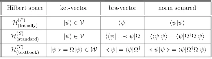
Table 2. 3HS notation: A given stateψin three alternative representations.
Hilbert space ket-vector bra-vector norm squared
H((friendly)F) |ψi ∈ V hψ| hψ|ψi
H((standard)S) |ψi ∈ V hhψ|=≺ψ|Ω hhψ|ψi=hψ|Ω†Ω|ψi H((textbook)T) |ψ≻= Ω|ψi ∈ W ≺ψ|=hψ|Ω† ≺ψ|ψ≻=hψ|Ω†Ω|ψi
3.2 Metric-eliminating transformation Ω
The explicit use of mappings between Hilbert spaces is quite common in textbooks [3] where aunitarymap (e.g., Fourier transformation Ω) produces the correspondence. In the 3HS context the same transition is being postulated,
|ψi ∈ H(F,S) =⇒ |ψ≻≡Ω|ψi ∈ H(T). (5)
Nevertheless, the majority of the nontrivial aspects of the present three-Hilbert-space approach to quantum models will only emerge when Ω ceases to be norm-preserving (let us still say unitary). In such a setting the two physical spaces of states H(S) and H(T) are accompanied by their unphysical partner H(F). This partnership can already be perceived as aiming at a reformulation of quantum theory. Another hint lies in the isospectrality of the Hamiltonians, of which h acts in H(T) while H ≡Ω−1hΩ acts in H(F) or in H(S). This opens a constructive possibility of the choice of a Hamiltonian which isallowedto be non-Hermitian (cf. equation (1)). In nuce, our present main technical trick is that in place of the unitary transformation of spaces (4) (i.e., the second option in equation (5)) we intend to achieve the same goal indirectly, by means of the technically less difficult and non-unitary transition between the other two Hilbert spaces [i.e., via the first option in equation (5)],
H(auxiliary)(Dirac)
=H(F)
→ H(standard)(Dirac)
=H(T)
both of which are equipped with the same and, namely, trivial Dirac metric. The key features of the latter idea may be read out of the parallelled Tables 1and 2.
A detailed inspection of Table2reveals the coincidence of the kets in the “F” and “S” doublet. The mapping between the respective “S” and “T” Hilbert spaces H(S) and H(T) preserves the
inner product and is, in this sense, unitary,
≺ψ′|ψ≻=hhψ′|ψi.
Equivalent physical predictions will be obtained in bothof the latter spaces. The third pair of the “Dirac-metric” spaces with Θ(Dirac) =I and superscripts “F” and “T” shares the form of the Hermitian conjugation.
Table2 can be arranged, as vector spaces, in the following triangular ket-vector pattern
In parallel we have to study the bras. After the transition to the conjugate vector spaces of functionals the above-indicated pattern gets modified as follows,
dual vector spaceW′
In the second row of Table 1 one finds the condition of the Hermiticity of our Hamiltonian h
inH(T). The pullback of this condition toH(F) gives
H†= ΘHΘ−1, Θ = Ω†Ω = Θ†>0 (6)
so that our upper-case Hamiltonian is similar to its Hermitian conjugate or, in the terminology of [7,8], it is quasi-Hermitian.
One of the most elementary illustrative examples of a quasi-HermitianH has been proposed by Mostafazadeh [20]. In a toy space H(F) which is just two-dimensional, this Hamiltonian is represented by the two-dimensional matrix
city (6) can be read as four linear homogeneous algebraic equations determining the matrix elements of all the eligible positive definite matrices Θ = Θ(AM). The general solution of these equations
Any other observable quantity must be represented by the operator Λ which is also quasi-Hermitian with respect to the same metric,
ΘΛ = Λ†Θ. (9)
In this family of solutions the range of the four real parameters a,p,q and dis only restricted by the inequality (a−d)2 >4pqwhich guarantees the reality of both the observable eigenvalues
and by the single nontrivial constraint resulting from quasi-Hermiticity equation,
p=qr2+ (a−d)rcosZ. (11)
Once we fixZ andf >0 in equation (8), an illustrative factorization ΘZ = Ω†ZΩZ of the metric can be performed, say, in terms of triangular matrices,
ΩZ =
This definition specifies, finally, the family of eligible selfadjoint Z-dependent Hamiltonians
h(AM)∼hZ=
cosZ eiβsinZ e−iβsinZ −cosZ
defined by pullback to H(T) and isospectral withH(AM). The same pullback mapping must be
also applied to the second observable Λ of course.
Marginally, let us mention that in many items of the current literature (well exemplified by [11]) the factorization of Θ is only being made in terms of very special Hermitian and positive definite mapping operators Ω(herm)= Θ1/2. In this context our illustrative example shows that
the choice of the special Ω(herm) is just an arbitrary decision rather than a necessity dictated by the mathematical framework of quantum theory. We shall see below that a consistent treatment of the ambiguity of our choice of Ω is in fact very similar to the treatment of the ambiguity encountered [7] during the assignment of the metric Θ to a given Hamiltonian H.
5
Covariant construction of the generator of time-evolution
In the 3HS formulation of quantum physics we may start building phenomenological models inside any item of the triplet H(F,S,T). Still, in a way noticed in [20] and worked out in [9] this freedom may be lost when one decides to admit also the models where the parameters which define the system and its properties (i.e., say, the parameters in the quasi-Hermitian HamiltonianH of equation (7) and/or in another observable Λ given by equation (10)) become allowed to vary with time. Typically, this time-dependence may involve not only the external forces which control the system but also, in principle, the related measuring equipment.
In such an overall setting one has to imagine that the constraints imposed upon the assignment of a suitable metric Θ, say, to a given H and Λ may prove impossible. In the language of our illustrative example this danger has been illustrated in [20] where in illustrative example (7) the so called quasistationarity condition Θ 6= Θ(t) has been shown to imply that r 6=r(t) and
β 6=β(t). The mathematical reason was easy to find since the quasi-stationary time-dependent generalization of the set of constraints (6) and (9) proved overcomplete.
5.1 Time-dependence and Schr¨odinger equations
In [9] we have shown the reasons why the same overrestrictive role is played by the overcomplete-ness also in the generic, model-independent quasi-stationary scenario. In the opposite direction, our study [9] recommended to relax the quasi-stationarity constraint as too artificial. Then, the 3HS formalism proved applicable in its full strength. Now, we intend to show that it restricts the form of the time-dependence of the operators of observables as weakly as possible.
exceptional space H(T) which offers the absence of all doubts in the physical interpretation of any 3HS model. In particular, the time-evolution will be controlled by the textbook Schr¨odinger equation in H(T),
i∂t|ψ(t)≻=h|ψ(t)≻.
This is fully compatible with the textbook concepts of the measurement [3] based on the idea that the complete physical information about a given system prepared in the so called pure state is compressed in its time-dependent wave function |ψ(t)≻.
Secondly, inH(T)there are also no doubts about the standard postulate that all of the other
measurable characteristics of the system in question are obtainable as eigenvalues or mean values of the other operators of observables exemplified here, for the sake of simplicity, byλ= ΩΛΩ−1.
The analysis of this aspect of the problem is postponed to the next section here.
5.2 Models with time-dependent Hamiltonians
In a preparatory step of the study of the time-evolution problem let us just be interested in the single observable (viz., Hamiltonian) and let us admit that a manifest time-dependence occurs in all of the operators,
h(t) = Ω(t)H(t)Ω−1(t).
An easier part of our task is to write the time-dependent Schr¨odinger equation inH(T),
i∂t|ϕ(t)≻=h(t)|ϕ(t)≻.
Its formal solution |ϕ(t)≻=u(t)|ϕ(0)≻employs just the usual evolution operator,
i∂tu(t) =h(t)u(t) (12)
which is unitary inH(T) so that we can conclude that the norm of the state in question remains
constant,
≺ϕ(t)|ϕ(t)≻=≺ϕ(0)|ϕ(0)≻.
In the next step we recollect all our previous considerations and define |ϕ(t)i= Ω−1(t)|ϕ(t) ≻
and hhϕ(t)| =≺ ϕ(t)|Ω(t). We are then able to distinguish between the two formal evolution rules in the physical spaceH(S). One of them controls the evolution of kets,
|ϕ(t)i=UR(t)|ϕ(0)i, UR(t) = Ω−1(t)u(t)Ω(0)
while the other one (written here in its H(F)-space conjugate form) applies to ketkets |·ii ≡ (hh·|)†,
|ϕ(t)ii=UL†(t)|ϕ(0)ii, UL†(t) = Ω†(t)u(t)
Ω−1(0)†
.
The pertaining differential operator equations for the two (viz., right and left) evolution opera-tors read
i∂tUR(t) =−Ω−1(t) [i∂tΩ(t)]UR(t) +H(t)UR(t)
and
i∂tUL†(t) =H†(t)U † L(t) +
i∂tΩ†(t)
Ω−1(t)†
respectively. They are obtained, very easily, by the elementary insertions of the definitions. Inside H(S), the conservation of the norm hhϕ(t)|ϕ(t)i of states is re-established and paralleled
by the same phenomenon inside H(T). One has to solve, therefore, the two equations which form the doublet of non-Hermitian partners of the standard single evolution equation (12) in the third and most computation-friendly space H(F).
We may conclude that the conservation of the norm of the states which evolve with time inH(S)becomes a trivial consequence of the unitary equivalence of the model to its image inH(T) (cf. the explicit formulae in Table 1). One can also recommend the abbreviation ˙Ω(t) ≡∂tΩ(t) which enables us to introduce the time-evolution generator inH(F),
H(gen)(t) =H(t)−iΩ−1(t) ˙Ω(t).
Its most remarkable feature is that it remains the same forboththe time-dependent Schr¨odinger equations in H(S),
i∂t|Φ(t)i=H(gen)(t)|Φ(t)i, (13)
i∂t|Φ(t)ii=H(gen)(t)|Φ(t)ii. (14)
A virtually equally remarkable feature of the operatorH(gen)(t) is that itceasesto be an
elemen-tary observable inH(S)[21]. This is very natural of course. The reason is that by our assumption
the time-dependence of the system ceases to be generated solely by the Hamiltonian (i.e., energy-operator). Indeed, the manifest time-dependence of the other operators of observables represents an independent and equally relevant piece of input information about the dynamics.
6
The two-by-two example revisited
The core of our present message is that after the change of the representation of the Hilbert space of states H(T) → H(S) one should not insist on the survival of the time-dependent Schr¨odinger equation in its usual form where the Hamiltonian acts as the generator of time shift. We have shown that the doublet of equations (13) + (14) must be used instead. Such a replacement opens the space for the consistent use of a broad class of metrics (i.e., spaces H(S)) which vary with time!
The consequences of the new freedom in Θ = Θ(t) may be illustrated again on our elementary two-by-two model (7) where both the parameters r = r(t) ∈ R\ {0} and β = β(t) ∈ R may
nowarbitrarilydepend on time. In such an exemplification the explicit time-dependence of the metric
Θ(t) =f(t)·ΘZ(t), ΘZ(t)=
1 r(t)eiβ(t)cosZ(t)
r(t)e−iβ(t)cosZ(t) r2(t)
appears to havetwoindependent sources. Firstly it results from the direct transfer of the mani-fest time-dependence from the Hamiltonian H(t). Secondly, a new source of time-dependence enters via the new free function Z(t) of time. Obviously, its time-dependence may be read either as responsible for the time-dependence freedom in the metric Θ(t) or as a consequence of the time-dependence of the second observable Λ(t) which is, in principle, independently pre-scribed.
For the first time the latter connection between metric Θ(t) and observables H(t) and Λ(t) has been noticed by the authors of [22] and formulated in [20]. One can conclude that in similar situations we are not allowed to impose additional conditions upon Θ(t) so that the inner products in our Hilbert spaceH(S) vary with time in general.
This looks like a paradox but its essence is sufficiently clearly illustrated by our example where, due to its simplicity, all the one-to-one correspondence between the variations of ob-servables and the metric is mediated by the mere single function Z(t). The time-dependence of Z(t) enters the game via an external specification of some particular form of the observ-able Λ(t). Nevertheless, we already know that this observable must have the above-mentioned four-parametric structure (10). Its four real parametersa(t),p(t),q(t) andd(t)must bemutually coupled by the time-dependent version of constraint (11),
p(t) =q(t)r2(t) + [a(t)−d(t)]r(t) cosZ(t).
This formula may easily be reinterpreted as an implicit def inition of the originally arbitrary function,
Z(t) = arccos p(t)−q(t)r
2(t)
[a(t)−ad(t)]r(t).
In our illustrative two-by-two example we may conclude that the input information about the time-dependence of Λ(t) represents and independent and relevant contribution to the time-dependence of the metric. Thus, even if we just parallel the construction of Section 4 and employ the triangular factorization of the metric with,
ΩZ(t)=
1 r(t)eiβ(t)cosZ(t)
0 r(t) sinZ(t)
the difference between the two operators H(t) and H(gen)(t) (representable by a slightly cum-bersome closed formula) will not vanish in general.
7
Summary
The main message of this text is a confirmation of the full compatibility of several recent applications of quantum theory with its standard form known to us from textbooks. This being said, the present innovative 3HS formulation of the theory can be classified as lying very close, in its spirit if not dictum, to the one offered by Scholtz et al. [7]. Here we just showed that there is no need to feel afraid of the use (i) of the 3HS-extended Dirac notation and (ii) of the concept of covariance in the applications of the theory to the systems where observables happen to be manifestly time-dependent.
In the literature, depending on the respective authors, the applications in question carry the respective names of quasi-Hermitian quantum mechanics (cf. the oldest two proposals offered, practically independently, in mathematics [8] and physics [7]), PT-symmetric quantum mecha-nics (= the best advertised Carl Bender’s trademark [6]), pseudo-Hermitian quantum mechamecha-nics (= perceivably more general concept dating back to M.G. Krein and given second life by Ali Mostafazadeh [15], with possible applications reaching far beyond quantum mechanics) or cryp-tohermitian quantum mechanics (by my opinion, the most explanatory name proposed, only very recently, by Andrei Smilga).
between these two ingredients in phenomenology were probably Bender and Wu [23]. Almost forty years ago they discovered that for the quartic anharmonic oscillator of coupling g > 0 all the spectrum of bound state energies E0(g) < E1(g) < · · · is given by the single analytic
functionof complexg.
Although this amazingly close correspondence between the analytic and LA aspects of bound states still eludes a full appreciation, its other manifestation has been revealed by Bender and Boettcher ten years ago [2]. They conjectured that for a family of elementary and analytic com-plexoscillator potentialsallthe spectrum of bound state energies E0< E1<· · · isstrictly real.
Three years later, the purely analytic aspects have been shown decisive in a rigorous proof of the reality of the spectrum [24]. One year later, several consequences have been drawn also in a 2HS reformulation of the underlying LA formalism of quantum theory [14]. Anad hocoperator of metric Θ =CP has been introduced there. In LA language, as a indirect consequence of the analyticity of the Bender’s and Boettcher’s potentials, two non-equivalent Hilbert spaces, i.e., in our present notation,H(F,S) proved needed.
A counterintuitive limitation of the 2HS formalism to the models with time-independent met-rics Θ6= Θ(t) has been revealed by A. Mostafazadeh [20]. In [9] we removed this limitation via an introduction of the third Hilbert space (in our present notation, ofH(T)). Unfortunately, we preserved the Mostafazadeh’s 2HS notation which made the resulting gem of the 3HS formalism clumsy.
In our present paper we introduced, therefore, an adequate generalization of the traditional Dirac notation and described the updated 3HS formulation of quantum theory in full detail. We also illustrated this formalism via an elementary solvable two-dimensional matrix example. This example demonstrates some details of the theory and of its applications. In particular, the solvability of this example underlines an easy nature of the transition to the models with time-dependent metric.
In the summary we would like to emphasize that the use of the triplet of Hilbert spaces H(F,S,T) and of the related adapted Dirac notation can find its applicability in many apparently
different contexts ranging from computational and variational nuclear physics [7] and analytic perturbation theory [25] through phenomenological field theory [6] up to the first quantization of Klein–Gordon field [11] or Proca’s field [13]. For the nearest future one could therefore encourage the use of the time-dependent metric Θ(t) in all of these physically interesting con-texts.
A
The standard Dirac notation and its shortcomings
In some elementary introductions to Quantum Mechanics the abstract concept of Hilbert spaceH is being replaced by its concrete representations, say, ℓ2 where the elements of the space are
identified with the ordered sets of complex numbers arranged as column vectors. To each of these elements one then associates a dual row vector obtained via the so called Hermitian-conjugation operation (i.e., transposition plus complex Hermitian-conjugation). Similarly, the analysis of some concrete physical quantum systems can be based on the restriction of our attention to the other concrete representations of H like, e.g., the functional space L2(R) as mentioned
in Section 1 or the Klein–Gordon-equation space H(auxiliary) = L2(R)LL2
(R) as cited at the
beginning of Section 2.
One of the most serious weaknesses of such a pedagogically simplified approach is that when-ever we start analyzing the quasi-Hermitian models with property (1) we are forced to turn attention to a modified inner product [7]. This means that in order to avoid confusion one has to replace the concrete models like ℓ2 by the more general notion of the abstract Hilbert space
A.1 Dif f iculties with variable inner products
The term “Hilbert space” and its symbol Hcan be assigned the precise mathematical meaning in several ways. One of the most common definitions specifies the abstract Hilbert spaceH as a vector space V = VH equipped with a suitable inner product. By this “product” a complex number c ∈C is assigned to any pair of elementsa and b of V. In the Dirac-inspired notation
many authors write simplyc=ha|bi (cf., e.g., [15]).
The main advantage of such a von Neumann-inspired approach is that it does not require the knowledge of the more general concept of Banach spaces and that it still enables us to overcome certain mathematical difficulties in rigorous manner. The most serious ones emerge when the vector spaceV ceases to be finite-dimensional. Then, the abstract inner-product spaces of this type are required complete as metric spaces. A dual partnerV′ of the vector spaceV itself is also very easily defined, in this language, as a set of bounded linear maps µ:V →C. Furthermore,
the requirement of the self-duality of Hilbert spaceHcan be reformulated as the existence of a (by far not unique) isomorphism T between vector spaces V and V′. The “canonical” isomorphism T(Dirac) :a→ µ(Dirac)a witha∈ V is usually introduced by the formula µ(Dirac)a (·) =ha|·i, i.e., it clearly and explicitly depends on our choice of the initial inner producth·|·i.
Whenever we decide to work with the single and fixed inner producth·|·i, we are allowed to identify the elements a of V with the Dirac’s ket-vectors |ai. The parallel identification of the linear functionalsµ(Dirac)b (·)∈ V′with the Dirac’s bra-vectorshb|remains equally straightforward but it will not survive a change of the inner product. This is an important observation. Whenever we follow Bender and Boettcher [2] and turn our attention to a quasi-Hermitian quantum model we are forced to endow the given,singlevector spaceV withtwodifferent inner products. Some authors [15] characterize the second, modified inner product by its double bracketing,hh·|·ii. The price to be paid for this rather unfortunate decision is that the consistent use of the unmodified Dirac’s notation ceases to be possible.
A.2 Mostafazadeh’s [15] single-Hilbert-space notation conventions
It is not too easy to find an appropriate notation when a given phenomenological Hamiltonian is quasi-Hermitian, i.e., manifestly non-Hermitian in the sense of equation (1). The main difficulty is that in order to get the states properly normalized, one has to move from the initial, naive Hilbert spaceH(auxiliary) to the physically correct H(standard).
In similar situations, one often feels afraid of using the Dirac’s notation or its analogs3. In practice, such a loss of contact between the Hermitian and quasi-Hermitian observables would be rather unpleasant. For this reason people often try to preserve at least part of this nota-tion. Mostafazadeh [15] offers one of the latter, modified notation conventions which became rather popular in the related literature. Let us briefly recollect some of its principles and rules, therefore.
First of all we have to imagine that the violation of the Hermiticity of a given HamiltonianH
inH(auxiliary)implies that the eigenstates ofHand of its conjugateH†(as defined inH(auxiliary))
will be different in general. This observation has led to the recipe of [15] where one constructs the two independent series of the respective eigenstates4 pertaining tothe sameenergy eigenva-luesEn. These states (numbered byn= 0,1, . . .) must be denoted by twodif ferentsymbols (say, by the “reserved” respective Greek letters Φnand Ψn) when interpreted as ket- and bra-vectors inH(standard),
hΦ|= (|Φi)†∈
H(auxiliary)′
, hΨ|:=hΦ|Θ = (|Φi)‡∈
H(standard)′
.
3This is a wide-spread opinion, especially among mathematicians. 4I.e., two series of ket-vector elements of thesamevector spaceV
Although we are not going to use such a convention here, we summarize it, for our readers, in Table3. We should emphasize that as long as we do not stay within the single Hilbert space H of states, two differentdefinitions of the operation of the Hermitian conjugation emerged in our considerations.
Table 3. 1HS notation of [15] which isnotto be used here.
inner product elements of V their duals their norms HamiltoniansH
h·|·i (inH(auxiliary)) |Φi hΦ|= (|Φi)† hΦ|Φi “pseudo-Hermitian” hh·|·ii(in H(standard)) |Φi hΨ|= (|Φi)‡ hΨ|Φi “quasi-Hermitian”
We see that even without switching to the full-fledged 2HS or 3HS language5, one must keep trace of the change of the inner product via an appropriate modification of the notation. In this manner one formally re-establishes the rigorous meaning of the necessary Hermiticity of the Hamiltonian in the updated, second, physical Hilbert space,
H =H‡ in H(standard).
As we already mentioned, the so called metric operator (denoted by symbol Θ here) can be also used in order to make the underlying definitions less implicit,
O‡≡Θ−1O†Θ.
In this manner one establishes the new, generalized, Θ-dependent Hermitian conjugation oper-ation which applies to any operatorO acting in H(standard).
B
A few remarks on the simplif ied Dirac notation
in both the 2HS and 3HS approaches
As long as the dual-vector definition is inner-product dependent, the very operation of the (generalized) Hermitian conjugation is metric-dependent. We recommend that the single-cross superscript†stays reserved for its use inH(auxiliary)where Θ =I and that it becomes paralleled
by its double-cross analogue ‡ inH(standard) where Θ6=I.
B.1 Metric operator Θ and the 2HS language
A change of the inner product does not necessarily require asimultaneouschangeha|bi → hha|bii of boththe Dirac’s bra and ket graphical symbols. This point of view will be advocated in what follows. Although, formally, its formulation could start from the idea of selfduality and be made equally rigorous as in the approach presented in the preceding two subsections, we shall skip the details here.
Some of the practical merits of such an approach have been discussed and advocated, e.g., in the study [16] of quantum knots. An even less formal notation convention has been shown working in one of the oldest papers on the subject of quasi-Hermiticity [7]. There one finds no double brackets and only the so called metric operator Θ appears there6 as a key to the transition (2) between Hilbert spaces.
5I.e., not speaking openly about the two or threedifferentHilbert spacesH.
Even in the 1HS language, the temporary return to Table3and the updatehha|bii −→ ha|Θ|bi of the graphical representation of the lower inner product seems fairly well suited for empha-sizing the inner-product dependence of the canonical linear functionals. Although such a 1HS convention seems insufficient in more complicated models, its 2HS amendment of [9] proved already sophisticated enough to clarify the emergence of Θ6=I and to render it interpreted as an introduction of a newdual spaceV(non-Dirac)′ withmodifiedelements (i.e., functionals)
µ(non-Dirac)b (·) =hΘb|·i.
This version of the 2HS approach can be complemented by the proposal of a more compact notation as presented, say, in [16]. In essence, one just abbreviatesµ(non-Dirac)b (·)−→ hhb|·i.
B.2 A few details of the transition to the 3HS picture
Let us assume that the operators of observables Λ0,Λ1, . . . are admitted non-Hermitian and
that, via a certain non-unitary map Ω, the naive, ill-chosen Hilbert space H(auxiliary)is replaced by another, physical Hilbert spaceH(standard)where the usual probabilistic interpretation of the system in question is being restored. At this point, we shall require that each one of the two roles of H(auxiliary) will be carried by a separate Hilbert space. The first incarnation of H(auxiliary) will be denoted by the symbolH(F). It will keep playing the auxiliary role of a mathematically friendly space without any immediate physical contents. The second, unitarily nonequivalent space will be treated as the truly physical Hilbert space H(T) which is, by assumption, neither mathematically easily accessible nor user-friendly in the context of physics. Its only comparative advantage will be assumed to lie in a return to the simplicity of the metric, Θ(T)=I.
After such an absolutely minimal extension of the current Dirac conventions we may now demand that the third Hilbert spaceH(T) is built over a new, independent vector space W 6=V with the elementsato be marked by the specific, say, spiked version of the Dirac’s kets,a→ |a≻. The dual space forms again a vector spaceW′ with elements b=≺b|. As long as, by definition, Hilbert spaces are self-dual the two vector spaces W andW′ must be isomorphic7.
B.2.1 Marking the coexistence of two conjugations
The two Hilbert spaces H(F,S) were defined here over the same vector space of kets|ψi. In the
most common applications this means that all of these kets may be treated as linear superpo-sitions of the right eigenkets |ni of thesame upper-case Hamiltonian H. As mentioned above, the difference between H(F) and H(S) only emerges during the introduction of the dual space
of functionals. In the former case the elements of the dual space are defined by the “standard” (i.e., Dirac’s) Hermitian conjugation. In the language of the so called PT-symmetric quantum mechanics [6] this definition is provided by an antilinear operator T = T(F) from the vector
space H(F) in its dual space H(F)′
. It transforms each ket-vector into the “usual” bra-vector, T(F):|ψi −→ hψ|, |ψi ∈ H(F). (15) Inside the second Hilbert spaceH(S), in contrast, anotherantilinear operationT =T(S) defines thedifferentHermitian-conjugation operation. At this point one must pay an enhanced attention to the notation, underlying the necessity of a cleardistinction between the “old” (i.e., current, Dirac’s) Hermitian conjugation (15) employed inside the first Hilbert spaceH(F)and the entirely new, very nonstandard conjugation T(S) which is activated inside the second Hilbert space,
T(S): |ψi −→ hhψ|, |ψi ∈ H(S). (16) 7Without any loss of generality we may work again with the canonical form of the isomorphism denoted, say,
by the symbolT(T)
and meaning, in the Dirac’s notation, thatT(T)
In the other words, one is strongly recommended to consult a standard textbook [3] and treat “brabras” hhψ|literally aslinear functionals inH(S).
An easy guide to the acceptance of the alternative, non-Dirac conjugation (16) appears when we notice that in contrast to the Dirac’s inner productha|bibetween|ai ∈ H(F)and|bi ∈ H(F)),
the new Hilbert space H(S) simply allows us to use the new, perceivably less usual, non-Dirac inner productha|Θ|bi between its elements|ai ∈ H(S) and |bi ∈ H(S). Of course, in our present notation we have
hhψ1|ψ2i ≡ hψ1|Θ|ψ2i.
This means that while working inH(S) the explicit remarks concerning the nontrivial metric Θ are redundant. They must only be made when, for some reason, we must or wish to turn our explicit attention to the former Hilbert space H(F).
B.2.2 Simplifying spectral formulae
Besides the most usual spectral formula representing, say, the Hamiltonian in H(T),
h= ∞
X
n=0
|n≻En≺n|
a perceivably more complicated relation emerges for its isospectral partner which is an operator inH(F) orH(S),
H =
∞
X
n=0
Ω−1|n≻En≺n|Ω. (17)
Together with the natural innovation of the basis kets in H(F,S),
|ni:= Ω−1|n≻
we may also introduce another set of “ketket” vectors in both these spaces,
|nii:= Ω†|n≻≡Ω†Ω|ni ≡Θ|ni ∈ H(F,S).
Formula (17) then acquires a particularly compact form inH(S),
H =
∞
X
n=0
|niEnhhn|
and an explicitly metric-dependent form inH(F),
H =
∞
X
n=0
|niEnhn|Θ.
In the same spirit we may deduce that
≺m|n≻=δm,n =hhm|ni=hm|Θ|ni, m, n= 0,1, . . . .
B.2.3 Making use of the maps between spaces
Let us now change and broaden the perspective used during our discussion of the illustrative example in Section 4 and assume that we start from the knowledge of the lower-case Hamil-tonian h acting in physical H(T) and from the choice of an arbitrary orthogonal basis in H(S)
composed of its brabras hhm| and kets|mi which are connected by conjugation (16). Without any loss of generality we may further use some suitable unitary transformations and represent our mapping operator in a simplified single-series form
Ω = ∞
X
n=0
|n≻µnhhn|.
Allµn∈C\ {0}areindependentfree parameters. By insertion we may immediately verify that these variable parameters enter also the metric operator,
Θ = Ω†Ω≡ ∞
X
n=0
|niiµ∗nµnhhn|.
This operator [7,17] must be Hermitian, positive definite and invertible, i.e., the operators
Ω−1 =
must be assumed to exist. Under this assumption one could have an impression that, in principle at least, we might be able to get rid of the use of the rather exotic concepts of the non-Hermitian Hamiltonians and/or of the biorthogonal bases in H(F). In practice, this impression proves wrong. In the majority of applications as reviewed in [6] one virtually always works solely insideH(F)employing both the other two spacesH(T,S)as purely auxiliary theoretical constructs. Nevertheless, one should keep in mind that whenever we try to complement the results of our calculations by their correct probabilistic interpretation, theexplicituse of the two-step mapping
H(F)→ H(S) → H(T)
proves unavoidable.
Acknowledgements
In various stages of development the work has been supported by Institutional Research Plan AV0Z10480505, by the MˇSMT “Doppler Institute” project Nr. LC06002, by GA ˇCR, grant Nr. 202/07/1307 and by the hospitality of Universidad de Santiago de Chile. Last but not least, three anonymous referees should be acknowledged for their constructive commentaries.
References
[1] Styer D.F. et al., Nine formulations of quantum mechanics,Amer. J. Phys.70(2002), 288–297.
[2] Bender C.M., Boettcher S., Real spectra in non-Hermitian Hamiltonians havingP T symmetry,Phys. Rev. Lett.80(1998), 5243–5246,physics/9712001.
Bender C.M., Boettcher S., Meisinger P.M.,P T-symmetric quantum mechanics,J. Math. Phys.40(1999),
2201–2229,quant-ph/9809072.
[3] Messiah A., Quantum mechanics, North Holland, Amsterdam, 1961, Vols. 1, 2.
[5] Proceedings of the Workshop “Pseudo-Hermitian Hamiltonians in Quantum Physics” (Prague, June 2003), Editor M. Znojil,Czech. J. Phys.54(2004), no. 1.
Proceedings of the Workshop “Pseudo-Hermitian Hamiltonians in Quantum Physics II” (Prague, June 2004), Editor M. Znojil,Czech. J. Phys.54(2004), no. 10.
Proceedings of the Workshop “Pseudo-Hermitian Hamiltonians in Quantum Physics III” (Istanbul, June 2005), Editor M. Znojil,Czech. J. Phys.55(2005), no. 9.
Proceedings of the Workshop “Pseudo-Hermitian Hamiltonians in Quantum Physics IV” (Stellenbosch, November 2005), Editors H. Geyer, D. Heiss and M. Znojil,J. Phys. A: Math. Gen.39(2006), no. 32.
Proceedings of the Workshop “Pseudo-Hermitian Hamiltonians in Quantum Physics V” (Bologna, July 2006), Editor M. Znojil,Czech. J. Phys.56(2006), no. 9.
Proceedings of the Workshop “Pseudo-Hermitian Hamiltonians in Quantum Physics VI” (London, July 2007), Editors by A. Fring, H. Jones and M. Znojil,J. Phys. A: Math. Theor.41(2008), no. 24.
Proceedings of the Workshop “Pseudo-Hermitian Hamiltonians in Quantum Physics VII” (Benasque, July 2008), Editors A. Andrianov et al.,SIGMA5(2009).
[6] Bender C.M., Making sense of non-Hermitian Hamiltonians, Rep. Progr. Phys. 70 (2007), 947–1018, hep-th/0703096.
[7] Scholtz F.G., Geyer H.B., Hahne F.J.W., Quasi-Hermitian operators in quantum mechanics and the varia-tional principle,Ann. Physics213(1992), 74–101.
[8] Dieudonne J., Quasi-Hermitian operators, in Proc. Internat. Sympos. Linear Spaces (Jerusalem, 1960), Pergamon, Oxford, 1961, 115–122.
Williams J.P., Operators similar to their adjoints,Proc. Amer. Math. Soc.20(1969), 121–123.
[9] Znojil M., Time-dependent version of cryptohermitian quantum theory, Phys. Rev. D 78(2008), 085003,
5 pages,arXiv:0809.2874.
[10] Bender C.M., Turbiner A., Analytic continuation of eigenvalue problems, Phys. Lett. A 173(1993), 442–
446.
G¨unther U., Stefani F., Znojil M., MHD α2-dynamo, squire equation and P T-symmetric interpolation between square well and harmonic oscillator,J. Math. Phys.46(2005), 063504, 22 pages,math-ph/0501069.
Jakubsk´y V., Thermodynamics of pseudo-Hermitian systems in equilibrium,Modern Phys. Lett. A22(2007),
1075–1084,quant-ph/0703092.
Mostafazadeh A., Loran F., Propagation of electromagnetic waves in linear media and pseudo-Hermiticity,
Europhys. Lett. EPL81(2008), 10007, 6 pages,physics/0703080.
[11] Mostafazadeh A., Hilbert space structures on the solution space of Klein–Gordon type evolution equations,
Classical Quantum Gravity20(2003), 155–172,math-ph/0209014.
[12] Feshbach H., Villars F., Elementary relativistic wave mechanics of spin 0 and spin 1/2 particles,Rev. Mod. Phys.30(1958), 24–45.
[13] Jakubsk´y V., Smejkal J., A positive-definite scalar product for free proca particle,Czech. J. Phys.56(2006),
985–997,hep-th/0610290.
Smejkal J., Jakubsk´y V., Znojil M., Relativistic vector bosons andP T-symmetry,J. Phys. Stud.11(2007),
45–54,hep-th/0611287.
Zamani F., Mostafazadeh A., Quantum mechanics of Proca fields,arXiv:0805.1651.
[14] Bender C.M., Brody D.C., Jones H.F., Complex extension of quantum mechanics, Phys. Rev. Lett. 89
(2002), 270402, 4 pages, Erratum,Phys. Rev. Lett.92(2004), 119902,quant-ph/0208076.
[15] Mostafazadeh A., Pseudo-Hermiticity versus P T symmetry: the necessary condition for the reality of the spectrum of a non-Hermitian Hamiltonian,J. Math. Phys.43(2002), 205–214,math-ph/0107001.
Mostafazadeh A., Pseudo-hermiticity versusP T-symmetry. II. A complete characterization of non-Hermitian Hamiltonians with a real spectrum,J. Math. Phys.43(2002), 2814–2816,math-ph/0110016.
Mostafazadeh A., Pseudo-Hermitian quantum mechanics,arXiv:0810.5643.
[16] Znojil M., Quantum knots,Phys. Lett. A372(2008), 3591–3596,arXiv:0802.1318.
Znojil M., Identification of observables in quantum toboggans,J. Phys. A: Math. Theor.41(2008), 215304,
14 pages,arXiv:0803.0403.
[17] Znojil M., On the role of the normalization factorsκnand of the pseudo-metricP 6=P†in crypto-Hermitian
quantum models,SIGMA4(2008), 001, 9 pages,arXiv:0710.4432.
[18] Cannata F., Dedonder J.-P., Ventura A., Scattering in P T-symmetric quantum mechanics, Ann. Physics 322(2007), 397–433,quant-ph/0606129.
Znojil M., Scattering theory with localized non-Hermiticites, Phys. Rev. D 78 (2008), 025026, arXiv:0805.2800.
Znojil M., DiscreteP T-symmetric models of scattering,J. Phys. A: Math. Theor.41(2008), 292002, 9 pages, arXiv:0806.2019.
[20] Mostafazadeh A., Time-dependent pseudo-Hermitian Hamiltonians defining a unitary quantum system and uniqueness of the metric,Phys. Lett. B650(2007), 208–212,arXiv:0706.1872.
[21] Znojil M., Which operator generates time evolution in quantum mechanics?,arXiv:0711.0535.
[22] Figueira de Morisson Faria C., Fring A., Time evolution of non-Hermitian Hamiltonian systems,J. Phys. A: Math. Gen.39(2006), 9269–9289,quant-ph/0604014.
[23] Bender C.M., Wu T.T., Anharmonic oscillator,Phys. Rev.184(1969), 1231–1260.
[24] Sibuya Y., Global theory of second order linear differential equation with polynomial coefficient, North Holland, Amsterdam, 1975.
Dorey P., Dunning C., Tateo R., Spectral equivalences, Bethe ansatz equations, and reality properties in
P T-symmetric quantum mechanics,J. Phys. A: Math. Gen.34(2001), 5679–5704,hep-th/0103051.
Dorey P., Dunning C., Tateo R., Supersymmetry and the spontaneous breakdown of P T symmetry,
J. Phys. A: Math. Gen.34(2001), L391–L400,hep-th/0104119.
Dorey P., Dunning C., Tateo R., The ODE/IM correspondence,J. Phys. A: Math. Theor.40(2007), R205–
R283,hep-th/0703066.
Davies E.B., Linear operators and their spectra, Cambridge, Cambridge University Press, 2007.
[25] Caliceti E., Graffi S., Maioli M., Perturbation theory of odd anharmonic oscillators,Comm. Math. Phys. 75(1980), 51–66.
Buslaev V., Grecchi V., Equivalence of unstable anharmonic oscillators and double wells,J. Phys. A: Math. Gen.26(1993), 5541–5549.
![Table 3. 1HS notation of [15] which is not to be used here.](https://thumb-ap.123doks.com/thumbv2/123dok/910423.900048/14.612.88.538.144.222/table-hs-notation-used.webp)
