ELECTRONIC
COMMUNICATIONS in PROBABILITY
RANDOM WALKS THAT AVOID THEIR
PAST CONVEX HULL
OMER ANGEL
Dept. of Mathematics, Weizmann Institute of Science, Rehovot 76100, Israel email: [email protected]
ITAI BENJAMINI
Dept. of Mathematics, Weizmann Institute of Science, Rehovot 76100, Israel (Research partially supported by the Israeli Science Foundation)
email: [email protected]
B ´ALINT VIR ´AG
Dept. of Mathematics, MIT, Cambridge, MA 02139, USA (Research partially supported by NSF grant #DMS-0206781) email: [email protected]
Submitted December 9, 2001, accepted in final form January 29, 2003 AMS 2000 Subject classification: 60K35. Secondary: 60G50, 52A22, 91B28 Keywords: self-avoiding walk, random walk, convex sets
Abstract
We explore planar random walk conditioned to avoid its past convex hull. We prove that it escapes at a positive lim sup speed. Experimental results show that fluctuations from a limiting direction are on the order of n3/4. This behavior is also observed for the extremal investor, a natural financial model related to the planar walk.
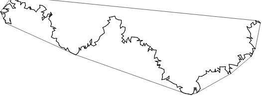
Figure 1: 300 steps of the rancher
1
Introduction
Consider the following walk in Rd. Letx0 = 0, and given the pastx0, . . . , xn letxn+1 to be uniformly distributed on the sphere of radius 1 around xn but conditioned so that the step
segmentxnxn+1does not intersect the interior of the convex hull of{x0, . . . , xn}. We will call
this process therancher’s walkor simply the rancher.
The name comes form the planar case: a frontier rancher who is walking about and at each step increases his ranch by dragging with him the fence that defines it, so that the ranch at any time is the convex hull of the path traced until that time. This paper studies the planar case of the process.
Since the model provides some sort of “repulsion” of the rancher from his past, it can be expected that the rancher will escape faster than a regular random walk. In fact, he has positive lim sup speed.
Theorem 1 There exists a constants >0 such thatlim supkxnk/n≥sa.s.
Simulations suggest that in factkxnk/n converges a.s. to some fixeds≈0.314.
In Section 2 we discuss simulations of the model. In particular, we consider how far is the ranch after n steps from a straight line segment. The experiments suggest that the farthest point in the path from the lineoxn connecting its end-points is at a distance of ordern3/4.
In Section 3 we discuss a related one-dimensional model that we call theextremal investor. This models the fluctuations in a stock’s price, when it is subject to market forces that depend on the stock’s best and worst past performance in a certain simple way. As a result, the relation between the stock’s history and its drift is similar to the same relation for the rancher. Simulations for the critical case of this process yield the same exponent 3/4, distinguishing it from one-dimensional Brownian motion where the exponent equals 1/2.
The rancher’s walk falls into the large category of self-interacting random walks, such as rein-forced, self-avoiding, or self-repelling walks. These models are difficult to analyze in general. The reader should consult [1], [2], [6], [4], and especially the survey papers [5], [3] for examples.
2
Simulations: scaling limit and the exponent 3/4
Unlike the self-avoiding walk, the rancher is not difficult to simulate in nearly linear time. At any given time we only need to keep track of the convex hull of the random walk’s trace so far. If the points on the boundary of the convex hull are kept in cyclic order, updating the convex hull is a matter of finding the largest and smallest elements in a cyclic array, which is monotone on each of the two arcs connecting the extreme values.
With at mostnpoint on the hull, one can update it in order logntime, giving a running time of ordernlognfornsteps of the walk. In fact, the number of points defining the convex hull is much smaller thann, and the extremal elements tend to be very close in the array to the previous point of the walk. This and the actual running times suggest that the theoretical running time is close to linear.
3.5 4 4.5 5 5.5 6 log steps 1.5
2.5 3 3.5 4 log width
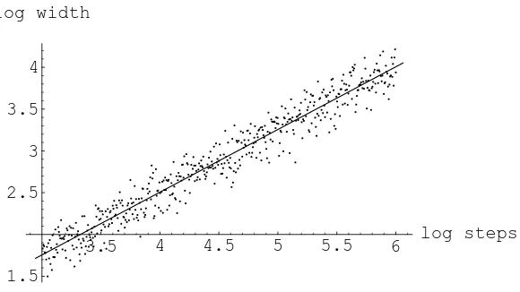
Figure 3: The dimensions of the ranch
In our simulations kxnk/n appears to converge to some fixed s ≈ 0.314. Assuming this is
the case, the rancher’s walk is similar to the random walk in the plane conditioned to always increase its distance from the origin. Since the distance is linear innand the step size is fixed, the angular change is of order n−1. If the signs of the angular change were independent this would imply the following.
Conjecture 1 (Angular convergence) The processxn/||xn|| converges a.s.
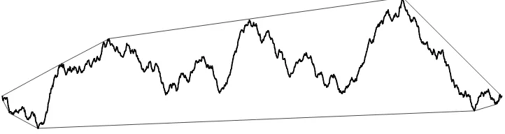
The difficulty in our case is that the angular movements are positively correlated: if a step has a positive angular component, then subsequent steps have a drift in the same direction. Our simulations suggest that these correlations are not strong enough to prevent angular convergence, and we conjecture that this is in fact the case. This is observed in Figure 2, showing a million-step sample of the rancher’s walk. Still larger simulations yield a picture indistinguishable from a straight line segment.
The scaled path of the rancher’s walk appears to converge to a straight line segment, and it is natural to ask how quickly this happens. If we assume positive speed and angular convergence, then each step has a component in the eventual (say horizontal) direction and a component in the perpendicular (vertical) direction.
If the vertical components were independent, the vertical movement would essentially be a simple one-dimensional random walk. Since the horizontal component increase linearly, the path is then roughly the graph of a one-dimensional random walk.
To test this, we measured a related quantity, the width wn of the path at timen, defined as
the distance of the farthest point on the path from the lineoxn. Under the above assumptions,
one would guess thatwn should behave as the maximum up to timenof the absolute value of
a one-dimensional random walk with bounded steps, and have a typical value of ordern1/2. Our simulations, however, show an entirely different picture. Figure 3 is a log base 10 plot of 500 realizations of wn on independent processes. n ranges from a thousand to a million
steps equally spaced on the log scale. The slope of the regression line is 0.746 (SE 0.008). A regression line on the medians of 1000 measurements of walks of length 103,104,105,106gave a value of .75002 (SE 0.002). Based on these simulations, we conjecture that wn behaves like
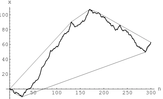
Figure 4: The rancher’s path of Figure 2 rescaled vertically
Conjecture 2 (The exponent 3/4) For everyε >0, asn→ ∞ we have P[n3/4−ε< w
n< n3/4+ε]→1.
It is also feasible that if the path is scaled by a factor ofn3/4in the vertical axis and bynin the horizontal axis (parallel to the segmentoxn) then the law of the path would converge to
some random function. The result of such asymmetric scaling is seen in Figure 4. In the next section we introduce a model that appears closely related.
3
The extremal investor
Stock or portfolio prices are often modeled by exponentiated random walk or Brownian motion. In the simplest discrete-time model, the log stock price, denotedxn, changes every time by an
independent standard Gaussian random variable.
Ones decision whether to invest in, say, a mutual fund is often based on past performance of the fund. Mutual fund companies report past performance for periods ending at present; the periods are often hand-picked to show the best possible performance. The simplest such statistic is the overall best performance over periods ending in the present. In terms of log interest rate it is given by
rnmax= maxm<n
xn−xm
n−m , (1)
that is the maximal slope of lines intersecting the graph of xn in both a past point and the
present point.
A more cautious investor also looks at the worst performance rmin
n , given by (1) with a min,
and makes a decision to buy, sell or hold accordingly, influencing the fund price. In the simplest model, which we call the extremal investor model, the change in the log fund price given the present is simply a Gaussian with standard deviation 1 and expected value given by a fixed influence parameterαtimes the average ofrmax andrmin:
xn+1=xn+α
rmax
n +rminn
2 + standard Gaussian.
This process is related to the rancher in two dimensions, since the future behavior of xn is
influenced through the shape of the convex hull of the graph of xn at the tip. For α= 1 the
50 100 150 200 250 300n 20
40 60 80 100 x
Figure 5: The extremal investor process forα= 1 and its convex hull
Let wn denote the greatest distance between xn and the linear interpolation from time zero
to the present (assume x0= 0):
wn = max m≤n
¯ ¯ ¯xm−
m nxn
¯ ¯ ¯.
The following analogue of Conjecture 2 is consistent with our simulations:
Conjecture 3 (The exponent 3/4 for the extremal investor) Let α = 1. For every ε >0 asn→ ∞ we have
P[n3/4−ε< w
n< n3/4+ε]→1.
A moment of thought shows that for α >1, xn will blow up exponentially, so αc = 1 is the
critical parameter. Forα <1 the behavior ofwnseems to be governed by an exponent between
1/2 and 3/4 depending onα. Forα <1 thexn/nseems to converge to 0, but in the case that
α= 1, it appears thatxn/nconverges a.s. to a random limit.
4
Proof of Theorem 1
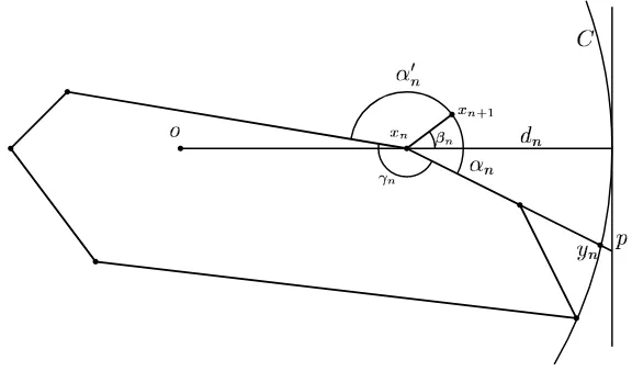
Denote{xn;n≥0}the rancher’s walk. Define theranchRnas the convex hull of{x0, . . . , xn}.
Sincexn is always on the boundary andRnis convex, the angle ofRnatxn is always in [0, π].
Denote this angle byγn (as in Figure 6).
The idea of the proof is to find a set of times of positive upper density in which the expected gain in distance is bounded away from 0. There are two cases where the expected gain in distance can be small. First, if γn is close to 0, the distribution of the next step is close to
uniform on the unit circle. Second, whenγn is close toπ, the next step is uniformly distributed
on roughly a semicircle. If in addition the direction to the origin is near one of the end-points of the semicircle then the expected gain in distance is small.
We now introduce further notation used in the proof. Setsn =kxn+1k−kxnk. Note that since
✁✄✂ ✁✆☎✂
✝✟✞
✝
✞✡✠☞☛
✌ ✞
✍
✞ ✎
✂
✏☞✂✒✑
✓
Figure 6: Notation used in the proof
angleoxnxn+1−πis denoted byβn, so thatβn∈[−π, π). Thusβ= 0 means that the walker
moved directly away fromo,β >0 means that the walker moved counterclockwise.
Let C be the boundary of the smallest closed disk centered at o containing the ranch Rn.
Consider the half-line starting fromxnthat contains the edge ofRnincident to and clockwise
from xn. Let yn denote the intersection of this half line and C. Let αn denote the angle
π−oxnyn, and letα′n denote the analogous angle in the counterclockwise direction. Letdn
be the distance betweenC and xn. It follows from these definitions thatαn+α′n+γn = 2π
and thatβn has uniform distribution on [−αn, α′n].
Proof of Theorem 1. We find a set of times of positive upper density in which Esn is
positive and bounded away from 0. Ifγn ∈[ε, π−ε], thenEsnis bounded from below by some
function ofε. Thus we need only consider the times whenγn < εor whenγn > π−ε, where
ε >0 will be chosen later to satisfy further constraints.
In the case γn < ε, the rancher is at the tip of a thin ranch, so a single step can make a
large change inγ, thus we look at two consecutive steps. With probability at least a quarter βn ∈[π/4,3π/4]. In that case γn+1 is bounded away from both 0 andπ, and then Esn+1 is bounded away from 0. If βn is not in [π/4,3π/4], we use the boundEsn+1 >0. Combining these gives a uniform positive lower bound onEsn+1.
Ifγnis close toπ, then we are in a tighter spot: it could stay large for several steps, andEsn
may remain small. The rest of the proof consists of showing that at a positive fraction of time the angleγn is not close toπ.
Ifdn < D, whereDis some large bound to be determined later, then with probability at least
half γn+1< π−1/(2D), thus if we take ε≤1/(2D), it suffices to show that a.s. the Markov process{(Rn, xn)}returns to the setA={(R, x)|d < D}at a set of times with positive upper
density.
To show this, we use a martingale argument; it suffices to exhibit a functionf(Rn, xn) bounded
from below, so that the expected increase inf given the present is negative and bounded away from zero when (Rn, xn)6∈A, and is bounded from above when (Rn, xn)∈A. The sufficiency
of the above is proved in Lemma 1 below; there take An to be the event (Rn, xn)∈A, and
The standard function that has this property is the expected hitting time of A. We will try to guess this. The motivation for our guess is the following heuristic picture. When the angle α is small, it has a tendency to increase by a quantity of order roughly 1/d, and d tends to decrease by a quantity of orderα. This means thatdperforms a random walk with downward drift at least 1/d, but this is not enough for positive recurrence. So we have to wait for a few steps forαto increase enough to provide sufficient drift ford; the catch is that in every step αhas a chance of orderαto decrease, and the same order of chance to decrease to a fraction of its size. So αtends to grow steadily and collapse suddenly. If the typical size isα∗, then it takes order 1/α∗ time to collapse. During this time it grows by about 1/(dα∗), which should be on the order of the typical sizeα∗, givingα∗=d−1/2. This suggests that the processdhas drift of this order, so the expected hitting time of 0 is of order d3/2. A more accurate guess takes into account the fact that ifαis large, the hitting time is smaller.
Define the functionsf1(d) =d3/2, andf2(d, α) =−((cd1/2)∧(αd)), where is a constant to be
First we consider the expected change in f1. All expected values will be conditional on the information available at time n. To simplify notation, assume xn is on the positive X-axis.
This may be done since the process is invariant to rotations of the plane. We first bound the expected decrease dn−dn+1.
where here (and later)o(1) denotes a quantity that is arbitrarily small ifDis taken sufficiently large (D will be fixed later so that these term is small enough).
We now proceed to bound the expected change inf2(dn, αn); denote this change by ∆f2. We
break up ∆f2 into important and unimportant parts:
∆f2 = (cd1n/2∧αndn−cd1n/2∧αn+1dn)
+ (cd1n/2∧αn+1dn−cd1n/+12 ∧αn+1dn)
The second term is bounded above byc|d1n/+12 −d 1/2
n |=o(1). The third term is non-positive
un-lesscd1n/+12 > αn+1dn, implying thatαn+1< cd −1/2
n , and then this term is at mostαn+1|∆d|= o(1). Thus important increase can only come from the first term. We therefore denote
z= (cd1n/2∧αndn−cd1n/2∧αn+1dn),
and consider three cases given by the following events, which depend on the value ofβ =βn:
B1={β∈[−αn,0)}, B2={β ∈[0, π−αn]}, B3={β∈(π−αn, α′n]}.
As we will see in detail, the contribution of the first and last cases is small. If αn is small
enough then the second also has a small contribution, while ifαnis large the negative expected
change off1offsets any positive change inf2.
EventB2:β ∈[0, π−αn] (equivalently,xn+1is on the side opposite ofRnfor the linesoxnand
xnyn). In this case the rancher moves sufficiently away from the ranch, so thatαincreases:
∆α = oxnyn−oxn+1yn+1≥oxnyn−oxn+1yn
= xnoxn+1+xn+1ynxn≥xn+1ynxn≥0. (4)
All inequalities follow from our assumption B2. The equality follows from the fact that the angles in the quadrangleoxnynxn+1 add up to 2π.
We now compute the last angle in (4) using a simple identity in the trianglexnynxn+1, and
the value of the angleynxnxn+1:
kxn+1−ynksin(xn+1ynxn) =kxn−xn+1ksin(ynxnxn+1) = sin(βn+αn). (5)
A byproduct of (4) is thatB2impliesz≤0. Ifαn< cd−n1/2/2, then a better bound is possible:
kxn+1−ynk ≤1 +kxn−ynk ≤1 +kxn−pk= 1 +dn(cosαn)−1=dn(1 +o(1)),
where the pointpis the intersection of the line xnyn and the tangent toC perpendicular to
Event B1: β <0. We can boundαn+1 below byβ+αn as follows. First, note that αn+1= π−oxn+1yn+1≥π−oxn+1yn. Alsoβ+αn =ynxnxn+1=π−xnxn+1yn−xn+1ynxn, since
the angles of a triangle add toπ. We can splitxnxn+1yn=xnxn+1o+oxn+1yn. Putting these
together we get αn+1 = β+αn+xnxn+1o+xn+1ynxn, and since the latter two angles are
small and positive, αn+1> β+αn. Therefore
P[0< zandB1]≤P[β+αn< cdn−1/2]≤cd−n1/2π−1,
and as in case B3:
E[z; B1]≤c2/π.
Summarizing the casesB1, B2, B3 we get the bound
E∆f2(d, α)≤2c2π−1+o(1),
and ifα < cd−1/2/2, then
E∆f2(d, α)≤2c2π−1
−2π−1+o(1).
Of course, the same bounds hold for f2(d, α′).
We now summarize our estimates on all the components of ∆f.
• Ifαn < cd−1/2/2, then
E∆f = E∆f1+E∆f2(d, α) +E∆f2(d, α′)
≤ 0 + (2c2−2)π−1+ 2c2π−1+o(1) = 4c2−2
π +o(1),
which is negative for largeD ifc <2−1/2. The same bound holds ifα′
n< cd−1/2/2.
• If at least one ofαn, α′n is in [cd−1/2/2, π−cd
−1/2
n /2], then using (3), we get
E∆f ≤ −3/8π−1c+o(1) + 4c2π−1+o(1) =4c
2−3c/8
π +o(1),
which is negative for largeD ifc <3/32.
• Ifαn, α′n > π−cd
−1/2
n /2, anddn > Dis large enough, then we have seen that the two
step driftEdn+2−dn<−c1for somec1>0. Thus in this caseE∆f1≤ −c1d1n/2+o(1),
while the drift off2is uniformly bounded.
Putting the three cases together shows that if we take 0< c <3/32 then for large enoughD the function f satisfies the requirements of Lemma 1.
For the following technical lemma, we use the notation ∆man=an+m−an, and ∆an= ∆1an.
Lemma 1 Let{(Xn, fn, An)}be a sequence of triples adapted to the increasing filtration{Fn}
There exist positive constantsc1, c2, c3, c4, and a positive integerm, so we have a.s. for all n
|∆Xn| ≤ 1,
E[∆Xn | Fn] ≥ 0, (7)
E[∆mXn | Fn, An] > c1, (8)
fn > −c2,
∆fn1(An) < c3, (9)
E[∆fn | Fn, Acn] < −c4. (10)
Then for some positive constantc5 we have
lim supXn/n > c5 a.s. (11)
Proof. LetGn =Pn−1
i=0 1Ai, and let Gn,k =
Pn−1
i=0 1Ami+k, 0 ≤k < n. First we show that
them+ 1 processes
{c1Gn,k−Xmn+k}n≥0, 0≤k < m, (12)
{fn−c3Gn+c4(n−Gn)}n≥0 (13)
are supermartingales adapted to {Fmn+k}n≥0, 0 ≤ k < m, {Fn}n≥0, respectively. For the firstmprocesses fixk, and note thatE[c1(Gn+1,k−Gn,k)|Fmn+k] =c11(Amn+k). Consider
E[c1(Gn+1,k−Gn,k)| Fmn+k] +E[−(Xm(n+1)+k−Xmn+k)| Fmn+k]
If Amn+k happens, then the first term equals c1, and the second is less than −c1 by (8). If
Amn+k does not happen, then the first term equals 0 and the second is non-positive by (7).
Putting these two together shows that (12) are supermartingales. For the last process, consider
E[∆fn| Fn] +E[−c3∆Gn| Fn] +E[c4(1−∆Gn)| Fn].
If An happens, then the first term is less than c3 by (9), the second term equals −c3, and
the last equals 0. If An does not happen, then the first term is less than −c4 by (10), the
second term equals 0, and the third equalsc4. In both cases we get that the process (13) is a supermartingale.
It follows from the supermartingale property that for somec >0 and all n≥0 we have
EXmn+k ≥ c1EGn,k−c, 0≤k < m, (14)
EGn ≥ c4/(c3+c4)n−c. (15)
Since Gmn =Gn,0+. . .+Gn,m−1, it follows from (15) that for some c6 >0 and all large n there is k =k(n), so that EGn,k > c6n. Then for some c7 >0 we have EXnm+k > c7n by
(14). As a consequence, forYn= max{Xmn, . . . , Xmn+m−1}we have EYn> c7n.
Thus for somec8 <1 we haveE(1−Yn/(mn))< c8 for all largen. Since Xn ≤X0+n, we
haveYn≤X0+mn+m−1 =mn+c9 and therefore 1−(Yn−c9)/(mn)≥0. Fatou’s lemma
then implies
Elim inf(1−Yn/(mn)) =Elim inf(1−(Yn−c9)/(mn))≤c8,
for somec10∈(c8,1) Markov’s inequality givesP(lim inf(1−Yn/(mn))< c8/c10)>1−c10.
So for somec5>0,
but we can repeat this argument while conditioning on theσ-fieldFtto get
P(lim supXn/n > c5 | Ft)>1−c10
so lettingt→ ∞by L´evy’s 0-1 law we get (11).
5
Further open questions and conjectures
Conjecture 4 Theorem 1 holds withlim inf instead oflim sup.
Conjecture 5 The speedlimkxnk/n exists and is constant a.s. This could follow from some
super-linearity result on the rancher’s travels.
Question 6 What is the scaling limit of the asymmetrically normalized path?
Question 7 What is the behavior in higher dimensions? Is the lim sup (or even lim inf ) speed still positive? If not, iskxnk=O(√n)or is it significantly faster then a simple random walk?
What about convergence of direction?
Question 8 If longer step sizes are allowed what happens when the tail is thickened? Are there distributions which give positive speed without convergence of direction?
Acknowledgments. The authors thank the anonymous referees for their helpful comments on previous versions of this paper.
References
[1] B. Davis, Reinforced random walk. Probab. Theory Related Fields 84 (1990), no. 2, 203–229.
[2] G. Lawler, Intersections of random walks. Probability and its Applications. Birkh¨auser Boston, Inc., Boston, MA, 1991.
[3] R. Pemantle, Random processes with reinforcement. Preprint.
http://www.math.ohio-state.edu/~pemantle/papers/Papers.html
[4] O. Schramm, Scaling limits of loop-erased random walks and uniform spanning trees. Israel J. Math.118 (2000), 221–288.
[5] B. T´oth, Self-interacting random motions – a survey.In: Random walks – A Collection of Surveys.Eds: P. R´ev´esz and B. T´oth.Bolyai Society Mathematical Studies, vol. 9., Budapest, 1998.