MATLAB
®
7
www.mathworks.com/contact_TS.html
[email protected] Product enhancement suggestions
[email protected] Bug reports
[email protected] Documentation error reports
[email protected] Order status, license renewals, passcodes
[email protected] Sales, pricing, and general information
508-647-7000 (Phone)
508-647-7001 (Fax)
The MathWorks, Inc.
3 Apple Hill Drive
Natick, MA 01760-2098
For contact information about worldwide offices, see the MathWorks Web site.
MATLAB®Getting Started Guide
© COPYRIGHT 1984–2010 by The MathWorks, Inc.
The software described in this document is furnished under a license agreement. The software may be used or copied only under the terms of the license agreement. No part of this manual may be photocopied or reproduced in any form without prior written consent from The MathWorks, Inc.
FEDERAL ACQUISITION: This provision applies to all acquisitions of the Program and Documentation by, for, or through the federal government of the United States. By accepting delivery of the Program or Documentation, the government hereby agrees that this software or documentation qualifies as commercial computer software or commercial computer software documentation as such terms are used or defined in FAR 12.212, DFARS Part 227.72, and DFARS 252.227-7014. Accordingly, the terms and conditions of this Agreement and only those rights specified in this Agreement, shall pertain to and govern the use, modification, reproduction, release, performance, display, and disclosure of the Program and Documentation by the federal government (or other entity acquiring for or through the federal government) and shall supersede any conflicting contractual terms or conditions. If this License fails to meet the government’s needs or is inconsistent in any respect with federal procurement law, the government agrees to return the Program and Documentation, unused, to The MathWorks, Inc.
Trademarks
MATLAB and Simulink are registered trademarks of The MathWorks, Inc. See
www.mathworks.com/trademarksfor a list of additional trademarks. Other product or brand names may be trademarks or registered trademarks of their respective holders.
Patents
MathWorks products are protected by one or more U.S. patents. Please see
Revision History
December 1996 First printing For MATLAB 5 May 1997 Second printing For MATLAB 5.1 September 1998 Third printing For MATLAB 5.3
September 2000 Fourth printing Revised for MATLAB 6 (Release 12) June 2001 Online only Revised for MATLAB 6.1 (Release 12.1) July 2002 Online only Revised for MATLAB 6.5 (Release 13) August 2002 Fifth printing Revised for MATLAB 6.5
Contents
Getting Started
Introduction
1
Product Overview
. . . .
1-2Overview of the MATLAB Environment
. . . .
1-2The MATLAB System
. . . .
1-3Documentation
. . . .
1-5Starting and Quitting the MATLAB Program
. . . .
1-7Starting a MATLAB Session
. . . .
1-7Quitting the MATLAB Program
. . . .
1-8Matrices and Arrays
2
Matrices and Magic Squares
. . . .
2-2About Matrices
. . . .
2-2Entering Matrices
. . . .
2-4sum, transpose, and diag
. . . .
2-5Subscripts
. . . .
2-7The Colon Operator
. . . .
2-8The magic Function
. . . .
2-9Expressions
. . . .
2-11Variables
. . . .
2-11Numbers
. . . .
2-12Generating Matrices
. . . .
2-17The load Function
. . . .
2-18Saving Code to a File
. . . .
2-18Concatenation
. . . .
2-19Deleting Rows and Columns
. . . .
2-20More About Matrices and Arrays
. . . .
2-21Linear Algebra
. . . .
2-21Arrays
. . . .
2-25Multivariate Data
. . . .
2-27Scalar Expansion
. . . .
2-28Logical Subscripting
. . . .
2-28The find Function
. . . .
2-29Controlling Command Window Input and Output
. . . .
2-31The format Function
. . . .
2-31Suppressing Output
. . . .
2-32Entering Long Statements
. . . .
2-33Command Line Editing
. . . .
2-33Graphics
3
Overview of Plotting
. . . .
3-2Plotting Process
. . . .
3-2 [image:6.558.139.457.43.520.2]Graph Components
. . . .
3-6Figure Tools
. . . .
3-7Arranging Graphs Within a Figure
. . . .
3-14Choosing a Type of Graph to Plot
. . . .
3-15Editing Plots
. . . .
3-23Plot Edit Mode
. . . .
3-23Some Ways to Use Plotting Tools
. . . .
3-29Plotting Two Variables with Plotting Tools
. . . .
3-29Changing the Appearance of Lines and Markers
. . . .
3-32Adding More Data to the Graph
. . . .
3-33Changing the Type of Graph
. . . .
3-36Modifying the Graph Data Source
. . . .
3-38Preparing Graphs for Presentation
. . . .
3-43Annotating Graphs for Presentation
. . . .
3-43Printing the Graph
. . . .
3-48Exporting the Graph
. . . .
3-52Using Basic Plotting Functions
. . . .
3-56Creating a Plot
. . . .
3-56Plotting Multiple Data Sets in One Graph
. . . .
3-57Specifying Line Styles and Colors
. . . .
3-58Plotting Lines and Markers
. . . .
3-59Graphing Imaginary and Complex Data
. . . .
3-61Adding Plots to an Existing Graph
. . . .
3-62Figure Windows
. . . .
3-63Displaying Multiple Plots in One Figure
. . . .
3-64Controlling the Axes
. . . .
3-66Adding Axis Labels and Titles
. . . .
3-67Saving Figures
. . . .
3-68Creating Mesh and Surface Plots
. . . .
3-72About Mesh and Surface Plots
. . . .
3-72Visualizing Functions of Two Variables
. . . .
3-72Plotting Image Data
. . . .
3-80About Plotting Image Data
. . . .
3-80Reading and Writing Images
. . . .
3-81Printing Graphics
. . . .
3-82Overview of Printing
. . . .
3-82Printing from the File Menu
. . . .
3-82Exporting the Figure to a Graphics File
. . . .
3-83Using the Print Command
. . . .
3-83Understanding Handle Graphics Objects
. . . .
3-85Programming
4
Flow Control
. . . .
4-2Conditional Control — if, else, switch
. . . .
4-2Loop Control — for, while, continue, break
. . . .
4-5Error Control — try, catch
. . . .
4-7Program Termination — return
. . . .
4-8Other Data Structures
. . . .
4-9Multidimensional Arrays
. . . .
4-9Cell Arrays
. . . .
4-11Characters and Text
. . . .
4-13Structures
. . . .
4-16Scripts and Functions
. . . .
4-20Overview
. . . .
4-20Scripts
. . . .
4-21Functions
. . . .
4-22Types of Functions
. . . .
4-24Global Variables
. . . .
4-26Passing String Arguments to Functions
. . . .
4-27The eval Function
. . . .
4-28Function Handles
. . . .
4-28Function Functions
. . . .
4-29Vectorization
. . . .
4-31Preallocation
. . . .
4-32Object-Oriented Programming
. . . .
4-33MATLAB Classes and Objects
. . . .
4-33Data Analysis
5
Introduction
. . . .
5-2Preprocessing Data
. . . .
5-3Overview
. . . .
5-3Loading the Data
. . . .
5-3Missing Data
. . . .
5-3Outliers
. . . .
5-4Smoothing and Filtering
. . . .
5-6Summarizing Data
. . . .
5-10Overview
. . . .
5-10Measures of Location
. . . .
5-10Measures of Scale
. . . .
5-11Shape of a Distribution
. . . .
5-11Visualizing Data
. . . .
5-14Overview
. . . .
5-142-D Scatter Plots
. . . .
5-143-D Scatter Plots
. . . .
5-16Scatter Plot Arrays
. . . .
5-18Exploring Data in Graphs
. . . .
5-19Modeling Data
. . . .
5-27Overview
. . . .
5-27Polynomial Regression
. . . .
5-27General Linear Regression
. . . .
5-28Creating Graphical User Interfaces
6
What Is GUIDE?
. . . .
6-2Laying Out a GUI
. . . .
6-3Desktop Tools and Development Environment
7
Desktop Overview
. . . .
7-2Introduction to the Desktop
. . . .
7-2Arranging the Desktop
. . . .
7-3Start Button
. . . .
7-3Command Window and Command History
. . . .
7-5Command Window
. . . .
7-5Command History
. . . .
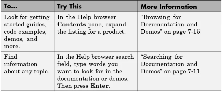
7-6Getting Help
. . . .
7-7Ways to Get Help
. . . .
7-7Accessing Documentation, Examples, and Demos Using the Help Browser
. . . .
7-9Searching for Documentation and Demos
. . . .
7-11Browsing for Documentation and Demos
. . . .
7-15Running Demos and Code in Examples
. . . .
7-16Workspace Browser and Variable Editor
. . . .
7-20Workspace Browser
. . . .
7-20Variable Editor
. . . .
7-21Managing Files in MATLAB
. . . .
7-23How MATLAB Helps You Manage Files
. . . .
7-23Making Files Accessible to MATLAB
. . . .
7-23Using the Current Folder Browser to Manage Files
. . . .
7-24More Ways to Manage Files
. . . .
7-26Finding and Getting Files Created by Other Users —
Editor
. . . .
7-29Editing MATLAB Code Files
. . . .
7-29Identifying Problems and Areas for Improvement
. . . .
7-31Publishing MATLAB Code Files
. . . .
7-34Improving and Tuning Your MATLAB Programs
. . . . .
7-38Finding Errors Using the Code Analyzer Report
. . . .
7-38Improving Performance Using the Profiler
. . . .
7-40External Interfaces
8
Programming Interfaces
. . . .
8-2Call MATLAB Software from C/C++ and Fortran
Programs
. . . .
8-2Call C/C++ and Fortran Programs from MATLAB Command Line
. . . .
8-2Call Sun Java Commands from MATLAB Command
Line
. . . .
8-3Call Functions in Shared Libraries
. . . .
8-3Import and Export Data
. . . .
8-3Interface to .NET Framework
. . . .
8-4Component Object Model Interface
. . . .
8-5Web Services
. . . .
8-6Serial Port Interface
. . . .
8-7_
Getting Started
The MATLAB®high-performance language for technical computing integrates
computation, visualization, and programming in an easy-to-use environment where problems and solutions are expressed in familiar mathematical notation. You can watch the Getting Started with MATLAB video demo for an overview of the major functionality. If you have an active Internet connection, you can also watch the Working in the Development Environment video demo, and the Writing a MATLAB Program video demo. This collection includes the following topics:
Chapter 1, Introduction (p. 1-1) Describes the components of the MATLAB system
Chapter 2, Matrices and Arrays (p. 2-1)
How to use MATLAB to generate matrices and perform mathematical operations on matrices
Chapter 3, Graphics (p. 3-1) How to plot data, annotate graphs, and work with images
Chapter 4, Programming (p. 4-1) How to use MATLAB to create scripts and functions, how to construct and manipulate data structures
Chapter 5, Data Analysis (p. 5-1) How to set up a basic data analysis
Chapter 6, Creating Graphical User Interfaces (p. 6-1)
Introduces GUIDE, the MATLAB graphical user interface development environment.
Chapter 7, Desktop Tools and Development Environment (p. 7-1)
Information about tools and the MATLAB desktop
Chapter 8, External Interfaces (p. 8-1)
1
Introduction
• “Product Overview” on page 1-2
• “Documentation” on page 1-5
Product Overview
In this section...
“Overview of the MATLAB Environment” on page 1-2
“The MATLAB System” on page 1-3
Overview of the MATLAB Environment
MATLAB is a high-level technical computing language and interactive environment for algorithm development, data visualization, data analysis, and numeric computation. Using the MATLAB product, you can solve technical computing problems faster than with traditional programming languages, such as C, C++, and Fortran.
You can use MATLAB in a wide range of applications, including signal and image processing, communications, control design, test and measurement, financial modeling and analysis, and computational biology. Add-on toolboxes (collections of special-purpose MATLAB functions, available separately) extend the MATLAB environment to solve particular classes of problems in these application areas.
MATLAB provides a number of features for documenting and sharing your work. You can integrate your MATLAB code with other languages and applications, and distribute your MATLAB algorithms and applications. Features include:
• High-level language for technical computing
• Development environment for managing code, files, and data
• Interactive tools for iterative exploration, design, and problem solving
• Mathematical functions for linear algebra, statistics, Fourier analysis, filtering, optimization, and numerical integration
• 2-D and 3-D graphics functions for visualizing data
Product Overview
• Functions for integrating MATLAB based algorithms with external applications and languages, such as C, C++, Fortran, Java™, COM, and Microsoft®Excel®
The MATLAB System
The MATLAB system consists of these main parts:
Desktop Tools and Development Environment
This part of MATLAB is the set of tools and facilities that help you use and become more productive with MATLAB functions and files. Many of these tools are graphical user interfaces. It includes: the MATLAB desktop and Command Window, an editor and debugger, a code analyzer, and browsers for viewing help, the workspace, and folders.
Mathematical Function Library
This library is a vast collection of computational algorithms ranging from elementary functions, like sum, sine, cosine, and complex arithmetic, to more sophisticated functions like matrix inverse, matrix eigenvalues, Bessel functions, and fast Fourier transforms.
The Language
The MATLAB language is a high-level matrix/array language with control flow statements, functions, data structures, input/output, and object-oriented programming features. It allows both “programming in the small” to
rapidly create quick programs you do not intend to reuse. You can also do “programming in the large” to create complex application programs intended for reuse.
Graphics
External Interfaces
Documentation
Documentation
The MATLAB program provides extensive documentation, in both printable and HTML format, to help you learn about and use all of its features. If you are a new user, begin with this Getting Started guide. It covers all the primary MATLAB features at a high level, including many examples.
To view the online documentation, selectHelp > Product Helpin MATLAB. Online help appears in the Help browser, providing task-oriented and reference information about MATLAB features. For more information about using the Help browser, see “Getting Help” on page 7-7.
The MATLAB documentation is organized into these main topics:
• Desktop Tools and Development Environment — Startup and shutdown, arranging the desktop, and using tools to become more productive with MATLAB
• Data Import and Export — Retrieving and storing data, memory-mapping, and accessing Internet files
• Mathematics — Mathematical operations
• Data Analysis — Data analysis, including data fitting, Fourier analysis, and time-series tools
• Programming Fundamentals — The MATLAB language and how to develop MATLAB applications
• Object-Oriented Programming — Designing and implementing MATLAB classes
• Graphics — Tools and techniques for plotting, graph annotation, printing, and programming with Handle Graphics®objects
• 3-D Visualization — Visualizing surface and volume data, transparency, and viewing and lighting techniques
• Creating Graphical User Interfaces — GUI-building tools and how to write callback functions
• External Interfaces — MEX-files, the MATLAB engine, and interfacing to Sun Microsystems™ Java software, Microsoft®.NET Framework, COM,
There is reference documentation for all MATLAB functions:
• Function Reference — Lists all MATLAB functions, listed in categories or alphabetically
• Handle Graphics Property Browser — Provides easy access to descriptions of graphics object properties
• C/C++ and Fortran API Reference — Covers functions used by the MATLAB external interfaces, providing information on syntax in the calling language, description, arguments, return values, and examples
The MATLAB online documentation also includes:
• Examples — An index of examples included in the documentation
• Release Notes — New features, compatibility considerations, and bug reports for current and recent previous releases
• Printable Documentation — PDF versions of the documentation, suitable for printing
In addition to the documentation, you can access demos for each product from the Help browser. Run demos to learn about key functionality of MathWorks®
Starting and Quitting the MATLAB®Program
Starting and Quitting the MATLAB Program
In this section...
“Starting a MATLAB Session” on page 1-7
“Quitting the MATLAB Program” on page 1-8
Starting a MATLAB Session
On Microsoft Windows®platforms, start the MATLAB program by
double-clicking the MATLAB shortcut on your Windows desktop.
On Apple Macintosh®platforms, start MATLAB by double-clicking the
MATLAB icon in theApplicationsfolder.
On UNIX®platforms, start MATLAB by typingmatlabat the operating
system prompt.
When you start MATLAB, by default, MATLAB automatically loads all the program files provided by MathWorks for MATLAB and other MathWorks products. You do not have to start each product you want to use.
There are alternative ways to start MATLAB, and you can customize
MATLAB startup. For example, you can change the folder in which MATLAB starts or automatically execute MATLAB statements upon startup.
For More InformationSee “Startup and Shutdown” in the Desktop Tools and Development Environment documentation.
The Desktop
When you start MATLAB, the desktop appears, containing tools (graphical user interfaces) for managing files, variables, and applications associated with MATLAB.
about the desktop tools, see Chapter 7, “Desktop Tools and Development Environment”.
View or change the current folder.
Move, minimize, resize, or close a tool. Enter MATLAB
statements at the prompt.
Menus change, depending on the tool you are using.
Quitting the MATLAB Program
To end your MATLAB session, selectFile > Exit MATLABin the desktop, or typequitin the Command Window. You can run a script file named
Starting and Quitting the MATLAB®Program
Confirm Quitting
MATLAB can display a confirmation dialog box before quitting. To set this option, selectFile > Preferences > General > Confirmation Dialogs, and select the check box forConfirm before exiting MATLAB.
2
Matrices and Arrays
You can watch the Getting Started with MATLAB video demo for an overview of the major functionality.
• “Matrices and Magic Squares” on page 2-2
• “Expressions” on page 2-11
• “Working with Matrices” on page 2-17
• “More About Matrices and Arrays” on page 2-21
Matrices and Magic Squares
In this section...
“About Matrices” on page 2-2
“Entering Matrices” on page 2-4
“sum, transpose, and diag” on page 2-5
“Subscripts” on page 2-7
“The Colon Operator” on page 2-8
“The magic Function” on page 2-9
About Matrices
Matrices and Magic Squares
Entering Matrices
The best way for you to get started with MATLAB is to learn how to handle matrices. Start MATLAB and follow along with each example.
You can enter matrices into MATLAB in several different ways:
• Enter an explicit list of elements.
• Load matrices from external data files.
• Generate matrices using built-in functions.
• Create matrices with your own functions and save them in files.
Start by entering Dürer’s matrix as a list of its elements. You only have to follow a few basic conventions:
• Separate the elements of a row with blanks or commas.
• Use a semicolon,;, to indicate the end of each row.
• Surround the entire list of elements with square brackets,[ ].
To enter Dürer’s matrix, simply type in the Command Window
Matrices and Magic Squares
MATLAB displays the matrix you just entered:
A =
16 3 2 13
5 10 11 8
9 6 7 12
4 15 14 1
This matrix matches the numbers in the engraving. Once you have entered the matrix, it is automatically remembered in the MATLAB workspace. You can refer to it simply asA. Now that you haveAin the workspace, take a look at what makes it so interesting. Why is it magic?
sum, transpose, and diag
You are probably already aware that the special properties of a magic square have to do with the various ways of summing its elements. If you take the sum along any row or column, or along either of the two main diagonals, you will always get the same number. Let us verify that using MATLAB. The first statement to try is
sum(A)
MATLAB replies with
ans =
34 34 34 34
When you do not specify an output variable, MATLAB uses the variableans, short foranswer, to store the results of a calculation. You have computed a row vector containing the sums of the columns ofA. Each of the columns has the same sum, themagicsum, 34.
How about the row sums? MATLAB has a preference for working with the columns of a matrix, so one way to get the row sums is to transpose the matrix, compute the column sums of the transpose, and then transpose the result. For an additional way that avoids the double transpose use the dimension argument for thesumfunction.
diagonal, and also changes the sign of the imaginary component of any complex elements of the matrix. The dot-apostrophe operator (e.g.,A.'), transposes without affecting the sign of complex elements. For matrices containing all real elements, the two operators return the same result.
So
A'
produces
ans =
16 5 9 4
3 10 6 15
2 11 7 14
13 8 12 1
and
sum(A')'
produces a column vector containing the row sums
ans = 34 34 34 34
The sum of the elements on the main diagonal is obtained with thesumand thediagfunctions:
Matrices and Magic Squares and sum(diag(A)) produces ans = 34
The other diagonal, the so-calledantidiagonal,is not so important mathematically, so MATLAB does not have a ready-made function for it. But a function originally intended for use in graphics,fliplr, flips a matrix from left to right:
sum(diag(fliplr(A))) ans =
34
You have verified that the matrix in Dürer’s engraving is indeed a magic square and, in the process, have sampled a few MATLAB matrix operations. The following sections continue to use this matrix to illustrate additional MATLAB capabilities.
Subscripts
The element in rowiand columnjofAis denoted byA(i,j). For example,
A(4,2)is the number in the fourth row and second column. For the magic square,A(4,2)is15. So to compute the sum of the elements in the fourth column ofA, type
A(1,4) + A(2,4) + A(3,4) + A(4,4)
This subscript produces
ans = 34
but is not the most elegant way of summing a single column.
It is also possible to refer to the elements of a matrix with a single subscript,
which case the array is regarded as one long column vector formed from the columns of the original matrix. So, for the magic square,A(8)is another way of referring to the value15stored inA(4,2).
If you try to use the value of an element outside of the matrix, it is an error:
t = A(4,5)
Index exceeds matrix dimensions.
Conversely, if you store a value in an element outside of the matrix, the size increases to accommodate the newcomer:
X = A; X(4,5) = 17
X =
16 3 2 13 0
5 10 11 8 0
9 6 7 12 0
4 15 14 1 17
The Colon Operator
The colon,:, is one of the most important MATLAB operators. It occurs in several different forms. The expression
1:10
is a row vector containing the integers from 1 to 10:
1 2 3 4 5 6 7 8 9 10
To obtain nonunit spacing, specify an increment. For example,
100:-7:50
is
100 93 86 79 72 65 58 51
and
Matrices and Magic Squares
is
0 0.7854 1.5708 2.3562 3.1416
Subscript expressions involving colons refer to portions of a matrix:
A(1:k,j)
is the firstkelements of thejth column ofA. Thus:
sum(A(1:4,4))
computes the sum of the fourth column. However, there is a better way to perform this computation. The colon by itself refers toallthe elements in a row or column of a matrix and the keywordendrefers to thelastrow or column. Thus:
sum(A(:,end))
computes the sum of the elements in the last column ofA:
ans = 34
Why is the magic sum for a 4-by-4 square equal to 34? If the integers from 1 to 16 are sorted into four groups with equal sums, that sum must be
sum(1:16)/4
which, of course, is
ans = 34
The magic Function
B = magic(4) B =
16 2 3 13
5 11 10 8
9 7 6 12
4 14 15 1
This matrix is almost the same as the one in the Dürer engraving and has all the same “magic” properties; the only difference is that the two middle columns are exchanged.
To make thisBinto Dürer’sA, swap the two middle columns:
A = B(:,[1 3 2 4])
This subscript indicates that—for each of the rows of matrixB—reorder the elements in the order 1, 3, 2, 4. It produces:
A =
16 3 2 13
5 10 11 8
9 6 7 12
Expressions
Expressions
In this section...
“Variables” on page 2-11
“Numbers” on page 2-12
“Operators” on page 2-13
“Functions” on page 2-14
“Examples of Expressions” on page 2-15
Variables
Like most other programming languages, the MATLAB language provides mathematicalexpressions, but unlike most programming languages, these expressions involve entire matrices.
MATLAB does not require any type declarations or dimension statements. When MATLAB encounters a new variable name, it automatically creates the variable and allocates the appropriate amount of storage. If the variable already exists, MATLAB changes its contents and, if necessary, allocates new storage. For example,
num_students = 25
creates a 1-by-1 matrix namednum_studentsand stores the value 25 in its single element. To view the matrix assigned to any variable, simply enter the variable name.
Variable names consist of a letter, followed by any number of letters, digits, or underscores. MATLAB is case sensitive; it distinguishes between uppercase and lowercase letters. Aandaarenotthe same variable.
Although variable names can be of any length, MATLAB uses only the first
Ncharacters of the name, (whereNis the number returned by the function
N = namelengthmax N =
63
Thegenvarnamefunction can be useful in creating variable names that are both valid and unique.
Numbers
MATLAB uses conventional decimal notation, with an optional decimal point and leading plus or minus sign, for numbers. Scientific notation uses the lettereto specify a power-of-ten scale factor. Imaginary numbers use eitheri
orjas a suffix. Some examples of legal numbers are
3 -99 0.0001
9.6397238 1.60210e-20 6.02252e23
1i -3.14159j 3e5i
MATLAB stores all numbers internally using thelongformat specified by the IEEE®floating-point standard. Floating-point numbers have a finite
precisionof roughly 16 significant decimal digits and a finiterangeof roughly 10-308to 10+308.
Numbers represented in the double format have a maximum precision of 52 bits. Any double requiring more bits than 52 loses some precision. For example, the following code shows two unequal values to be equal because they are both truncated:
x = 36028797018963968; y = 36028797018963972; x == y
ans = 1
Integers have available precisions of 8-bit, 16-bit, 32-bit, and 64-bit. Storing the same numbers as 64-bit integers preserves precision:
x = uint64(36028797018963968); y = uint64(36028797018963972); x == y
Expressions
0
The section “Avoiding Common Problems with Floating-Point Arithmetic” gives a few of the examples showing how IEEE floating-point arithmetic affects computations in MATLAB. For more examples and information, see Technical Note 1108 — Common Problems with Floating-Point Arithmetic.
MATLAB software stores the real and imaginary parts of a complex number. It handles the magnitude of the parts in different ways depending on the context. For instance, thesortfunction sorts based on magnitude and resolves ties by phase angle.
sort([3+4i, 4+3i]) ans =
4.0000 + 3.0000i 3.0000 + 4.0000i
This is because of the phase angle:
angle(3+4i) ans = 0.9273 angle(4+3i) ans = 0.6435
The “equal to” relational operator==requires both the real and imaginary parts to be equal. The other binary relational operators> <,>=, and<=ignore the imaginary part of the number and consider the real part only.
Operators
Expressions use familiar arithmetic operators and precedence rules.
+ Addition
- Subtraction
* Multiplication
\ Left division (described in “Linear Algebra” in the MATLAB documentation)
^ Power
' Complex conjugate transpose
( ) Specify evaluation order
Functions
MATLAB provides a large number of standard elementary mathematical functions, includingabs,sqrt,exp, andsin. Taking the square root or logarithm of a negative number is not an error; the appropriate complex result is produced automatically. MATLAB also provides many more advanced mathematical functions, including Bessel and gamma functions. Most of these functions accept complex arguments. For a list of the elementary mathematical functions, type
help elfun
For a list of more advanced mathematical and matrix functions, type
help specfun help elmat
Some of the functions, likesqrtandsin, arebuilt in. Built-in functions are part of the MATLAB core so they are very efficient, but the computational details are not readily accessible. Other functions are implemented in the MATLAB programing language, so their computational details are accessible.
There are some differences between built-in functions and other functions. For example, for built-in functions, you cannot see the code. For other functions, you can see the code and even modify it if you want.
Several special functions provide values of useful constants.
pi 3.14159265...
i Imaginary unit,
Expressions
eps Floating-point relative precision,
realmin
Smallest floating-point number,
realmax
Largest floating-point number,
Inf Infinity
NaN Not-a-number
Infinity is generated by dividing a nonzero value by zero, or by evaluating well defined mathematical expressions thatoverflow, i.e., exceedrealmax. Not-a-number is generated by trying to evaluate expressions like0/0or
Inf-Infthat do not have well defined mathematical values.
The function names are not reserved. It is possible to overwrite any of them with a new variable, such as
eps = 1.e-6
and then use that value in subsequent calculations. The original function can be restored with
clear eps
Examples of Expressions
You have already seen several examples of MATLAB expressions. Here are a few more examples, and the resulting values:
rho = (1+sqrt(5))/2 rho =
1.6180
a = abs(3+4i) a =
5
z = sqrt(besselk(4/3,rho-i)) z =
huge = exp(log(realmax)) huge =
1.7977e+308
toobig = pi*huge toobig =
Working with Matrices
Working with Matrices
In this section...
“Generating Matrices” on page 2-17
“The load Function” on page 2-18
“Saving Code to a File” on page 2-18
“Concatenation” on page 2-19
“Deleting Rows and Columns” on page 2-20
Generating Matrices
MATLAB software provides four functions that generate basic matrices.
zeros All zeros
ones All ones
rand Uniformly distributed random elements
randn Normally distributed random elements
Here are some examples:
Z = zeros(2,4) Z =
0 0 0 0
0 0 0 0
F = 5*ones(3,3) F =
5 5 5
5 5 5
5 5 5
N = fix(10*rand(1,10)) N =
R = randn(4,4) R =
0.6353 0.0860 -0.3210 -1.2316 -0.6014 -2.0046 1.2366 1.0556 0.5512 -0.4931 -0.6313 -0.1132 -1.0998 0.4620 -2.3252 0.3792
The load Function
Theloadfunction reads binary files containing matrices generated by earlier MATLAB sessions, or reads text files containing numeric data. The text file should be organized as a rectangular table of numbers, separated by blanks, with one row per line, and an equal number of elements in each row. For example, outside of MATLAB, create a text file containing these four lines:
16.0 3.0 2.0 13.0
5.0 10.0 11.0 8.0
9.0 6.0 7.0 12.0
4.0 15.0 14.0 1.0
Save the file asmagik.datin the current directory. The statement
load magik.dat
reads the file and creates a variable,magik, containing the example matrix.
An easy way to read data into MATLAB from many text or binary formats is to use the Import Wizard.
Saving Code to a File
You can create matrices using text files containing MATLAB code. Use the MATLAB Editor or another text editor to create a file containing the same statements you would type at the MATLAB command line. Save the file under a name that ends in.m.
Working with Matrices
A = [16.0 3.0 2.0 13.0
5.0 10.0 11.0 8.0
9.0 6.0 7.0 12.0
4.0 15.0 14.0 1.0 ];
The statement
magik
reads the file and creates a variable,A, containing the example matrix.
Concatenation
Concatenationis the process of joining small matrices to make bigger ones. In fact, you made your first matrix by concatenating its individual elements. The pair of square brackets,[], is the concatenation operator. For an example, start with the 4-by-4 magic square,A, and form
B = [A A+32; A+48 A+16]
The result is an 8-by-8 matrix, obtained by joining the four submatrices:
B =
16 3 2 13 48 35 34 45
5 10 11 8 37 42 43 40
9 6 7 12 41 38 39 44
4 15 14 1 36 47 46 33
64 51 50 61 32 19 18 29
53 58 59 56 21 26 27 24
57 54 55 60 25 22 23 28
52 63 62 49 20 31 30 17
This matrix is halfway to being another magic square. Its elements are a rearrangement of the integers1:64. Its column sums are the correct value for an 8-by-8 magic square:
sum(B)
ans =
But its row sums,sum(B')', are not all the same. Further manipulation is necessary to make this a valid 8-by-8 magic square.
Deleting Rows and Columns
You can delete rows and columns from a matrix using just a pair of square brackets. Start with
X = A;
Then, to delete the second column ofX, use
X(:,2) = []
This changesXto
X =
16 2 13
5 11 8
9 7 12
4 14 1
If you delete a single element from a matrix, the result is not a matrix anymore. So, expressions like
X(1,2) = []
result in an error. However, using a single subscript deletes a single element, or sequence of elements, and reshapes the remaining elements into a row vector. So
X(2:2:10) = []
results in
X =
More About Matrices and Arrays
More About Matrices and Arrays
In this section...
“Linear Algebra” on page 2-21
“Arrays” on page 2-25
“Multivariate Data” on page 2-27
“Scalar Expansion” on page 2-28
“Logical Subscripting” on page 2-28
“The find Function” on page 2-29
Linear Algebra
Informally, the termsmatrixandarrayare often used interchangeably. More precisely, amatrixis a two-dimensional numeric array that represents a linear transformation. The mathematical operations defined on matrices are the subject of linear algebra.
Dürer’s magic square
A = [16 3 2 13
5 10 11 8
9 6 7 12
4 15 14 1 ]
provides several examples that give a taste of MATLAB matrix operations. You have already seen the matrix transpose,A'. Adding a matrix to its transpose produces asymmetricmatrix:
A + A'
ans =
32 8 11 17
8 20 17 23
11 17 14 26
The multiplication symbol,*, denotes thematrixmultiplication involving inner products between rows and columns. Multiplying the transpose of a matrix by the original matrix also produces a symmetric matrix:
A'*A
ans =
378 212 206 360 212 370 368 206 206 368 370 212 360 206 212 378
The determinant of this particular matrix happens to be zero, indicating that the matrix issingular:
d = det(A)
d = 0
The reduced row echelon form ofAis not the identity:
R = rref(A)
R =
1 0 0 1
0 1 0 -3
0 0 1 3
0 0 0 0
Because the matrix is singular, it does not have an inverse. If you try to compute the inverse with
X = inv(A)
you will get a warning message:
Warning: Matrix is close to singular or badly scaled. Results may be inaccurate. RCOND = 9.796086e-018.
More About Matrices and Arrays
condition estimate, is on the order ofeps, the floating-point relative precision, so the computed inverse is unlikely to be of much use.
The eigenvalues of the magic square are interesting:
e = eig(A)
e =
34.0000 8.0000 0.0000 -8.0000
One of the eigenvalues is zero, which is another consequence of singularity. The largest eigenvalue is 34, the magic sum. That sum results because the vector of all ones is an eigenvector:
v = ones(4,1)
v = 1 1 1 1 A*v ans = 34 34 34 34
When a magic square is scaled by its magic sum,
P = A/34
P =
0.4706 0.0882 0.0588 0.3824 0.1471 0.2941 0.3235 0.2353 0.2647 0.1765 0.2059 0.3529 0.1176 0.4412 0.4118 0.0294
Such matrices represent the transition probabilities in aMarkov process. Repeated powers of the matrix represent repeated steps of the process. For this example, the fifth power
P^5
is
0.2507 0.2495 0.2494 0.2504 0.2497 0.2501 0.2502 0.2500 0.2500 0.2498 0.2499 0.2503 0.2496 0.2506 0.2505 0.2493
This shows that as approaches infinity, all the elements in the th power,
, approach .
Finally, the coefficients in the characteristic polynomial
poly(A)
are
1 -34 -64 2176 0
These coefficients indicate that the characteristic polynomial
is
More About Matrices and Arrays
Arrays
When they are taken away from the world of linear algebra, matrices become two-dimensional numeric arrays. Arithmetic operations on arrays are done element by element. This means that addition and subtraction are the same for arrays and matrices, but that multiplicative operations are different. MATLAB uses a dot, or decimal point, as part of the notation for multiplicative array operations.
The list of operators includes
+ Addition
- Subtraction
.* Element-by-element multiplication
./ Element-by-element division
.\ Element-by-element left division
.^ Element-by-element power
.' Unconjugated array transpose
If the Dürer magic square is multiplied by itself with array multiplication
A.*A
the result is an array containing the squares of the integers from 1 to 16, in an unusual order:
ans =
256 9 4 169
25 100 121 64
81 36 49 144
16 225 196 1
Building Tables
Array operations are useful for building tables. Supposenis the column vector
Then
pows = [n n.^2 2.^n]
builds a table of squares and powers of 2:
pows =
0 0 1
1 1 2
2 4 4
3 9 8
4 16 16
5 25 32
6 36 64
7 49 128
8 64 256
9 81 512
The elementary math functions operate on arrays element by element. So
format short g x = (1:0.1:2)'; logs = [x log10(x)]
builds a table of logarithms.
More About Matrices and Arrays
Multivariate Data
MATLAB uses column-oriented analysis for multivariate statistical data. Each column in a data set represents a variable and each row an observation. The(i,j)th element is theith observation of thejth variable.
As an example, consider a data set with three variables:
• Heart rate
• Weight
• Hours of exercise per week
For five observations, the resulting array might look like
D = [ 72 134 3.2
81 201 3.5
69 156 7.1
82 148 2.4
75 170 1.2 ]
The first row contains the heart rate, weight, and exercise hours for patient 1, the second row contains the data for patient 2, and so on. Now you can apply many MATLAB data analysis functions to this data set. For example, to obtain the mean and standard deviation of each column, use
mu = mean(D), sigma = std(D)
mu =
75.8 161.8 3.48
sigma =
5.6303 25.499 2.2107
For a list of the data analysis functions available in MATLAB, type
help datafun
If you have access to the Statistics Toolbox™ software, type
Scalar Expansion
Matrices and scalars can be combined in several different ways. For example, a scalar is subtracted from a matrix by subtracting it from each element. The average value of the elements in our magic square is 8.5, so
B = A - 8.5
forms a matrix whose column sums are zero:
B =
7.5 -5.5 -6.5 4.5
-3.5 1.5 2.5 -0.5
0.5 -2.5 -1.5 3.5
-4.5 6.5 5.5 -7.5
sum(B)
ans =
0 0 0 0
With scalar expansion, MATLAB assigns a specified scalar to all indices in a range. For example,
B(1:2,2:3) = 0
zeroes out a portion ofB:
B =
7.5 0 0 4.5
-3.5 0 0 -0.5
0.5 -2.5 -1.5 3.5
-4.5 6.5 5.5 -7.5
Logical Subscripting
More About Matrices and Arrays
This kind of subscripting can be done in one step by specifying the logical operation as the subscripting expression. Suppose you have the following set of data:
x = [2.1 1.7 1.6 1.5 NaN 1.9 1.8 1.5 5.1 1.8 1.4 2.2 1.6 1.8];
TheNaNis a marker for a missing observation, such as a failure to respond to an item on a questionnaire. To remove the missing data with logical indexing, useisfinite(x), which is true for all finite numerical values and false for
NaNandInf:
x = x(isfinite(x)) x =
2.1 1.7 1.6 1.5 1.9 1.8 1.5 5.1 1.8 1.4 2.2 1.6 1.8
Now there is one observation,5.1, which seems to be very different from the others. It is anoutlier. The following statement removes outliers, in this case those elements more than three standard deviations from the mean:
x = x(abs(x-mean(x)) <= 3*std(x)) x =
2.1 1.7 1.6 1.5 1.9 1.8 1.5 1.8 1.4 2.2 1.6 1.8
For another example, highlight the location of the prime numbers in Dürer’s magic square by using logical indexing and scalar expansion to set the nonprimes to 0. (See “The magic Function” on page 2-9.)
A(~isprime(A)) = 0
A =
0 3 2 13
5 0 11 0
0 0 7 0
0 0 0 0
The find Function
k = find(isprime(A))'
picks out the locations, using one-dimensional indexing, of the primes in the magic square:
k =
2 5 9 10 11 13
Display those primes, as a row vector in the order determined byk, with
A(k)
ans =
5 3 2 11 7 13
When you usekas a left-hand-side index in an assignment statement, the matrix structure is preserved:
A(k) = NaN
A =
16 NaN NaN NaN
NaN 10 NaN 8
9 6 NaN 12
Controlling Command Window Input and Output
Controlling Command Window Input and Output
In this section...
“The format Function” on page 2-31
“Suppressing Output” on page 2-32
“Entering Long Statements” on page 2-33
“Command Line Editing” on page 2-33
The format Function
Theformatfunction controls the numeric format of the values displayed. The function affects only how numbers are displayed, not how MATLAB software computes or saves them. Here are the different formats, together with the resulting output produced from a vectorxwith components of different magnitudes.
NoteTo ensure proper spacing, use a fixed-width font, such as Courier.
x = [4/3 1.2345e-6]
format short
1.3333 0.0000
format short e
1.3333e+000 1.2345e-006
format short g
1.3333 1.2345e-006
format long
format long e
1.333333333333333e+000 1.234500000000000e-006
format long g
1.33333333333333 1.2345e-006
format bank
1.33 0.00
format rat
4/3 1/810045
format hex
3ff5555555555555 3eb4b6231abfd271
If the largest element of a matrix is larger than 103or smaller than 10-3,
MATLAB applies a common scale factor for the short and long formats.
In addition to theformatfunctions shown above
format compact
suppresses many of the blank lines that appear in the output. This lets you view more information on a screen or window. If you want more control over the output format, use thesprintfandfprintffunctions.
Suppressing Output
If you simply type a statement and pressReturn orEnter, MATLAB automatically displays the results on screen. However, if you end the line with a semicolon, MATLAB performs the computation but does not display any output. This is particularly useful when you generate large matrices. For example,
Controlling Command Window Input and Output
Entering Long Statements
If a statement does not fit on one line, use an ellipsis (three periods),..., followed byReturn orEnterto indicate that the statement continues on the next line. For example,
s = 1 -1/2 + 1/3 -1/4 + 1/5 - 1/6 + 1/7 ... - 1/8 + 1/9 - 1/10 + 1/11 - 1/12;
Blank spaces around the=,+, and - signs are optional, but they improve readability.
Command Line Editing
Various arrow and control keys on your keyboard allow you to recall, edit, and reuse statements you have typed earlier. For example, suppose you mistakenly enter
rho = (1 + sqt(5))/2
You have misspelledsqrt. MATLAB responds with
Undefined function or variable 'sqt'.
3
Graphics
• “Overview of Plotting” on page 3-2
• “Editing Plots” on page 3-23
• “Some Ways to Use Plotting Tools” on page 3-29
• “Preparing Graphs for Presentation” on page 3-43
• “Using Basic Plotting Functions” on page 3-56
• “Creating Mesh and Surface Plots” on page 3-72
• “Plotting Image Data” on page 3-80
• “Printing Graphics” on page 3-82
Overview of Plotting
In this section...
“Plotting Process” on page 3-2
“Graph Components” on page 3-6
“Figure Tools” on page 3-7
“Arranging Graphs Within a Figure” on page 3-14
“Choosing a Type of Graph to Plot” on page 3-15
For More InformationSee MATLAB Graphics and 3-D Visualization in the MATLAB documentation for in-depth coverage of MATLAB graphics and visualization tools. Access these topics from the Help browser.
Plotting Process
The MATLAB environment provides a wide variety of techniques to display data graphically. Interactive tools enable you to manipulate graphs to achieve results that reveal the most information about your data. You can also annotate and print graphs for presentations, or export graphs to standard graphics formats for presentation in Web browsers or other media.
The process of visualizing data typically involves a series of operations. This section provides a “big picture” view of the plotting process and contains links to sections that have examples and specific details about performing each operation.
Creating a Graph
The type of graph you choose to create depends on the nature of your data and what you want to reveal about the data. You can choose from many predefined graph types, such as line, bar, histogram, and pie graphs as well as 3-D graphs, such as surfaces, slice planes, and streamlines.
There are two basic ways to create MATLAB graphs:
Overview of Plotting
See “Some Ways to Use Plotting Tools” on page 3-29.
• Use the command interface to enter commands in the Command Window or create plotting programs.
See “Using Basic Plotting Functions” on page 3-56.
You might find it useful to combine both approaches. For example, you might issue a plotting command to create a graph and then modify the graph using one of the interactive tools.
Exploring Data
After you create a graph, you can extract specific information about the data, such as the numeric value of a peak in a plot, the average value of a series of data, or you can perform data fitting. You can also identify individual graph observations with Datatip and Data brushing tools and trace them back to their data sources in the MATLAB workspace.
For More InformationSee “Data Exploration Tools” in the MATLAB Graphics documentation and “Marking Up Graphs with Data Brushing”, “Making Graphs Responsive with Data Linking”, “Interacting with Graphed Data”, and “Opening the Basic Fitting GUI” in the MATLAB Data Analysis documentation.
Editing the Graph Components
Graphs are composed of objects, which have properties you can change. These properties affect the way the various graph components look and behave.
Note The data values that a line graph (for example) displays are copied into and become properties of the (lineseries) graphics object. You can, therefore, change the data in the workspace without creating a new graph. You can also add data to a graph. See “Editing Plots” on page 3-23 for more information.
Annotating Graphs
Annotations are the text, arrows, callouts, and other labels added to graphs to help viewers see what is important about the data. You typically add annotations to graphs when you want to show them to other people or when you want to save them for later reference.
For More InformationSee “Annotating Graphs” in the MATLAB Graphics documentation, or selectAnnotating Graphsfrom the figureHelpmenu.
Printing and Exporting Graphs
You can print your graph on any printer connected to your computer. The print previewer enables you to view how your graph will look when printed. It enables you to add headers, footers, a date, and so on. The print preview dialog box lets you control the size, layout, and other characteristics of the graph (selectPrint Previewfrom the figureFilemenu).
Exporting a graph means creating a copy of it in a standard graphics file format, such as TIFF, JPEG, or EPS. You can then import the file into a word processor, include it in an HTML document, or edit it in a drawing package (selectExport Setupfrom the figureFilemenu).
Adding and Removing Figure Content
Overview of Plotting
For More InformationSee theprintcommand reference page and “Printing and Exporting” in the MATLAB Graphics documentation, or selectPrinting and Exportingfrom the figureHelpmenu.
Saving Graphs for Reuse
There are two ways to save graphs that enable you to save the work you have invested in their preparation:
• Save the graph as a FIG-file (selectSavefrom the figureFilemenu).
• Generate MATLAB code that can recreate the graph (selectGenerate codefrom the figure Filemenu).
FIG-Files. FIG-files are a binary format that saves a figure in its current state. This means that all graphics objects and property settings are stored in the file when you create it. You can reload the file into a different MATLAB session, even when you run it on a different type of computer. When you load a FIG-file, a new MATLAB figure opens in the same state as the one you saved.
Note The states of any figure tools on the toolbars are not saved in a FIG-file; only the contents of the graph and its annotations are saved. The contents of datatips (created by the Data Cursor tool), are also saved. This means that FIG-files always open in the default figure mode.
Generated Code. You can use the MATLAB code generator to create code that recreates the graph. Unlike a FIG-file, the generated code does not contain any data. You must pass appropriate data to the generated function when you run the code.
Studying the generated code for a graph is a good way to learn how to program using MATLAB.
Graph Components
MATLAB graphs display in a special window known as afigure. To create a graph, you need to define a coordinate system. Therefore, every graph is placed within axes, which are contained by the figure.
You achieve the actual visual representation of the data with graphics objects like lines and surfaces. These objects are drawn within the coordinate system defined by the axes, which appear automatically to specifically span the range of the data. The actual data is stored as properties of the graphics objects.
See “Understanding Handle Graphics Objects” on page 3-85 for more information about graphics object properties.
Overview of Plotting
Figure window displays graphs.
Axes define a coordinate system for the graph.
Line plot represents data.
Toolbar arranges shortcuts and interactive tools.
Figure Tools
The figure is equipped with sets of tools that operate on graphs. The figure
Toolsmenu provides access to many graph tools, as this view of theOptions
For More Information See “Plots and Plotting Tools” in the MATLAB Graphics documentation, or selectPlotting Toolsfrom the figure Help
Overview of Plotting
Accessing the Tools
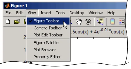
You can access or remove the figure toolbars and the plotting tools from the
Viewmenu, as shown in the following picture. Toggle on and off the toolbars you need. Adding a toolbar stacks it beneath the lowest one.
[image:67.558.145.410.158.298.2]Figure Toolbars
Figure toolbars provide easy access to many graph modification features. There are three toolbars. When you place the cursor over a particular tool, a text box pops up with the tool name. The following picture shows the three toolbars displayed with the cursor over theData Cursortool.
Plotting Tools
Plotting tools are attached to figures and create an environment for creating graphs. These tools enable you to perform the following tasks:
• Select from a wide variety of graph types.
• Change the type of graph that represents a variable.
• See and set the properties of graphics objects.
• Annotate graphs with text, arrows, etc.
• Create and arrange subplots in the figure.
• Drag and drop data into graphs.
Display the plotting tools from theViewmenu or by clicking theShow Plot Toolsicon in the figure toolbar, as shown in the following picture.
Enable plotting tools from the View menu or toolbar
You can also start the plotting tools from the MATLAB prompt:
plottools
The plotting tools are made up of three independent GUI components:
Overview of Plotting
• Plot Browser — Select objects in the graphics hierarchy, control visibility, and add data to axes.
• Property Editor — Change key properties of the selected object. ClickMore Propertiesto access all object properties with the Property Inspector.
You can also control these components from the Command Window, by typing the following:
figurepalette plotbrowser propertyeditor
See the reference pages forplottools,figurepalette,plotbrowser, and
propertyeditorfor information on syntax and options.
Using Plotting Tools and MATLAB Code
You can enable the plotting tools for any graph, even one created using MATLAB commands. For example, suppose you type the following code to create a graph:
t = 0:pi/20:2*pi; y = exp(sin(t));
plotyy(t,y,t,y,'plot','stem') xlabel('X Axis')
Overview of Plotting
title('Two Y Axes')
This graph contains twoy-axes, one for each plot type (a lineseries and a stemseries). The plotting tools make it easy to select any of the objects that the graph contains and modify their properties.
Arranging Graphs Within a Figure
Overview of Plotting
Click to add one axes to bottom of current layout.
Click and drag right to specify axes layout.
Select the axes you want to target for plotting. You can also use thesubplot
function to create multiple axes.
Choosing a Type of Graph to Plot
Creating Graphs with the Plot Selector
After you select variables in the Workspace Browser, you can create a graph
of the data by clicking the Plot Selector toolbar button. The Plot Selector icon depicts the type of graph it creates by default. The default graph reflects the variables you select and your history of using the tool. The Plot Selector icon changes to indicate the default type of graph along with the function’s name and calling arguments. If you click the icon, the Plot Selector executes that code to create a graph of the type it displays. For example, when you select two vectors namedtandy, the Plot Selector initially displays
plot(t,y).
Overview of Plotting
You can see how the graph is created because the code the Plot Selector generates executes in the Command Window:
>> area(t,y,'DisplayName','t,y');figure(gcf)
Overview of Plotting
To keep the help text visible, click just inside the top edge of the pop-up help window and drag it to another location on your screen. Close the window by clicking on theXin its upper left corner.
For more information about using the Plot Selector, see “Creating Plots from the Workspace Browser”.
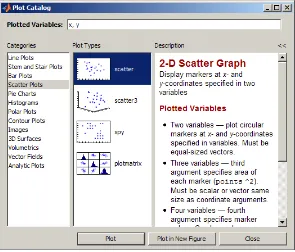
Creating Graphs with the Plot Catalog
Open the Plot Catalog in any of the following ways:
• Open the Plot Selector menu and click theCataloglink at the bottom of the menu.
• In the Workspace browser, right-click a selected variable and choosePlot Catalogfrom the context menu.
• In the Variable Editor, select the values you want to graph, right- click the selection you just made, and choosePlot Catalogfrom the context menu.
• If you are using the Figure Palette (a component of the Plotting Tools), right-click a selected variable and choosePlot Catalogfrom the context menu
[image:78.558.145.440.91.343.2]Overview of Plotting
The menu of plot types above thePlot Catalogitem is the same as your current Plot Selector list of “favorites.” This means that you can specify these items to be the kinds of graphs that you regularly use. See “Working with the Plot Selector GUI” for more information on managing a list of favorite graph types.
Select a category of graphs and then choose a specific type.
Specify variables to plot. See a description of each plot type.
Editing Plots
Editing Plots
In this section...
“Plot Edit Mode” on page 3-23
“Using Functions to Edit Graphs” on page 3-28
Plot Edit Mode
Plot edit mode lets you select specific objects in a graph and enables you to perform point-and-click editing of most of them.
Enabling Plot Edit Mode
To enable plot edit mode, click the arrowhead in the figure toolbar:
Plot edit mode enabled
You can also selectEdit Plotfrom the figureToolsmenu.
Setting Object Properties
After you have enabled plot edit mode, you can select objects by clicking them in the graph. Selection handles appear and indicate that the object is selected. Select multiple objects usingShift+click.
The context menu provides quick access to the most commonly used operations and properties.
Using the Property Editor
Editing Plots
Click to display Property Inspector
Accessing Properties with the Property Inspector
TheProperty Inspectoris a tool that enables you to access most Handle Graphics properties and other MATLAB objects. If you do not find the property you want to set in the Property Editor, click theMore Properties
button to display the Property Inspector. You can also use theinspect
command to start the Property Inspector. For example, to inspect the properties of the current axes, type
The following picture shows the Property Inspector displaying the properties of a graph’s axes. It lists each property and provides a text field or other appropriate device (such as a color picker) from which you can set the value of the property.
Editing Plots
The Property Inspector lists properties alphabetically by default. However, you can group Handle Graphics objects, such as axes, by categories which you
can reveal or close in the Property Inspector. To do so, click the icon at the upper left, then click the + next to the category you want to expand. For example, to see the position-related properties, click the+to the left of thePositioncategory.
Using Functions to Edit Graphs
Some Ways to Use Plotting Tools
Some Ways to Use Plotting Tools
In this section...
“Plotting Two Variables with Plotting Tools” on page 3-29
“Changing the Appearance of Lines and Markers” on page 3-32
“Adding More Data to the Graph” on page 3-33
“Changing the Type of Graph” on page 3-36
“Modifying the Graph Data Source” on page 3-38
Plotting Two Variables with Plotting Tools
Suppose you want to graph the functiony = x3over thexdomain -1 to 1. The
first step is to generate the data to plot.
It is simple to evaluate a function like this because the MATLAB software can distribute arithmetic operations over all elements of a multivalued variable.
For example, the following statement creates a variablexthat contains values ranging from -1 to 1 in increments of 0.1 (you could also use thelinspace
function to generate data forx). The second statement raises each value in
xto the third power and stores these values iny:
x = -1:.1:1; % Define the range of x
y = x.^3; % Raise each element in x to the third power
Now that you have generated some data, you can plot it using the MATLAB plotting tools. To start the plotting tools, type
plottools
Some Ways to Use Plotting Tools
Note When you invokeplottools, the set of plotting tools you see and their relative positions depend on how they were configured the last time you used them. Also, sometimes when you dock and undock figures with plotting tools attached, the size or proportions of the various components can change, and you may need to resize one or more of the tool panes.
Selectplot(x, y)from the menu. The line graph plots in the figure area. The black squares indicate that the line is selected and you can edit its properties with the Property Editor.
Changing the Appearance of Lines and Markers
Next, change the line properties so that the graph displays only the data point. Use the Property Editor to set following properties:
• Line to no line
• Marker to o (circle)
• Marker size to 4.0