T H E J O U R N A L O F H U M A N R E S O U R C E S • 47 • 3
Estimating Teacher Value-Added and its
Persistence
Josh Kinsler
A B S T R A C T
The levels and growth achievement functions make extreme and diametri-cally opposed assumptions about the rate at which teacher inputs persist. I first show that if these assumptions are incorrect, teacher value-added esti-mates can be significantly biased. I then develop a tractable, cumulative model of student achievement that allows for the joint estimation of unob-served teacher quality and its persistence. The model can accommodate varying persistence rates, student heterogeneity, and time-varying teacher attributes. I implement the proposed methodology using schooling data from North Carolina, and find that only a third of the contemporaneous teacher effect survives into the next grade.
I. Introduction
Teacher quality is widely believed to be the most important school-level input into the production of student achievement. However, quantifying the amount of variation in student test scores that can be attributed to differing teacher assignments is difficult since teacher ability is largely unobservable.1To overcome
this hurdle, researchers often treat teacher quality as an unobserved parameter to be estimated directly using student test-score variation across classrooms and over time.2 This approach, widely known as value-added modeling, has two primary benefits. First, value-added models provide an objective, teacher-specific measure of
1. Observable teacher characteristics, such as education, experience, and licensure, have been shown to have limited predictive power for student outcomes. See Hanushek and Rivkin (2006) for a review of this literature.
2. Sanders, Saxton, and Horn (1997) were the first to develop and employ a value-added framework.
Josh Kinsler is an assistant professor of economics at the University of Rochester. The author would like to thank seminar participants at NYU, the University of Western Ontario, and participants at the 34th Annual AEFP Conference. The author also wishes to thank Peter Arcidiacono, Ronni Pavan, and Nese Yildiz for helpful comments. Researchers may acquire the data used in this article from the North Caro-lina Education Research Data Center http://childandfamilypolicy.duke.edu/project_detail.php?id=35. For questions regarding the data, contact Josh Kinsler, joshua.kinsler@rochester.edu.
[Submitted November 2010; accepted July 2011]
effectiveness that many favor over subjective measures such as principal or peer evaluations. Second, value-added models allow researchers to trace out the entire distribution of teacher quality, which is useful for determining how much of the gaps in student outcomes can be attributed to variable school inputs. Although the benefits of the value-added approach are clear, considerable debate remains about whether these models can consistently estimate teacher effectiveness.
The controversy surrounding the use of value-added models is in part related to the fact that there is no benchmark methodology. Value-added modeling is a broad term that encompasses a variety of approaches that share one common feature, mea-suring the effectiveness of individual teachers using student test scores.3However,
the various approaches within the broader value-added framework often make con-flicting assumptions regarding the underlying achievement production function. In particular, assumptions about how teacher inputs persist over time are often dia-metrically opposed. As an example, three of the most widely cited papers that es-timate the distribution of teacher quality make drastically different assumptions re-garding the persistence of teacher inputs. Rockoff (2004) assumes that teacher inputs do not persist at all, identifying teacher effectiveness using variation in the level of student test scores. Hanushek, Kain, and Rivkin (2005) make the exact opposite assumption, perfect persistence from one year to the next, when they use variation in test-score growth to estimate contemporaneous teacher effectiveness. Finally, Aa-ronson, Barrow, and Sander (2007) take a middle ground and assume that teacher inputs, along with all other inputs including student ability, persist at a constant geometric rate.
Despite the significant differences in approach, the basic findings across all three aforementioned studies are quite similar. A one standard deviation increase in teacher quality yields approximately 10 percent of a standard deviation increase in math test scores and slightly smaller effects in reading. The obvious question given the sim-ilarity in results across the various specifications is whether the assumptions about teacher persistence actually matter. Using theoretical and empirical examples I show that incorrect persistence assumptions can lead to significant biases in estimates of individual teacher value-added and dispersion in teacher value-added. The magnitude of the biases depend on how students and teachers are sorted across schools and classrooms and how poor the initial persistence assumptions are. In particular, the bias in estimates of teacher added tend be large when the true teacher value-added experienced by each student is highly correlated across grades, either posi-tively or negaposi-tively. Additionally, the growth model will tend to perform well when the true persistence rate is close to one, while the levels model will tend to perform well when the true persistence rate is close to zero.
Uncertainty about the actual rate at which teacher inputs persist has led to a number of recent papers that estimate the depreciation rate directly. In a lag score model, Jacob, Lefgren, and Sims (2010) and Kane and Staiger (2008) show that using either an indicator or the actual measure of the lagged teacher quality as an instrument for the lagged test score yields an estimate of teacher persistence. Across the two papers, estimates of teacher persistence range between 0.15 and 0.5.
ever, neither paper estimates the decay rate jointly with teacher quality, which can lead to potential biases in both parameters. Lockwood et al. (2007) jointly estimate teacher quality and the rate of persistence using Bayesian MCMC techniques. Es-timated decay rates are quite small; however, the model does not account for any observed or unobserved variation in student quality. Finally, Rothstein (2010) esti-mates a cumulative model that allows teachers to have separate contemporaneous and future effects.4The rate of persistence, estimated between 0.3 and 0.5, can be recovered in a second step by comparing the average relationship between the con-temporaneous and future effect for each teacher. However, computational challenges severely limit both the estimation sample and production technology employed.
In this paper, I add to the above literature by developing and estimating a simple, but comprehensive, cumulative production technology that jointly estimates teacher quality and persistence. The proposed achievement model is flexible along many dimensions. Individual teacher quality is treated as a time-invariant unobserved pa-rameter to be estimated; however, teacher effectiveness can vary over time as teach-ers accumulate experience and additional schooling. The rate at which teacher inputs persist can be geometric, or can vary across grades or over time in a more flexible fashion. The model can be estimated in either achievement levels or growth and can accommodate unobserved student heterogeneity in ability in either context. Contem-poraneous and lagged observable student and classroom attributes also can be in-corporated.
Despite the potentially large number of teacher and student parameters, the model can be computed in a timely manner. Rather than estimate all the parameters in one step, I take an iterative approach that toggles between estimating teacher persistence, teacher heterogeneity, student heterogeneity, and any remaining parameters.5Each
iteration is extremely fast since I use the first-order conditions generated from min-imizing the sum of the squared prediction errors to estimate the teacher and student heterogeneity directly. The iterative procedure continues until the parameters con-verge, at which point the minimum of the least squares problem has been achieved. With a sample of over 600,000 students and 30,000 teachers I can estimate the baseline model in less than 15 minutes.
Using student data from North Carolina’s elementary schools I implement the proposed cumulative model and find that teacher value-added decays quickly, at rates approximately equal to 0.35 for both math and reading. A one standard deviation increase in teacher quality is equivalent to 24 percent of a standard deviation in math test scores and 14 percent of a standard deviation in reading test score. These results are consistent with previous evidence regarding the magnitude of teacher value-added and the persistence of teacher inputs. Using the levels or growth frame-works instead results in biases in the variance of teacher value-added on the order of 4 percent and 7 percent respectively for math test-score outcomes, and smaller biases in reading outcomes. However, the somewhat small biases in the variance of overall teacher value-added masks larger within-grade biases that are on the order
4. Carrell and West (2010) take a similar approach when measuring the short- and long-term effectiveness of professors at the college level. In contrast to the findings from Rothstein (2010) and Jacob, Lefgren, and Sims (2010) at the elementary school levels, they find that the short- and long-term effects are actually negatively correlated.
of 15 percent. The individual estimates of teacher quality from the cumulative model and the levels model are very highly correlated, while the growth model estimates individual teacher value-added less accurately. In general, the similarities in teacher value-added across the cumulative, levels, and growth models in the North Carolina sample reflect the fact that for the average student, teacher value-added is only marginally correlated across grades.
The remainder of the paper is as follows. The pitfalls of the levels and growth frameworks are illustrated in Section II. Section III outlines a cumulative production function that allows for flexible persistence patterns, discusses identification of the key parameters, and provides an estimation methodology. Section IV introduces the North Carolina student data used to estimate the cumulative production function. Section V contains analysis of the model results and Section VI concludes.
II. Persistence Assumptions and Estimates of Teacher
Quality
The most common value-added models of teacher quality assume that teacher effects either persist forever or not at all. The motivation for making these extreme assumptions is typically model tractability. Consider the following two achievement equations:
A =α +
∑
I T +ε(1) ijg i ijg jg ijg ∈
j Jg
A −A =
∑
I T +e(2) ijg ij′g′ ijg jg ijg ∈
j Jg
whereAijgis the achievement outcome for student matched with teacher in gradei j
. is the set of all grade teachers and is an indicator function that takes on
g Jg g Iijg
the value of one if studentiis matched with teacherjin grade .g Tjg is the value-added of teacher j in gradeg andαiis the grade-invariant ability level of student
.
i
Both Equations 1 and 2 allow for unobserved student ability to affect the level of individual test scores. Equation 1 is a simplified version of the levels specification employed in Rockoff (2004), which implicitly assumes that grade g’s outcome is entirely unaffected by teachers in previous grades. Equation 2 is a growth equation that can be generated by first differencing two levels scores. However, in order for only the contemporaneous teacher to enter in the equation, past teacher inputs must persist perfectly. The key benefit to either of the extreme assumptions about teacher persistence is that only one set of teacher effects enters into Equations (1) and (2), making estimation relatively straightforward. However, as I show below, these ex-treme assumptions can have significant consequences for both ˆ and ˆ2.
Tjg σT
growth or levels framework. However, because the lag-score model is typically im-plemented without controls for unobserved student heterogeneity, the coefficient on the lag score is typically quite high, on the order of 0.8. This implies that past teacher inputs also decay at a rate equal to 0.8. Thus, I suspect that the pattern of biases in the lag-score framework are best approximated by the biases in the growth model.
A. Theoretical Example
Assume that we observe three test-score outcomes for each of three different stu-dents, denotedAig whereiindexes students andg indexes grade or time. The three students are all members of the same school. The first test-score observation for each student is not associated with any teacher and can be considered an unbiased measure of a student’s unobserved ability. This assumption is useful since it ensures that all the student and teacher parameters will be separately identified and is also consistent with the data to be used in the empirical analysis. In the remaining two grades, students are assigned to one of two teachers that are unique to each grade, whereTjg is the th teacher in grade . Thus, there are four teachers in the school:j g
, , , and . As an example, the set of outcomes for student 1 takes the
T12 T22 T13 T23
following form:
A =α
(3) 11 1
A =α +T
(4) 12 1 12
A =α +T +δT
(5) 13 1 13 12
In order for δto be identified, students must switch classmates in Grade 3, gen-erating variation inTj2for one of the Grade 3 teachers. I assume that students 2 and 3 are assigned teacher T22 in Grade 2 and students 1 and 2 are assigned teacher in Grade 3. The singleton student classes are matched with teachers and
T13 T12
. All of the unobserved parameters, , , and are identified in this simple
T23 αi δ Tjg
system. Since I have written the achievement outcomes without any measurement error, it is possible to pin down exactly each of the unobserved parameters. The question is what happens to the estimates of Tˆ andσˆ2 when we assume that δ
jg jg
equals either 0 or 1.
To derive the least squares solutions for ˆTjg when δ is assumed to equal 0, I simply differentiate the squared deviations and solve for the parameters as a function of Aig, the only observables in the model. I then substitute back in the true data generating process for Aig to illustrate how the estimates differ from the true un-derlying parameters. In the levels case,δ= 0, the least squares estimates of the four teacher effects is given by
4δ L
ˆT12=T12− (T12−T22)
15 2δ L
ˆT22=T22+ (T12−T22)
15 δ L
δ L
ˆT23=T23+ (T12+ 14T22) 15
The first thing to notice is that unlessδ equals zero all of the estimates of teacher quality will be biased, even the Grade 2 teacher effects. The bias in the Grade 2 teacher effects arises because the unobserved student abilities adjust to account for the unexplained variance in the third grade outcome. This in turn leads to bias in all the teacher effect estimates. The teacher effects in second grade are always biased toward the average effect, while the bias in the third grade teacher effects depend on whether or not T12and T22 are greater than zero. If the second grade teachers are “good,” then the estimated effects of the Grade 3 teachers will be biased upward since they receive some credit for the lingering effects of the previous grade’s teacher. The opposite result is true if the second grade teachers are “bad.” Thus, teachers following excellent teachers will be unjustly rewarded while teachers fol-lowing a string of poor teachers are unjustly penalized in a model that incorrectly assumes no persistence.
Not only are the individual estimates of teacher quality biased, but the overall distribution of teacher quality is also affected. Because the Grade 2 teacher effects are always biased toward the average effect, σˆ2 will be biased toward zero. The
j2
bias in the estimated dispersion of the Grade 3 teacher effects is given by
2
4δ
2 2 2
ˆ
σ −σ = (T −T ) + 20δ(T −T )(T −T )
(6) j3 j3 12 22 13 23 12 22
50
The first term on the right hand side of the above expression is positive for any rate of persistence. However, the second term can be either positive or negative depend-ing on the correlation in teacher quality across time periods. In this simple example the cross-grade correlations in teacher quality are weighted equally. However, with more students and teachers, the weight given to each cross-grade correlation will depend on how many students are associated with each teacher pair. Thus, depending on how students are tracked through classes, the bias inσˆ2 could be either positive
j3
or negative. If the bias in the the variance of the third grade teacher effects is large enough, it could swamp the bias in the estimate of teacher dispersion in second grade, leading to an inconclusive overall bias in the variance of teacher quality.
Rather than assume δ= 0, we could instead assume that δ= 1 and estimate a simple growth score model with two observations per student. In this case the biases work quite differently. Because the student fixed effects are differenced out of the model, there is nothing to cause bias in the Grade 2 teacher effects. As a result, .6However, the estimated Grade 3 teacher effects will be biased as a result
G
ˆTj2=Tj2
of the incorrect assumptions about the persistence of the Grade 2 teachers. In par-ticular,
1 G
ˆT13=T13+ (δ−1)(T12+T22)
2
G
ˆT23=T23+ (δ−1)T22
Clearly if δ= 1 neither teacher effect is biased. Otherwise, both Grade 3 teacher effects will be biased in a direction that again depends on the quality of the Grade 2 teacher. In contrast to the levels model, following an excellent Grade 2 teacher will bias downward the Grade 3 teacher effect since excess credit is given to the previous teacher. Thus, the teachers that get unjustly rewarded in the levels model are the same teachers who get unjustly punished in the growth framework.
The bias in the estimates of the Grade 3 teacher effects bleeds into the estimate of the overall dispersion of teacher quality. The bias in the estimated variance of Grade 3 teacher quality is given by
1
2 2 2 2
ˆ
σ −σ = ((δ−1) (T −T ) + 4(δ−1)(T −T )(T −T ))
(7) j3 j3 12 22 13 23 12 22
8
The first term inside the parentheses is always positive while the sign of the second term will depend on the cross-grade covariances in teacher quality. Again, in a model with more students and teachers, the weight given to the cross-grade teacher covar-iance terms will depend on the number of students associated with each teacher pair. If teacher ability is correlated across grades at the student level, the dispersion in teacher quality in the growth framework will be understated since(δ−1)is negative. This is the opposite of the bias in the levels framework.
The simple example above highlights a number of important issues regarding the standard levels and growth models employed to evaluate teachers. First, when teacher effects persist, the levels model yields biased estimates of all teacher effects, including the initial teacher. Second, the bias in the estimated dispersion in teacher quality varies significantly across grades, particularly in the levels framework. Fi-nally, the bias in the individual estimates of teacher quality and overall dispersion in teacher quality depend critically on how students and teachers are tracked across grades. The next section illustrates this final point by examining empirically the magnitude of the biases under various sorting scenarios.
B. Empirical Exercise
The purpose of this section is to illustrate the magnitude of the biases in the dis-persion of teacher quality under various teacher and student sorting scenarios. I expand the simple model from the previous section and generate a data set that is representative of the type of schooling data available to researchers. I assume that there are 25 schools in the sample and 5,000 students. For each student, a baseline test-score measure is available, followed by three classroom test-score observations associated with a particular grade, say Grades 3, 4, and 5. Within each school, there are four teachers per grade, and each teacher is observed with 50 students. I continue to assume that the achievement tests are perfect measures of student knowledge, primarily to illustrate that any biases that emerge are strictly a result of model misspecification.
assume that student ability is distributedN(0,1)and that teacher quality is distributed .7The distribution of teacher quality is identical across the three grades.
N(0,0.0625)
The final and most important decision when generating the data is how to dis-tribute students and teachers to schools and classrooms. As the previous section highlights, the bias in the dispersion of teacher quality will depend to a large extent on the cross-grade correlations in teacher quality at the student level. There are two methods for generating cross-grade correlations in teacher quality: sorting of students to teachers within schools, and sorting of teachers across schools. Within schools, if individual students are consistently matched with either relatively high- or low-ability teachers, then teacher quality will be positively correlated across grades. A negative correlation would result if principals, in an attempt at fairness, assign a relatively high-ability teacher one year followed by a relatively low-ability teacher the next. Even if there exists no sorting within schools, teacher ability will correlated across grades if teachers sort across schools based on ability. Regardless of the source of the cross-grade correlation in teacher quality, the previous section suggests that the estimated dispersion in teacher quality will be significantly impacted.8
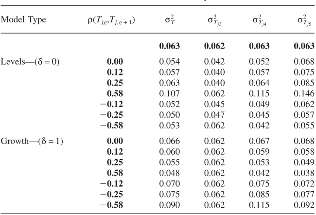
Table 1 illustrates how the estimated dispersion in teacher quality from both the levels and growth models are affected by varying amounts of cross-grade correlation in teacher ability.9Within each model type, levels, or growth, the first row contains
the estimates of teacher dispersion when there is no cross-grade correlation in teacher quality, followed by three levels of positive and negative sorting.10The results are
averages over 500 simulations where the underlying population of students and teachers is held fixed, and only the sorting of students to teachers within schools changes with each iteration.
The pattern of results is quite consistent with the predictions from the simple theoretical exercise. The bias in the estimated variance of teacher quality varies significantly across grades for all types of sorting, particularly in the levels frame-work. In the growth model, the variance of third grade teacher quality is always perfectly identified, regardless of how students and teachers are sorted. The direc-tions of the bias in the levels and growth models is as expected. With no cross grade correlation in teacher quality, the overall variance in teacher value-added is biased downward in the levels framework and upward in the growth framework. These biases are generated by the fact that past teachers are an omitted variable in the contemporaneous outcomes. With negative sorting these patterns are exaggerated, and with significant positive sorting these biases are flipped. With extreme levels of positive (negative) sorting, the estimated variance of teacher value-added is biased upward in the levels (growth) model by 72 percent (43 percent).
7. The dispersion in student ability and teacher quality is similar to those estimated using data from North Carolina.
8. If an unbiased measure of student ability were unavailable, only within-school variation in teacher quality would be identified. In this case the source of the cross-grade correlation in teacher quality would matter since if it was generated all by teacher sorting across schools, the within-school estimates of dis-persion would be unaffected.
9. I chose the cross-grade correlations in an effort to illustrate the performance of the levels and growth models across a spectrum of potential realizations. For the North Carolina data, it turns out that the cross-grade correlation in teacher quality is approximately 0.11.
Table 1
Estimating Variance in Teacher Ability using Misspecified Levels and Growth Models
True Persistence of Teacher Ability:δ= 0.5 Model Type ρ(Tjg,Tj,g+ 1)
2
σT
2
σTj3
2
σTj4
2
σTj5
0.063 0.062 0.063 0.063
Levels—(δ= 0) 0.00 0.054 0.042 0.052 0.068
0.12 0.057 0.040 0.057 0.075
0.25 0.063 0.040 0.064 0.085
0.58 0.107 0.062 0.115 0.146
−0.12 0.052 0.045 0.049 0.062
−0.25 0.050 0.047 0.045 0.057
−0.58 0.053 0.062 0.042 0.055
Growth—(δ= 1) 0.00 0.066 0.062 0.067 0.068
0.12 0.060 0.062 0.059 0.058
0.25 0.055 0.062 0.053 0.049
0.58 0.048 0.062 0.042 0.038
−0.12 0.070 0.062 0.075 0.072
−0.25 0.075 0.062 0.085 0.077
−0.58 0.090 0.062 0.115 0.092
Note: Results are averages over 500 simulations. Generated sample contains 25 schools, 3 grades per school, and 4 teachers per grade. Each teacher is observed with 50 students. Student and teacher ability are unobserved. Grades are generated according to a cumulative achievement equation where teacher inputs persist at a constant geometric rate equal to 0.5. Students are observed four times, first without any associated teacher, and then once in each grade. There is no additional measurement error in the model so that any biases stem entirely from model misspecification. Teacher and student populations are held fixed across the simulations, with only the within school sorting of students to teachers changing.Tjgis the ability of teacherjin gradeg.ρ(T ,T ) is the correlation in teacher quality across grades.σ2is the
jg j,g+ 1 T
true variance of teacher ability across all grades, while 2 is the true variance of ability for third grade σTj3
teachers only. The levels model implicitly assumes a persistence rate of 0 while the growth model implicitly assumes a persistence rate of 1. Bold-faced numbers reflect true underlying distributions.
Not only are the estimates of the dispersion in teacher quality affected by the strong persistence assumptions inherent in the growth and levels framework, the individual estimates of teacher quality are also affected. For each of the simulations, I also calculated the proportion of schools that were able to successfully identify the best teacher within each grade. Under random assignment, both models actually perform well, identifying the best teacher in all grades more than 95 percent of the time. When the cross-grade correlation in teacher quality is equal to 0.25, the levels model continues to perform quite well, however the growth model identifies the best fourth and fifth grade only 83 percent and 74 percent of the time respectively. When the cross-grade correlation in teacher quality is equal to −0.25 performance is
grade, while the levels model only identifies the best teacher in fourth and fifth grade 87 percent of the time.
The intuition for the difference in the ability of the levels and growth models to identify the best teacher in each grade is the following. With positive sorting, the best (worst) fourth grade teacher tends to follow the best (worst) third grade teacher. Because the levels model assumes that the third grade teacher has no effect in fourth grade, the impact of the best (worst) fourth grade teacher will be biased upward (downward). This tends to increase the estimated dispersion in teacher quality, while maintaining the relative rank of each teacher. As a result, the correlation between the estimated teacher value-added and the truth is high. In the growth framework, if teacher quality is positively correlated across grades, the effect of the best (worst) fourth grade teacher is biased downward (upward). The best fourth grade teacher follows the best third grade teacher, who continues to get significant credit for fourth grade performance since it is assumed that teacher effects persist forever. The esti-mated dispersion in teacher quality will be reduced and the ranking of teachers becomes significantly more jumbled. The stronger the positive correlation and the closerδ is to zero the more jumbled the ranking would become. If the true corre-lation in teacher value-added across grades were negative, the opposite would hold. The estimated teacher value-added from the growth (levels) framework would be highly (lowly) correlated with the truth.
Overall the results from this simple empirical exercise illustrate that both the levels and growth models are likely to be biased, though the direction and the severity will depend on how teachers and students are sorted across schools and classrooms.11
The concern is that the extent of sorting on unobserved teacher and student ability is unknown a priori, thus leaving researchers with little guidance about which model will work best in particular situations. Rather than make strong and potentially in-correct assumptions about the persistence of teacher quality, I develop a straightfor-ward method of estimating both teacher value-added and the rate at which teacher inputs persist.
III. Estimating Persistence
In the following sections, I lay out a methodology for estimating a cumulative production function for student achievement that yields estimates of teacher quality and the rate at which teacher inputs persist. I start with a baseline model that contains only unobserved student ability, teacher effects, and the
tence parameter.12Within this simple framework I discuss identification, estimation,
consistency, and important assumptions regarding the assignment of students to teachers. I then extend the basic model to allow for heterogenous decay rates and time-varying teacher quality. Finally, I provide some Monte Carlo evidence that illustrates the accuracy of the proposed estimation methodology.
A. Baseline Model
The biases in the teacher-specific measures of effectiveness and the overall disper-sion in teacher quality stemming from incorrect assumptions about input persistence can be avoided by instead jointly estimating teacher quality and the persistence of teacher inputs. Expanding on the simple cumulative specification outlined in Equa-tions 3–5, assume that the true achievement production function is given by
g−1
g−g′
A =α +
∑
I T +∑
δ (∑
I T ) +ε(8) ijg i ijg jg ijg′ jg′ ijg
∈ ∈
j Jg g′= 1 j Jg′
whereIijgis an indicator function that equals one when student is assigned teacheri
in grade , and is the set of all grade teachers. represents measurement
j g Jg g εijg
error in the test’s ability to reveal a student’s true underlying knowledge, and is uncorrelated with unobserved student ability and teacher assignments in all periods. I return to the issue of exogeneity at the conclusion of this section.
The first summation in achievement equation is the effect of the contemporaneous teacher, while the second summation accounts for the discounted cumulative impact of all the teachers in grades g′<g. For simplicity, I assume here that the teacher inputs persist at a constant geometric rate δ, though I will relax this assumption later. The lingering impact of past teachers is assumed to be proportional to their contemporaneous impact. In practice, I could allow teachers to have separate con-temporaneous and long-term effects rather than estimate a mean persistence rate, similar to Rothstein (2010). However, I choose to measure teacher effectiveness with one parameter that captures a mixture of both effects.
Prior to discussing estimation, it is useful to briefly describe the variation in the data that identifiesδ. As long as students are not perfectly tracked from one grade to the next, conditional on the current teacher assignment there will be variation in the lagged teacher. In practice, perfect tracking is rarely employed, and thus iden-tification is obtained.
Estimation, on the other hand, is complicated by both the multiple sets of high-dimensional teacher fixed effects and the inherent nonlinearity stemming from the interaction between the persistence parameter and the teacher effects. To deal with these issues, I pursue an iterative estimation strategy similar in spirit to the one out-lined in Arcidiacono et al. (Forthcoming). Define the least squares estimation problem as,
N g¯ g−1
g−g′ 2
min
∑ ∑
(A −α−∑
I T −∑
δ (∑
I T ))(9) ijg i ijg jg ijg′ jg′
α,T,δi= 1g=g j∈Jg g′= 1 j∈Jg′ ¯
where , , and are the parameters of interest, andg
¯
and are the minimum and
α T δ g¯
maximum grades for which test score are available. The iterative estimation method toggles between estimating (or updating) each parameter vector taking the other sets of parameters as given. At each step in the process the sum of squared errors is decreased, eventually leading to the least squares solution.13
In practice, estimation proceeds according to the steps listed below. The algorithm begins with an initial guess for α andT and then iterates on three steps, with the
th iteration given by:14 q
• Step 1: Conditional onαq−1andTq−1, estimateδqby nonlinear least squares. • Step 2: Conditional on δq andTq−1, update αq.
• Step 3: Conditional on αq andδq, updateTq.
The first step is rather self-explanatory, however the second and third steps require some explanation since it is not clear what updating means. To avoid having to “estimate” all of the fixed effects, I use the solutions to the first-order conditions with respect toα andTto update these parameters.
The derivative of the least squares problem with respectαifor alli is given by the following
g¯ g−1
g−g′
∑
(A −α−∑
I T −∑
δ (∑
I T ))(10) ijg i ijg jg ijg′ jg′
∈ ∈
g=g j Jg g′= 1 j Jg′ ¯
Setting this equal to zero and solving for αiyields
g¯ g−1
g−g′
∑
(Aijg−∑
IijgTjg−∑
δ (∑
Iijg′Tjg′))∈ ∈
g=g j Jg g′= 1 j Jg′
¯
α = (11) i
g¯−g ¯
which is essentially the average of the test-score residuals purged of individual ability. To update the full vector of abilities in Step 2, simply plug the th estimateq
ofδand theq−1step estimate of T into theN ability updating equations. The strategy for updating the estimates of teacher quality in Step 3 is essentially identical to the one outlined for updatingα. The key difference is that the first-order condition for Tjg is significantly more complicated. Teachers in gradesg<g¯ will
13. Matlab code for the baseline accumulation model and a simple data generating program can be down-loaded at http://www.econ.rochester.edu/Faculty/Kinsler.html
14. My initial guess forαis the average student test score across all periods, and my initial guess forT
is the average test score residual for each teacher after controlling for student ability. When guessing , IT
have not only a contemporaneous effect on achievement outcomes, but also an effect on student outcomes going forward. Thus, test-score variation in future grades aids in identifying the quality of each teacher. The first-order condition of the least squares problem in Equation 9 with respect to , for
¯
, is
Tjg g<g<g¯
g−1
∑
[(
A −α−T −∑
I T )(12) ijg i jg ijg′ jg′
∈
i Nijg g′= 1
g
¯ g′−1
g′−g g′−g″
+
∑
δ (Aijg′−αi−∑
Iijg′Tjg′−∑
δ Iijg″Tjg″)] ∈g′=g+ 1 j Jg′ g″= 1
where Nijg are the set of all students who are assigned teacherj in grade g. The first term inside the summation overi comes from the contemporaneous effect of . The second term inside the summation accounts for the effect of in all
Tjg Tjg
subsequent grades. Notice thatTjg appears in the final summation of Equation 12 since at some pointg″will equal .g
Setting the first-order condition with respect toTjg equal to zero and solving for yields
Tjg
g−1
∑
[
Aijg−αi−∑
Iijg′Tjg′]
∈i Nijg g′= 1
T =
(13) jg g¯
2(g′−g)
∑
(1 +∑
δ ) ∈i Nijg g′=g+ 1
g¯ g′−1
g′−g g′−g″
∑
[
∑
δ (Aijg′−αi−∑
Iijg′Tjg′−∑
δ Iijg″Tjg″)]∈ ∈
i Nijg g′=g+ 1 j Jg′ g″= 1,g″⬆g
+ g¯
2(g′−g)
∑
(1 +∑
δ ) ∈i Nijg g′=g+ 1
where I split the term into two pieces for ease of presentation even though they share a common denominator. Again, the first term uses information from grade g
to identifyTjg, while the second term uses information from grades g′>g. Notice that the equation for T includes T for g′⬆g. Thus, updating T in Step 3
jg jg′ jg
requires substituting in theqth iteration estimates ofα andδ, as well as theq−1 step estimates ofT into Equation 13.15
jg′
Iterating on Steps 1–3 until the parameters converge will yield the αˆ,Tˆ, and δˆ that solve the least squares problem outlined in Equation 9. At this point it is useful to step back and consider whether these are consistent estimators of the underlying parameters of interest. Because each student is observed at most
¯times, the ˆ
g¯−g α
will be unbiased, but inconsistent. This is a standard result in panel data models with largeN fixed T, where Nrefers to the number of students and Trefers to the number of observations per student. The estimates of teacher effectiveness,Tˆ, are consistent estimators of T if the number of student test-score observations per teacher goes to infinity as Nr⬁. This would be achieved, for example, if each
entering cohort of students experienced the same teacher population. In this case, consistency ofTˆ would then imply consistency ofδˆ. In practice, however, teachers move in and out of the profession, making it likely that as the number of students increases, so do the number of teachers. As a result, the teacher effects themselves will be inconsistent, as willδˆ. However, the Monte Carlo exercises in Section IIIC illustrate that the bias in the estimate of teacher persistence is negligible when the median number of student observations per teacher is only twenty.
The fact thatTˆ provides a noisy measure of true teacher value added has important implications for the estimate of dispersion in teacher quality. Simply using the var-iance of Tˆ as an estimate of σTˆ2 will lead to an overstatement of the variance in teacher quality sinceTˆ contains sampling error, as shown below
ˆT =T +ν (14) jg jg jg
whereνjgis the sampling error for the th teacher in grade . Assuming thatj g νjgis uncorrelated with T , the Var(T)ˆ is equal to σ2+σ2. A crude way to correct for
jg T ν
the sampling bias is to subtract the average sampling variance across all the teacher estimates from the overall variance of the estimated teacher effects.16 To do this
requires estimating the standard errors for all of the individual teacher effects. I accomplish this by bootstrapping the student sample with replacement and reesti-mating the model. The standard deviation of a teacher effect across the bootstrap samples provides an estimate of the teacher effectiveness standard error. The Monte Carlo exercises to follow show that this approach for recovering the dispersion in teacher quality works quite well.
The final issue I want to address in terms of the baseline model is the issue of exogeneity. At the start of this section I assumed that εijg was uncorrelated with unobserved student ability and teacher assignments in all grades, not just grade .g
One obvious concern with this assumption is if there exist time-varying student and classroom characteristics that happen to be related to the teacher assignment. In the expanded version of the model, I address this issue by allowing for observable time-varying classroom and student characteristics.17Similar to the other models in the
literature, one issue I cannot address is the extent to which parents substitute for teacher quality. In other words, if a student is assigned an ineffective teacher, the parents of that student may compensate by substituting their own time.18 To the
extent that this occurs I will understate the overall variation in teacher quality. Although sorting on observable, time-varying classroom or student attributes is simple to address, more problematic is sorting on lagged test-score outcomes. The
16. In contrast, Kane and Staiger (2008) treat each teacher effect as a random effect. The dispersion in teacher quality is estimated using the correlation in the average classroom residual across classes taught by the same teacher. The authors note that fixed effects and OLS yield very similar estimates of teacher value added in their sample.
17. Unobserved classroom-year level shocks, such as a dog barking on the day of the test, are ruled out in this framework. However, there existence would likely bias the persistence effect downward and the dispersion in teacher quality upward. The biases will depend on the variance of the classroom-year level shocks and on the extent to which teachers are observed across multiple years.
assumption thatεijgis uncorrelated with all teacher assignments in gradeg′>grules out any sorting directly onAijg. In other words, all the sorting into classrooms has to be based strictly on α.19 This is a critical assumption in all value-added papers
that employ student and teacher fixed effects in either a levels or growth framework. For the remainder of the paper I also maintain the assumption of conditional random assignment.20
B. Model Extensions
1. Heterogenous Persistence
The discussion in the previous section relied on the assumption of a constant geo-metric rate of persistence. In reality, the knowledge imparted at a certain age may matter more for future performance than inputs in other years. If this is true, it would suggest that some grades may be more critical than others and that the assignment of teachers should account for this. The baseline production function can easily accommodate this by simply indexingδby grade, as seen below.
g−1
A =α +
∑
I T +∑
δ (∑
I T ) +ε(15) ijg i ijg jg g′ ijg′ jg′ ijg
∈ ∈
j Jg g′= 1 j Jg′
The identification argument is the same, except now it is critical that students do not return to their same class configurations two or three years into the future. The steps necessary for estimation remain largely the same, except that in Step 1, I estimate multipleδ’s by nonlinear least squares. Also, in the first-order conditions forαiandTjg, theδ’s will be indexed by grade.
In addition to relaxing the homogeneity of δ, it is also possible to relax the assumption that inputs persist at a geometric rate. Teacher inputs may decay very quickly after one year, but then reach a steady state where the effects no longer decline. This would imply that teachers early in the education process have a sig-nificant long term effect on achievement growth. Schools could use this information to find the optimal teacher allocation. The production function would now take the following form
g−1
A =α +
∑
I T +∑
δ (∑
I T ) +ε(16) ijg i ijg jg g−g′ ijg′ jg′ ijg
∈ ∈
j Jg g′= 1 j Jg′
19. Rothstein (2010) develops a test for whether classroom assignments are random conditional on un-observed student ability and finds that for a cohort of North Carolina fifth graders, classroom assignments are not conditionally random. Using a different sample, Koedel and Betts (2010) show that when multiple cohorts of student test scores are utilized, conditional random assignment cannot be rejected. In addition, Kinsler (Forthcoming) shows that the proposed test in Rothstein (2010) is incorrectly sized for samples similar in size to the one he employs.
whereδis indexed according to how many periods have passed since the input was applied. Again, the estimation procedure is altered to account for the multiple dis-count rates.
The two extensions discussed in this section also help differentiate this approach for estimating teacher-value added from previous approaches that rely on lag scores, such as Aaronson, Barrow, and Sander (2007). In a lag score framework, not only is it critical that all inputs persist at the same rate, including teacher, school, and student ability, but that the persistence rate be homogenous and geometric. If this is not the case, then the standard simplification in which all past inputs drop out of the levels equation no longer holds, essentially invalidating this approach.21 2. Time-Varying Teacher Quality
With one cohort of students, it is logical to assume that a teacher’s effectiveness is fixed. However, if the model is to be estimated using multiple cohorts of students, assuming that teacher effectiveness is constant over multiple years conflicts with previous research. Teacher experience is one of the few observable characteristics that appears to influence student performance. Thus, we would expect teacher ef-fectiveness to improve across multiple cohorts, at least for the teachers with the fewest years of experience. Other examples of time-varying teacher characteristics include attainment of a graduate degree or licensure status.
The achievement production function can easily accommodate changes to teacher effectiveness that result from variation in observable teacher characteristics over time. Consider the following production function for student achievement
g−1
g−g′
A =α + ∑I (T +β X ) + ∑ (δ ( ∑ I (T +βX ))) +ε
(17) ijgt i ijgt jg 2 Tjgt ijgt′ jg′ 2 Tjg′t′ ijgt
∈ ∈
j Jg g′= 1 j Jg′
whereXTjgt are the observable characteristics of teacherTjg at time , and the indi-t
cator function is now also indexed by time. Notice that the effect of the observable teacher components enters contemporaneously and in the measure of lagged teacher effectiveness. This allows, for example, the long-run effect of a teacher to vary according to when a student is matched with that teacher. The interpretation of the unobserved teacher value-added estimates is now the expected long-term teacher effectiveness once sufficient experience, education, or licensure is obtained.
Estimation of the model with time-varying teacher characteristics continues to follow the same three steps outlined for the baseline framework. Step 1 needs to be expanded to include not just estimation of δ, but also estimation of β. The first-order conditions required for updating the student and teacher effects in Steps 2 and 3 are altered slightly to account for the time-varying teacher characteristics.
Similar to teachers, students and classrooms will vary over time in observable ways. For example, students may switch schools or repeat a grade. Both of these are likely to impact performance in a particular year. Also, class size and composition will likely vary over time for each student. Incorporating these observable attributes into the above framework follows in the same fashion as the time-varying teacher attributes. Lagged observable student or classroom characteristics can be included in the production function with their own rates of persistence.
C. Monte Carlo Evidence
As noted in Section III.A, the persistence and teacher value-added parameters are only consistent under the assumption that as the number of students grow, the popu-lation of teachers is held fixed. In reality this is unlikely to hold, as teachers tend to move in and out of the profession often. To provide some small sample evidence regarding the performance of the baseline estimator and the simple extensions out-lined in the previous sections I conduct some Monte Carlo experiments. The struc-ture of the data used for the Monte Carlo exercises is chosen to mimic as closely as possible the North Carolina primary school data that will eventually be used to estimate the model. For each model specification, baseline, heterogenous persistence, and time-varying teacher quality, I assume that the methodology for assigning stu-dents and teachers to schools and classrooms is identical. Differences only emerge when generating student outcomes since this will depend on the particular specifi-cation employed.
The basic structure of the data is as follows. I create seven cohorts of students, each containing 1,500 students. Within each cohort, students are sorted into 25 schools according to their unobserved ability, which is distributed in the population . The ratio of the average within school standard deviation in ability to the
2 N(0,.85 )
population standard deviation in ability is approximately 0.92. For each student, I assume a pretest score is available, followed by third, fourth, and fifth grade out-comes. The third through fifth grade classrooms contain 20 students each, and there are three classrooms per grade per school.
Teachers are also sorted into schools based on their unobserved quality, which is distributed in the populationN(0,.25 )2 . The ratio of the average within school stan-dard deviation in teacher quality to the population stanstan-dard deviation in teacher quality is approximately 0.87. I assume that teachers and students are sorted inde-pendently. In other words, while the best teachers tend to end up in the same school, they do not necessarily end up in the school with the best students. With each new cohort of students I assume that there is significant turnover in the teacher popula-tion. Turnover is independent of teacher ability, but not experience. This allows me to generate a skewed distribution for the number of observations per teacher, where the mean number of observations per teacher is approximately equal to 35 and the median is only 20. I maintain the sorting on teacher quality across schools even as the teachers within each school change over time.
The final component that remains is how to assign students and teachers to class-rooms within each school/grade combination. I assume that teachers and students are negatively sorted on unobserved ability and quality such that the overall corre-lation between student ability and teacher quality is approximately−0.05. I chose
this to match the results obtained with my estimation sample. Note that both the negative correlation between student and teacher ability at the classroom level and the sorting of teachers into schools tends to generate positive correlation in teacher quality across grades. Recall that this is the source of the bias in teacher value-added estimates generated by the levels and growth models.
error is independently and identically distributed across grades according to . Finally, in an effort to mimic actual data conditions, I assume that some
2
N(0,.45 )
of the student test scores are missing. If a student’s fifth grade score is missing, for example, then this student cannot help identify the effectiveness of the assigned fifth grade teacher. However, if a student’s third grade score is missing, this student still aids in identifying the third grade teacher effect since the third grade teacher con-tinues to impact that student’s test-score outcomes in Grades 4 and 5.
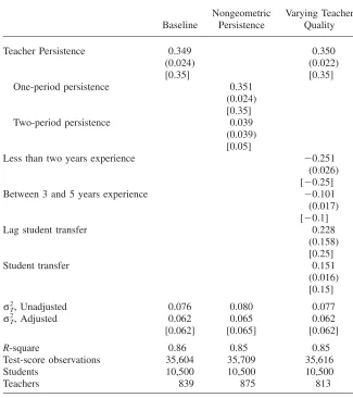
Table 2 shows the results of the Monte Carlo experiments for the baseline model, nongeometric decay, and time-varying teacher quality models. The first column of results show that in the baseline model, the teacher persistence parameter and the dispersion in teacher quality are estimated quite precisely. The remaining columns of Table 2 provide evidence that the extensions to the baseline model, nongeometric decay and time-varying teacher quality, do not inhibit the performance of the pro-posed estimator. For the model with time-varying teacher quality I assume that teacher experience falls into one of three categories, less than two years, between two and five years, and more than five years of experience. I also allow for a time-varying student attribute, whether the student has transferred schools. The point estimates are generally close to the truth and precisely estimated. The Monte Carlo evidence indicates that the proposed estimators work quite well when the median number of student observations per teacher is equal to 20. I now proceed to discuss the actual schooling data employed in my analysis.
IV. Data
I estimate the cumulative production function detailed in the previous section using administrative data on public school students in North Carolina made available by the North Carolina Education Research Data Center. The data contain the universe of public school students, teachers, and schools across the state. I focus on eight student cohorts who attended third grade between 1998 and 2005. The basic information available for each cohort include observable attributes of the students, including test scores, and observable attributes of teachers, such as experience. The following paragraphs describe the steps taken to refine the data.
In order to isolate individual measures of teacher effectiveness, the ability to link student outcomes with individual teachers is imperative. Therefore, I use only stu-dent test-score observations from self-contained classrooms in Grades 3 through 5.22 Classrooms are identified by a unique teacher id, however, not all classrooms are self-contained.23 Using the teacher identifiers, however, I am able to link to class
and teacher specific information that allows me to determine whether a class is self-contained.
Each year, there are a significant number of teacher identifiers that cannot be linked to further teacher and classroom information. In order to avoid eliminating a
22. Starting in sixth grade, most students begin to switch classrooms throughout the day. In Grades 6 through 8 students still take one math and reading exam at the end of the year, making it difficult to isolate the impact of each teacher.
Table 2
Monte Carlo Evidence for Various Accumulation Models
Baseline
Nongeometric Persistence
Varying Teacher Quality
Teacher Persistence 0.349 0.350
(0.024) (0.022)
[0.35] [0.35]
One-period persistence 0.351
(0.024) [0.35]
Two-period persistence 0.039
(0.039) [0.05]
Less than two years experience −0.251
(0.026) [−0.25]
Between 3 and 5 years experience −0.101
(0.017) [−0.1]
Lag student transfer 0.228
(0.158) [0.25]
Student transfer 0.151
(0.016) [0.15] , Unadjusted
2
σT 0.076 0.080 0.077
, Adjusted
2
σT 0.062 0.065 0.062
[0.062] [0.065] [0.062]
R-square 0.86 0.85 0.85
Test-score observations 35,604 35,709 35,616
Students 10,500 10,500 10,500
Teachers 839 875 813
Note: Results are averages across 250 simulations. Standard deviations across the simulations are included in parentheses. True parameter values are included in brackets.σT2 is the estimated variation in teacher quality across all grades. Data generation for the Monte Carlos is described in detail in Section IIIC. The three panels of results reflect three different underlying data generating processes. All models include unobserved student ability and unobserved teacher ability in addition to the parameters listed in the table. Across all three models, the average, median, and minimum number of student observations per teacher are approximately 31, 20, and 9. Estimation follows the procedures discussed in Section IIIB.
student observations. The fact that I cannot link these teachers to any observable characteristics, such as experience or education, does not pose a problem for models that allow for time-varying teacher quality since they are observed at only one point in time and do not aid in identifying the effects of the time-varying teacher attributes. Beyond limiting the sample to students in Grades 3 through 5, I try to minimize as much as possible any other sample restrictions. One benefit of the cumulative model outlined in the previous section is that it does not require balanced student panels, nor does it require students to remain in the same school over time. As a result, I am able to include observations from students with missing test scores, students who eventually leave to attend charters, or switch to schools with class-rooms that are not self-contained. For a model focused on estimating teacher quality, incorporating these students is critical since they have outcomes that are significantly different from students who progress from third to fifth grade without ever missing a test or switching schools. However, some data cleaning is employed to minimize coding errors. Classes with fewer than five students or greater than 35 students are excluded from the sample, as are classes with students from more than one grade. Students who skip a grade or repeat a grade more than once are excluded. When imposing all of these restrictions, I try to retain any valid student observations that can be used for the model. As an example, suppose a student attends a class in fifth grade that has fewer than five students, but has valid scores and teacher assignments in third and fourth grade. This student remains in the sample and aids in identifying the value-added of the third and fourth grade teachers.
The final data cleaning step is to ensure that each teacher has a minimum number of associated test-score observations. As noted earlier, the accuracy of the each teacher quality estimate will depend on the number of test-score observations avail-able. Thus, to ensure that there is information in each teacher effect, I include only those teachers with at least ten student test-score observations. To impose this re-striction, I have to toggle between eliminating teachers and students since by elim-inating one teacher, I will likely invalidate a set of student observations.24However,
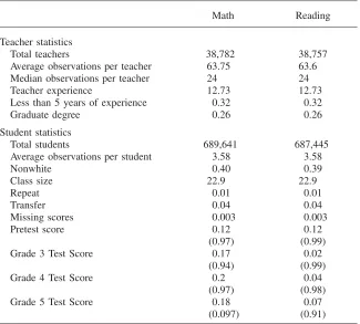
after a few iterations I reach a sample that satisfies the teacher restrictions. I create separate samples, one for math test-score outcomes, and one for reading test-score outcomes. After imposing all the above restrictions, I am left with a sample of approximately 700,000 students, 40,000 teachers, and 2.5 million test-score obser-vations. Close to three-quarters of the entire universe of students who ever attend third through fifth grade between 1998 and 2007 are included in the sample. Notice that students average more than three test-score observations across Grades 3 though 5. This reflects the fact that at the start of Grade 3, students take a pretest in both math and reading. I treat this pretest as an unbiased measure of student ability that is unaffected by prior teacher or other school inputs.25
24. After eliminating a set of teachers, students with fewer than two observations and students who have incomplete teacher histories are eliminated. An incomplete teacher history is problematic for estimating the impact of the contemporaneous teacher since it is not possible to account for the influence of all previous teachers. Note that if a student is simply missing a past test score this is not a problem since I can still account for the lasting impact of the teacher associated with the missing score.
Table 3
Summary Statistics: North Carolina Elementary Students and Teacher
Math Reading
Teacher statistics
Total teachers 38,782 38,757
Average observations per teacher 63.75 63.6
Median observations per teacher 24 24
Teacher experience 12.73 12.73
Less than 5 years of experience 0.32 0.32
Graduate degree 0.26 0.26
Student statistics
Total students 689,641 687,445
Average observations per student 3.58 3.58
Nonwhite 0.40 0.39
Class size 22.9 22.9
Repeat 0.01 0.01
Transfer 0.04 0.04
Missing scores 0.003 0.003
Pretest score 0.12 0.12
(0.97) (0.99)
Grade 3 Test Score 0.17 0.02
(0.94) (0.99)
Grade 4 Test Score 0.2 0.04
(0.97) (0.98)
Grade 5 Test Score 0.18 0.07
(0.097) (0.91)
Note: Sample is constructed using cohorts of North Carolina third grade students who enter between 1998 and 2005. Sample selection is discussed in Section IV. Overall, close to three-quarters of the entire universe of students who ever attend third through fifth grade between 1998 and 2007 are included. Math and reading end-of-grade exams are available at the end of third, fourth, and fifth grade. In addition, a pretest score is available from the beginning of third grade. Scores are normalized using the means and standard deviations of test scores in standard setting years as suggested by the North Carolina Department of Instruction. Observations per Teacher indicate the number of student test scores associated with a particular teacher. Graduate degree is an indicator that a teacher received any advanced degree. Repeat is an indicator that a student is repeating the current grade. Transfers indicate that the student is new to the current school.
percent of the sample. There are very few transfers, missing scores, or repeaters. Close to 67 percent of the sample progresses through Grades 3 though 5 without missing any test scores, moving out of the state, switching to a charter school, or switching to a school without self-contained classrooms.
The test scores in third, fourth, and fifth grade come from state mandated end-of-grade exams. The scores are normalized using the means and standard deviations of test scores in standard setting years as suggested by the North Carolina Department of Instruction.26Because both the math and reading exams changed during the time
frame, the normalizations vary according to the year of the exam. As an example, the first standards setting year is 1997 for both reading and math. In 2001, a new math exam was put in place, making 2001 the new standard. Thus from 1997–2000, all test scores are normalized using the means and standard deviations in 1997. This allows for test scores to improve over time either because students or teachers are improving. Ideally, the method should be employed using a vertically scaled test that remains consistent over time. Overall, the mean test scores are slightly positive, suggesting that even with the limited amount of data cleaning students are still positively selected. The fact that student performance appears to have improved over time also results in positive test-score means.
As Section II illustrates, the amount of teacher and student sorting across schools and classrooms can have important implications for estimates of teacher quality. To provide a sense for the type of sorting in North Carolina’s primary schools, I examine the dispersion in student test scores at the population, school, and teacher level in Table 4. In addition to examining the dispersion in contemporaneous scores, I also look at the dispersion in lag scores and pretest scores based on the third, fourth, and fifth grade classroom assignments.
Table 4 illustrates that there exists significant sorting at the school and classroom level, regardless of whether the contemporaneous, lag, or pretest score is considered. The fact that contemporaneous outcomes vary less and less as we move from the population to the classroom suggests that students are sorted by ability into schools and classes, and that teacher quality likely varies significantly across classrooms. The model with student and teacher effects will help disentangle these two com-ponents. The data is also generally consistent with the notion that there is limited sorting on lagged student outcomes. Note that the ratio of the within teacher variation to the within school variation in lag scores is very similar across third, fourth, and fifth grade. However, the lag score in third grade, which is actually the pretest score, is not observed at the time third grade teachers are assigned. As a result, the sorting into third grade teacher assignments likely reflects sorting on unobserved student ability. In addition, the magnitude of the within teacher sorting based on pretest scores in fourth and fifth grade is quite similar to the sorting based on lag-scores. This result is not consistent with a process that has principals assigning teachers based strictly on test-score outcomes in the previous grade.
V. Results
Using the North Carolina public school data, I estimate multiple ver-sions of the cumulative model of student achievement. I start with the baseline
The
Journal
of
Human
[image:23.432.74.594.110.311.2]Resources
Table 4
Evidence of Student and Teacher Sorting in NC
Math Reading
Within- Within- Within- Within-Population School Teacher Population School Teacher
Third Grade School/Teacher Assignments
Standard deviation third grade score 0.913 0.857 0.817 0.957 0.907 0.881 Standard deviation lag score 0.952 0.897 0.868 0.980 0.937 0.910
Fourth Grade School/Teacher Assignments
Standard deviation fourth grade score 0.959 0.898 0.851 0.960 0.905 0.878 Standard deviation lag score 0.904 0.847 0.815 0.944 0.893 0.868 Standard deviation pretest score 0.945 0.891 0.857 0.975 0.932 0.901
Fifth Grade School/Teacher Assignments
Standard deviation fifth grade score 0.961 0.894 0.853 0.887 0.834 0.807 Standard deviation lag score 0.953 0.894 0.858 0.950 0.895 0.870 Standard deviation pretest score 0.942 0.889 0.854 0.972 0.930 0.898
version which assumes a constant geometric decay rate and time-invariant teacher and student ability. The results from this simple accumulation model are then con-trasted with the results obtained utilizing the levels and growth frameworks. Finally, I estimate more flexible accumulation models that provide greater insight into the true underlying production of student achievement.
A. Baseline
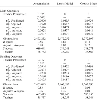
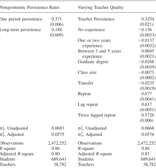
Table 5 presents estimates from the baseline accumulation model, the levels speci-fication, and the growth specification for math and reading scores. The results in-dicate that in both math and reading, teacher effects persists at a rate that is neither 0 or 1. Teacher effects persist at a rate equal to 0.38 for math outcomes and 0.32 for reading outcomes. These results fall in the range of previous estimates of the decay rate discussed in the introduction.
The overall dispersion in teacher quality is estimated to be quite significant for math outcomes, and somewhat smaller for reading outcomes. A one standard devi-ation increase in contemporaneous teacher quality increases math (reading) test scores by approximately 0.25 (0.14) of a standard deviation of the test-score distri-bution. These results are larger than previous estimates, partly because I do not include school effects.27Including school effects in the baseline model indicates that
a one standard deviation increase in teacher quality increases math scores by only 0.2 of a standard deviation of the test-score distribution. This effect is identified only from variation in teacher quality within each school-grade combination. The persistence parameter is unchanged when school effects are incorporated.
The final two columns in Table 5 provide estimates of the dispersion in teacher quality under the assumptions that teacher inputs do not persist at all, or perfectly persist. They are included to illustrate the importance of modeling student achieve-ment as a cumulative process. For math outcomes, the overall importance of teacher quality is understated in the levels framework and overstated in the growth frame-work. For reading outcomes, the levels and growth models result in upward-biased estimates of teacher dispersion, however, the differences are quite small. As a result, in the following discussion I focus on the results for math outcomes only.
The result that the overall dispersion in teacher quality is biased downward in the levels model and biased upward in the growth model is a result of the fact that teacher quality is only slightly positively correlated across grades. The unadjusted cross-grade correlation in teacher quality is approximately 0.11, with a slightly smaller correlation between third and fourth grade teachers, and a slightly larger correlation between fourth and fifth grades. Table 1 illustrates that for very low
Table 5
Estimates of Baseline Accumulation, Levels, and Growth Models Using NC Data
Accumulation Levels Model Growth Model Math Outcomes
Teacher Persistence 0.375 0 1
(0.007) — —
Unadjusted
2
σT, 0.0676 0.0635 0.0726
Adjusted
2
σT, 0.0570 0.0547 0.0607
Adjusted
2
σTj3, 0.0546 0.0459 0.0550
Adjusted
2
σTj4, 0.0628 0.0577 0.0648
Adjusted
2
σTj5, 0.0507 0.0601 0.0536
Observations 2,472,252 2,472,252 1,772,197
R-square 0.86 0.86 0.14
AdjustedR-square 0.80 0.80 0.12
Students 689,641 689,641 688,573
Teachers 38,782 38,782 38,567
Reading Outcomes
Teacher Persistence 0.317 0 1
0.016 — —
Unadjusted
2
σT, 0.0344 0.0322 0.0380
Adjusted
2
σT, 0.0204 0.0207 0.0219
Adjusted
2
σTj3, 0.0288 0.0233 0.0305
Adjusted
2
σTj4, 0.0180 0.0196 0.0157
Adjusted
2
σTj5, 0.0125 0.0187 0.0112
Observations 2,463,093 2,463,093 1,762,790
R-square 0.83 0.83 0.06
AdjustedR-square 0.76 0.76 0.04
Students 687,445 687,445 686,055
Teachers 38,757 38,757 38,544
Note: Sample is constructed using cohorts of North Carolina third grade students who enter between 1998 and 2005. Samp