Simen Markussen and Knut Røed are senior research fellows at the Ragnar Frisch Centre for Economic Research. This paper is part of the project “Social Insurance and Labor Market Inclusion in Norway,” funded by the Norwegian Research Council (grant #202513). Thanks to Bernt Bratsberg, Oddbjørn Raaum, and three anonymous referees for valuable comments. The administrative microdata used in this paper were received from Statistics Norway by consent of the Norwegian Data Inspectorate. The authors are not in a position to make the data available to other users, but Statistics Norway can provide access subject to approval of an application. Interested Norwegian scholars may consult www.ssb.no / mikrodata / . Access from outside Norway is restricted. Statistics Norway may allow access, however, via statistical agencies in the country in question, provided they operate with suffi cient guarantees of confi dentiality. The authors of this paper will help scholars seeking access to these data as best they can. Correspondence to: Knut Røed, the Ragnar Frisch Centre for Economic Research, Gaustadalléen 21, 0349 Oslo, Norway. email: knut. roed@frisch.uio.no.
[Submitted September 2012; accepted February 2014]
ISSN 0022- 166X E- ISSN 1548- 8004 © 2015 by the Board of Regents of the University of Wisconsin System
T H E J O U R N A L O F H U M A N R E S O U R C E S • 50 • 4
Simen Markussen
Knut Røed
Markussen and RøedABSTRACT
Based on administrative panel data from Norway, we examine how social insurance claims spread among neighbors and former schoolmates. We use a fi xed effects methodology that accounts for endogenous group formation, contextual interactions generated by predetermined social factors, and time- constant as well as time- varying confounders. We report evidence that social insurance claims are contagious. There are signifi cant local peer effects both in the overall use of social insurance and in the propensity to use one particular social insurance program rather than another. The magnitudes of the estimated peer effects rise consistently with measures of geographical and relational closeness.
I. Introduction
(2010); and Eugster et al.(2011). Although far from offering a complete explanation, these empirical patterns may be easier to understand if SI claim propensities exhibit path- dependency due to peer effects; see, for example, Bertrand, Luttmer, and Mul-lainathan (2000) and Durlauf (2004). Such peer effects could result from transmission of work norms or changes in the stigma attached to social insurance claims (Moffi tt 1983; Lindbeck 1995; Lindbeck, Nyberg, and Weibull 1999, 2003), or they could arise from the transfer of information about eligibility rules, application procedures, and ac-ceptance probabilities (Aizer and Currie 2004), or about job opportunities (Ioannides and Loury 2004).
While social interaction effects have been extensively analyzed from a theoretical perspective, empirical analysis has been held back by methodological diffi culties and lack of appropriate data. The fundamental empirical challenge is to disentangle endog-enous interaction from other sources of correlation between individual and group be-havior, such as endogenous group formation and unobserved confounders; see Manski (1993). As shown by our brief literature review in the next section, the existing empiri-cal evidence on SI contagion is scant and, with a few important exceptions, limited to ethnic minorities. Existing evidence is also confi ned to very specifi c SI programs, making it diffi cult to assess whether it has captured peer effects in overall SI depen-dency or in the tendepen-dency to use one specifi c SI program rather than another. The policy implications following from these two competing interpretations are clearly different. In the present paper, we examine social interaction effects within different kinds of networks—or peer groups—that is, neighbors, schoolmates, and ethnic minori-ties. The key research question we ask is whether—and to what extent—an agent’s likelihood of claiming any form of tax- fi nanced income support is causally affected by the level of claims recorded within the various types of networks the agent relates to, conditional on the claim patterns prevailing elsewhere in the economy. In addition, we examine peer effects in the propensity to use one type of SI program rather than another. The question of interest here is whether—and to what extent—the distribu-tion of SI claims between “disability- related” and “unemployment- related” programs within a network affect the group members’ propensities to claim benefi ts from these program types.
We use an extraordinarily rich and detailed panel data set from Norway, covering the whole working- age population over age 17. We exploit the richness of the data to set up empirical models in which we control for the various confounding and sorting problems that often undermine the credibility of reported social interaction effects. In contrast to much of the existing literature, we do not rely on either instrumental variables or movements between networks but instead use individual fi xed effects to remove the infl uence of time- invariant confounders and contextual interactions generated by predetermined social factors, and fl exible time functions to control for network- specifi c shocks and sorting problems that are not eliminated by the individual
relational closeness. For example, we fi nd that an exogenous change in average SI claims within a group of adults who at some time went to the same junior high school together generates cumulative knock- on effects amounting to around 25 percent of the initial change. But, adjusted for group size, the peer effect is much larger among same- level- same- sex schoolmates than it is among more “distant” schoolmates. Within small neighborhoods, we fi nd that an exogenous change in SI claims entails additional knock- on effects amounting to 17 percent of the initial change. Again, the effect is much larger among similar than among dissimilar neighbors and also larger among geographically close than among geographically more distant neighbors. We
fi nd particularly strong interaction effects within ethnic networks, defi ned as im-migrants from a common low- income source country who reside in the same local area. The cumulative peer effect for these groups is estimated to around 38 percent. The peer effects do not cross ethnic boundaries, however; a rise in SI dependency among immigrants from other low- income countries in the same local area has no effect at all.
Our results also indicate considerable scope for substitution between different SI programs. When we distinguish between “disability- related” and “unemployment- related” SI claims, we fi nd that an exogenous rise in a peer group’s use of one of these program types has a much larger effect on group member’s same- type- claims than it has on their overall use of SI. A signifi cant part of the additional SI claims is thus offset by a reduction in claims of the other type. An important implication of this
fi nding is that empirical approaches focusing on a single program only will tend to exaggerate the peer effects in overall SI dependency. Peer effects are important both for the overall level of SI claims and for the allocation of claims across SI programs.
Finally, we show that peers affect SI claim propensities among previous nonclaim-ants (the entry decisions) as well as among more experienced claimnonclaim-ants (the con-tinuation decisions). This suggests that the peer- effects not only mirror a process of information sharing but also impacts on the utility associated with being in a state of benefi t recipiency. And while peers’ use of competing (other- type) SI programs has a negative (substitution) effect on entry into each program type, it has a positive impact on continuation. We conclude from this that the peer effects identifi ed in this paper to a large extent refl ect the propagation of work- norms or the stigma associated with being an SI claimant.
II. Related Literature
heterogeneity (confounding factors); and (3) to deal with the presence of endogenous formation of the groups that act as carriers of social interactions.
There is also a growing empirical literature on peer effects in the utilization of public transfers. Bertrand, Luttmer, and Mullainathan (2000) examines the role of welfare participation within local networks in the United States, defi ned by language spoken. Its empirical strategy is to investigate whether belonging to a language group with high welfare use has larger effects on own welfare use the more a person is sur-rounded by people speaking one’s own language. It fi nds that this is indeed the case and concludes that networks are important for welfare participation. Aizer and Currie (2004) uses a similar approach to study network effects in the utilization of publicly funded prenatal care in California with groups defi ned by race / ethnicity and neighbor-hoods. It concludes that group behavior does affect individual behavior. Furthermore, it shows that the identifi ed network effects cannot be explained by information sharing because the effects persist even for women who had used the program before. Conley and Topa (2002) examines the spatial patterns of unemployment in Chicago and fi nds that local variations are consistent with network effects operating along the dimen-sions of race and geographical and occupational proximity.
The recent literature also includes a number of studies outside the United States. Stutzer and Lalive (2004) examines the pattern of unemployment duration in Swit-zerland and fi nds that strong local work norms—as measured by voting behavior in a referendum on the level of unemployment insurance—tend to coincide with short unemployment durations. Hesselius, Nilsson, and Johansson (2009) uses ex-perimental data from Sweden to examine the extent to which coworkers affect each other’s use of sick pay. The experiment it uses implied that a randomly selected group of workers was subject to more liberal rules regarding the need for obtaining a physician’s certifi cate to prove that their absence from work was really caused by sickness. Hesselius, Nilsson, and Johansson (2009) shows that the reform caused absenteeism to rise both among the treated and the nontreated workers and that the latter effect was larger the larger was the fraction of treated workers at the work-place. Peer effects in absenteeism are also examined by Ichino and Maggi (2000). Its empirical strategy is to study how workers who move between branches in a large Italian bank adapt to the prevailing absence cultures in the destination branches. The key fi nding is that workers adjust own absence behavior in response to the absence level among their new colleagues. A similar approach has been used by Bradley, Green, and Leeves (2007) to study absenteeism among school teachers in Queensland, Australia. Again, the fi nding is that the absenteeism of movers to some extent adapts to the prevailing absence culture at their new school. Åslund and Fredriksson (2009) examines peer effects in welfare use among refugees in Sweden, exploiting a refugee placement policy that generates the rarity of exogenous varia-tion in peer group composivaria-tion. A key fi nding of the paper is that long- term welfare dependency among refugees is indeed higher the more welfare dependent the com-munity is in the fi rst place.
variables strategy. Its key idea is that since the probability of disability program entry in Norway has been shown to be strongly affected by job loss (Rege, Telle, and Votruba 2009; Bratsberg, Fevang, and Røed 2013), exogenous events of layoff in a person’s neighborhood—for example caused by fi rm closure—can be used to instrument the neighbors’ disability program participation (with proper controls for local variations in labor demand). Based on this strategy, Rege, Telle, and Votruba (2012) estimates a sizable network effect implying that a one percentage point ex-ogenous increase in similarly aged neighbors’ disability program participation rate generates an additional increase of 0.3–0.4 percentage points as a result of network effects. Bratberg, Nilsen, and Vaage (2012) and Dahl, Kostøl, and Mogstad (2013) both assess the transmission of disability pension recipiency within families but with completely different empirical strategies. Bratberg, Nilsen, and Vaage (2012) takes the view that the intergenerational transmission of, say, work norms, operates through “exposure,” and identifi es the social interaction effect by comparing siblings who, due to differences in age, to varying extents shared household with their parent after the disability pension was granted. Its fi nding confi rms that longer exposure to a parent claiming disability insurance indeed raises the probability that the offspring also claims such benefi ts later on. Dahl, Kostøl, and Mogstad (2013), on the other hand, mainly focuses on children who were adults at the time of a parent’s potential entry to the disability insurance program and uses a random assignment component in the decision process—the assignment of judges to applicants whose cases were initially denied—as the source of identifi cation of the intergenerational transmission mechanism. Again, the key fi nding is that a parent’s entry to the disability insur-ance program signifi cantly raises the probability that their offspring also enter the program.
What all the pieces of of Norwegian evidence have in common is that they mostly focus on the transmission of permanent disability insurance claims. We will argue that this is an unfortunate limitation because permanent disability insurance typically either substitutes for or is preceded by other social insurance programs, such as sick pay, temporary disability insurance (medical or vocational rehabilitation benefi ts), unemployment benefi ts, or social assistance (welfare). A considerable degree of sub-stitutability between unemployment and disability insurances has been established in several empirical papers; see, for example, Black, Daniel, and Sanders (2002); Autor and Duggan (2003); Rege, Telle, and Votruba (2009); and Bratsberg, Fevang, and Røed (2013). Peer effects may thus be relevant both for the overall SI claim propensity and for the distribution of claims across programs. By focusing on a single program only, it is impossible to distinguish peer effects on the overall use of social insurance from peer effects on the propensity to use one particular program rather than another.
focusing on the observed timing of SI claimsrather than on their occurrence. This approach is backed up by the use of extraordinarily fl exible control functions—with up to as much as 623,000 time- varying dummy variables—arguably eliminating the infl uence of conceivable time- varying confounding factors.
III. Theoretical Considerations
Social interaction models start from the idea that the preferences of individuals over alternative courses of action depend directly on the actions taken by other individuals to whom the individuals relate; see, for example, Brock and Durlauf (2000) and Cont and Löwe (2010) for overviews. The purpose of these models is typically to characterize or to provide an explanation for group behavior that emerges from interdependencies between individuals. To illustrate, let ai indicate individual i’s use of social insurance, and assume that the payoff function associated with this action can be decomposed into a sum of a private and a social component. Let a
i 0
denote the optimal choice in the absence of social interaction and let j∈J be the set of agents that
i relates to. With quadratic utility, we can write
(1) Ui(ai;{aj,j ≠i})=−(ai0−ai)2− ∑j≠i␥ij(ai−aj)2,
with the optimal SI claim characterized by
(2) a*i=
1
+∑j≠i␥ij
(ai0+∑
j≠i␥ijaj).
In this specifi cation, π refl ects the marginal disutility of deviating from the private optimum and γij measures the marginal gain in i’s utilityof conforming to the action of j. Note that it is the actual behavior of j that i conforms to and not the norms / at-titudes that motivate j’s behavior. Hence, γij represents what Manski (1993) refers to as endogenous interaction. While endogenous and contextual interactions both rep-resent important social propagation mechanisms, it may be important from a policy perspective to discriminate between them as only endogenous interactions are able to create spillover or multiplier effects of policy interventions targeted at changing actual behavior. Formally, endogenous interactions imply that optimal choices are determined in a large simultaneous equations system with as many equations as there are individuals.
We emphasize that SI contagion in this context does not necessarily refl ect the prevalence of fraudulent claims. Both unemployment- related and disability- related SI programs involve substantial scope for subjective judgment with respect to whether a given health or unemployment problem is suffi ciently serious to justify benefi ts, and there is also considerable overlap between different programs. In addition, individuals can obviously exert more or less effort in order to prevent the need for SI to arise in the
fi rst place as well as to escape from it. Hence, even in cases with strict screening and monitoring (for example, in the form of physician certifi cation or job- search require-ments), the utility (or disutility) associated with different types of benefi t- recipiency matters for the realized level of claims.
different ways. For example, the choice γij = γ / N, where N is the size of the popula-tion (excluding i), leads to the global interaction model, where each agent’s prefer-ences are affected by the average action of all others, as in Lindbeck, Nyberg, and Weibull(1999) and Glaeser, Sacredote, and Scheinkman (2003). By contrast, local interaction models assume that social infl uences are mediated within confi ned groups, potentially differentiated by some notion of “distance” such that γij = γ(dij), where dij
is a measure of relational distance between i and j. Studies on the structure of social groups show that individuals tend to interact most with other individuals who are similar to themselves; see, for example, Marsden (1982). In empirical applications, social interactions are thus typically assumed to take place within peer groups defi ned in terms of such factors as neighborhoods, workplaces, school classes, families, or races—often in combination with demographic factors (gender, age) and measures of “social distance” (for example, educational attainment or “class”).
In the present paper, we focus on local interactions. Interaction effects are exam-ined at group levels, and group averages are used as the central explanatory vari-ables. This implies that the bivariate interaction effects—the direct infl uence of one person on another—are modeled as homogeneous within (narrowly defi ned) groups and inversely related to group size—that is, γij = γg / Ng, where g denotes the group in question and Ng is the number of group members apart from i. An important as-sumption embedded in this framework is that average distance increases with group size, ceteris paribus, such that the larger the number of peers in a particular group, the smaller the infl uence exercised by each and one of them. Equation 2 can then be reformulated as
(3) ai*= 1
+∑g␥g
(ai0+∑
g␥gag,−i),
where γg is the utility of conforming to the average behavior in group g (ag,−i). This parameter clearly depends on the weight attributed by individual i to the behavior of group g, which is again a refl ection of its relational closeness and potentially also its size. We typically expect γg≥ 0, but γg < 0 can of course not be ruled out. Negative interaction effects may occur when agents derive utility from displaying novelty, as in fashion and fads, or from signaling a distance to groups with which one does not wish to be associated.
IV. Institutional Setting and Data
The Norwegian public system of social insurance is comprehensive. In the present paper, we examine all the major social insurance programs relevant for the working age population in Norway; that is:
• Unemployment insurance
• Sick- pay (spells exceeding 16 days only)
• Temporary disability insurance (including medical and vocational rehabilitation) • Permanent disability insurance
Entitlement to unemployment insurance, sick leave benefi ts, and subsidized early retirement is obtained through regular employment, whereas rehabilitation benefi ts, disability pension, and social assistance in principle can be obtained without such experience. The replacement ratios for unemployment insurance, temporary and manent disability, and subsidized early retirement all typically lie around 60–65 per-cent of previous earnings but with minimum and maximum levels. For sick leave, the replacement ratio is 100 percent, but these benefi ts can only be maintained for one year (persons who are still unable to work after one year of sickness can apply for tem-porary or permanent disability benefi ts). All disability- related benefi ts, including sick pay, need to be certifi ed by a physician. Yet, in practice it has turned out to be diffi cult for physicians to “overrule” their clients’ own judgments; see Markussen, Røed, and Røgeberg (2013). Social assistance constitutes the last layer of social insurance and is primarily targeted at individuals with no other income sources. In contrast to the other benefi ts, it is means tested against family income.1
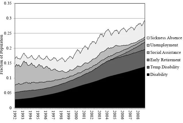
Our data cover social insurance claims for the whole Norwegian population from 1992 through 2008. Because we have chosen to use a balanced panel (see next sec-tion), we limit the analysis to individuals who were between 18 and 66 years through-out this period, implying that they were born between 1942 and 1974. This implies that our analysis comprises 33 complete birth cohorts, conditioned on being alive and residing in Norway in 1992–2008. Figure 1 gives an overview of these cohorts’ social insurance claims—month by month—by SI program. Our primary interest does not lie in the use of each particular program, however, but rather in overall SI claims. This focus is partly motivated by the fact that the distinction between the different programs is blurred (Bratsberg, Fevang, and Røed 2013), with large fl ows between them (Fevang et al. 2004), and partly by our ambition to identify patterns of interest beyond a narrow program- specifi c Norwegian setting. We are also not particularly interested in the high- frequency (month- to- month) fl uctuations in SI use, which for some of the programs are dominated by seasonal factors. Hence, in the main part of our statistical analysis, we aggregate the observed social insurance outcomes into an annual dependent variable measuring the number of months with benefi t claims from any of the social insurance programs in Norway.2 However, to illuminate how
peers potentially affect the selection of particular SI programs, we also set up mod-els where we distinguish the presumed disability- related programs (sick pay, tempo-rary and permanent disability benefi ts, early retirement benefi ts) from the presumed unemployment- related programs (unemployment benefi ts, social assistance).
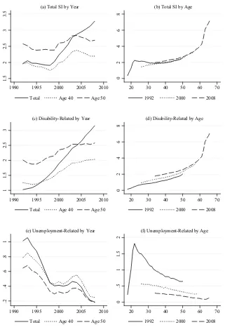
Figure 2 illustrates some key descriptive features of the dependent variables that we are going to use in the empirical analysis. The two upper panels show how the overall use of SI developed within our analysis population from 1992 through 2008, by year and age, respectively. Since we follow the same group of people over time in this analysis, it is clear that the strong age gradient shown in Panel b is an important factor behind the observed trend in social insurance claims shown in Panel a. This is also illustrated by the much weaker time trend observed in Panel a when the age
1. Due to space considerations, we do not give a detailed description of Norwegian social insurance institu-tions here. More thorough descripinstitu-tions (in English) are provided by Halvorsen and Stjernø (2008) and by the European Commission (2011).
level is fi xed (at age 40 and age 50, respectively). It still seems to be the case, though, that the overall SI caseloads rose signifi cantly in the period from around 1993–2003, after which there was a small decline. The four lower panels illustrate the corre-sponding developments for disability- related and unemployment- related SI claims separately. They reveal a sharp increase in disability- related claims and a decline in unemployment- related claims.
The important role that age seems to play in the determination of individual SI claims suggests that the social interaction effects generated by a given average SI use among peers may depend on the age composition of the peer group in question. For example, a high SI rate primarily caused by a large fraction of elderly individuals in the peer group may have a different impact on work morale than the same high rate caused by unusually high claimant rates among younger individuals. We will there-fore use age- adjusted peer group averages in the statistical analyses; that is, for each person- year in the peer group, we subtract the grand (national) age- specifi c mean for the year in question and then add the corresponding mean for 40- year- olds. As a result, we obtain age- adjusted observations normalized to a person aged 40.
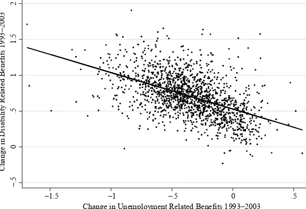
During the period of declining unemployment and rising disability- related SI claims in the 1990s, an interesting cross- sectional pattern emerged whereby the local rises in disability- related claims tended to be larger the steeper were the declines in unemployment- related claims. This is illustrated in Figure 3, where for 1,535 local areas in Norway (to be described in the next section) we plot the changes in average age- adjusted disability claims from 1993 to 2003 against the corresponding changes
0 0.05 0.1 0.15 0.2 0.25 0.3 0.35
1992 1993 1994 1995 1996 1997 1998 1999 2000 2001 2002 2003 2004 2005 2006 2007 2008
F
ra
ct
ion of P
opul
at
ion
Sickness Absence
Unemployment
Social Assistance
Early Retirement
Temp.Disability
Disability
Figure 1
Social Insurance Claims for the 1942–1974 Birth Cohorts from 1992.1 to 2008.12
1.
Number of Months with SI Claims in Norway, by Year (1992–2008) and Age (18–66)
in unemployment- related claims. The marked inverse relationship between these local trends raises the question of whether a causal relationship exists. One potential source of such a relationship could be program substitution generated by “cross- program” peer effects. For example, it is conceivable that in areas with a particularly sharp decline in unemployment due to a booming labor demand, it became less attractive to present a given “labor market problem” as being caused by unemployment and more attractive to present it as being caused by poor health.
V. Empirical Analysis
In this section, we set up linear regression models designed to fi nd out whether—and to what extent—an individual’s use of social insurance benefi ts is caus-ally affected by the (age- adjusted) use within networks / groups to which the individual is closely—or more vaguely—attached. Our primary dependent variable is going to be a person- year observation reporting the number of months with SI claims, either in total or for disability- and unemployment- related programs separately. The key ex-planatory variables are the following: (1) a person- fi xed effect; (2) the individual’s own claim last year; (3) the average claims among peers last year; and (4) a vector of group- year fi xed effects, where—essentially —the grouping does not coincide exactly
–.5
Mean changes calculated for all local areas with at least 100 inhabitants
Figure 3
Changes in Age- Adjusted Social Insurance (SI) Claims in 1,535 Local Areas in Norway
with the peer groups. In some specifi cations, we also use observed time- varying vari-ables defi ned at the peer- group level to account for possible confounders.
To circumvent the problem of dynamic endogenous group formation, we focus throughout this paper on groups that—by defi nition—are stable; that is, former schoolmates and persons that resided in the same geographical area at the start of our observation period. The price we pay for this is that our “networks” will serve as imperfect proxies for the various groups of people with whom agents actually interact. Hence, compared to analyses based on positively identifi ed and closely tied networks, we expect that interaction effects identifi ed in our analysis will be signifi cantly at-tenuated.
We fi rst present the model for total SI claims. Let yi,t be the number of months that individual i claimed (any form of) SI benefi t in year t and let yg,−i,tbe the correspond-ing age- adjusted SI propensity (see previous section) for persons belongcorrespond-ing to a group
g in year t, excluding individual i. We set up fi xed effects models of the following form:
(4) yi,t = ␣i+yi,t−1+ht(xi)+∑g∈Ggyg,−i,t−1+uit,
where ␣i is an individual fi xed effect, ht(xi) is a time function specifi ed separately for
different combinations of individual covariates xi, and G is the set of groups / networks potentially infl uencing the behavior of i. The parameters of main interest are the θg’s, which refl ect the fi rst- year peer effects. There will also be knock- on effects in subse-quent years, as the fi rst- year effect propagates both through the autoregressive process and through additional higher- order peer effects. The knock- on effects will decline over time provided that (θg + ρ) < 1. Consider an exogenous and transitory shock in
group g’s SI dependency of size z. Next year, this shock implies a change in SI depen-dency equal to (θg + ρ)z, and the year after that (θg + ρ)2z and so on. Hence, the
cumu-lative knock- on effects arising from the shock amounts to z[(g+)+(g+)2+…], which converges toward z(θg + ρ)(1 – θg – ρ)–1. Without peer effects, it would instead
converge toward zρ(1 – ρ)–1. Hence, as a measure of the total cumulativepeer effect,
we compute the statistic
(5) g = g+ 1−g−−
1−,
which represents the total number of extra SI months—over and above what arises from the autoregressive process alone—that accrues in response to a one- year transi-tory shock in the group average due to the peer effects.
The individual fi xed effect (αi) is included in Equation 4 to control for sorting on overall SI- propensity into networks, for time- constant confounders, and for prede-termined contextual sources of interaction. It ensures that it is the timing—not the occurrence—of SI claims within networks that identifi es the effects of interest. At fi rst sight, it may appear unnecessary to use individual fi xed effects in this setting because it is disturbing factors at the network level that we primarily worry about. However, without individual fi xed effects, we could not have justifi ed the critical assumption of exogenous peer behavior in year t–1as it would have been affected by individual i’s own (unaccounted for) SI propensity in earlier years.
simultaneity problem because a person’s past SI statuses (more than one year ago) will have had a causal impact on the peers’ SI statuses last year and at the same time be correlated with the individuals’ SI propensities this year.
Individual time functions ht(xi) are included to control for time- varying confounding factors with a geographical and / or individual dimension. They are modeled as large numbers of group- specifi c time- varying dummy variables, for example, in the form of separate time- dummies for each travel- to- work area or for each neighborhood in Nor-way, and / or separate time- dummies for groups defi ned by combinations of birth year, gender, and educational attainment. In some cases, they also include directly observed covariates, for example, in the form of indicators for local labor market fl uctuations. Their specifi c formulations vary across different models (as will be explained below), but they are defi ned on the basis of persons’ initial characteristics. In the main part of our analysis, we do not exploit information on, for example, migration or additional educational attainment during our observation period as we expect that such events to some extent are endogenous responses to changes in labor market status (including transitions to social insurance dependency).
Note that although this setup disentangles endogenous interactions from predeter-mined contextual effects, for example, related to within- peer- group- correlations in values, preferences, and abilities, it cannot fully separate endogenous interactions from time- varying contextual effects. For example, if for some reason an exogenous change in norms / attitudes occurs within a peer- group, this may result in a correspond-ing change in the affected individuals’ observed SI use. We will then not be able to say with certainty whether the subsequently identifi ed contamination effects represent en-dogenous interactions (that is, are caused by the peers’ actual use of SI) or contextual interactions (that is, are caused by the peers’ changed norms / attitudes).
To estimate Equation 4, we use a fi xed effect “within- estimator” that centers the model along several dimensions and thus avoids estimating parameters that are not of direct interest to us.3 As a consequence, the model eventually estimated by OLS
con-tains a residual that incorporates a covariate- adjusted individual mean (over all years), and is thus not completely exogenous with respect to the lagged dependent variable (see, for example, Cameron and Trivedi 2005, p. 764). Consistency requires that the average residual is small relative to each period’s residual, which again requires that the number of time periods is large. To assess the potential bias in our case, we have, as part of a series of robustness exercises, also estimated Equation 4 with an instru-mental variable (2SLS) technique proposed by Anderson and Hsiao (1981). We then rely on fi rst- differencing (instead of mean- centering) to get rid of the person- fi xed effect, and instrument the resultant lagged differences {(yi,t–1 – yi,t–2), (yg,−i,t−1−yg,−i,t−2)} with their second lag levels {yi,t−2,yg,−i,t−2}.4 As we show below, it turns out that the fi rst- difference 2SLS estimates of peer effects are somewhat larger than the fi xed ef-fects OLS estimates although the differences are not statistically signifi cant.
3. Due to the large number of observations (up to around 16 million person- years, see next section) and the large number of dummy variables (around 623,000 in the most fl exible specifi cation) in addition to the person- fi xed effects, estimation raises some computational challenges. We have used a novel algorithm based on The Method of Alternating Projections as described in Gaure (2013) and implemented in the R- package “lfe”; see http: // cran.r- project.org / web / packages / lfe / citation.html.
To examine peers’ infl uence on the choice of particular SI program, we also esti-mate models where we distinguish between the disability- related and the unemployment- related programs (see Section IV). Let yiP,t be the number of months
individual i claimed benefi ts of type P (=H(ealth),U(nemployment)) in year t. The statistical models then take the form:
(6) yiP,t = ␣ i P+
UPyiU,t−1+HPyiH,t−1+Pht(xi)
+∑g∈G(UgP yUg,−i,t−1+PHgygH,−i,t−1)+uitP, P= H,U
where (yg,U−i,t,y g,−i,t
H ) are the averages (excluding individual i) in peer group g.
In the next subsections, we fi rst examine interaction effects within three different types of networks separately; that is, neighborhoods, schoolmates, and ethnic minori-ties. We then present a brief assessment of some underlying mechanisms based on separate analyses of SI entry and continuation decisions. In principle, we could have examined all types of networks simultaneously. However, as we explain below, the analysis of each network type requires different cuts and adaptations of the data and the models.
A. Neighbors
We start out examining the impacts of social insurance dependency within residential areas. The purpose is to examine the degree to which SI claim propensities spread endogenously within local communities and to which extent such interaction effects depend on geographical and relational distance. The latter is measured by differences in age, gender, and educational attainment. To avoid endogenous geographical sorting, our analysis is based on recorded address at the start of our analysis period in 1992. To reduce the potential attenuation bias caused by subsequent out- migration, we limit the analysis in this subsection to persons belonging to the 1942- 60 birth cohorts, implying that they were between 32 and 50 years old—and hence reasonably settled—at the time of peer group construction in 1992.5 We also limit the analysis to persons born
in Norway to avoid overlap with a separate analysis of the immigrant population in a later subsection.
We examine peer effects at three geographical levels: neighborhoods, local areas, and municipalities. Our defi nition of neighborhoods corresponds to the so- called “ba-sic statistical units” (“grunnkretser”) used by Statistics Norway. They are designed to resemble genuine neighborhoods and contain residences that are homogeneous with respect to location and type of housing.6 There are 13,700 basic statistical units in
Norway, each populated by around 350 individuals on average. Each neighborhood is part of a somewhat larger “local area.” Given the geographical proximity, we would expect there to be some room for social interaction between residents of neighboring neighborhoodsalthough not to the same extent as for same- neighborhood residents. The local areas correspond to the so- called “statistical tracts” (“delområder”) drawn
5. In our data, 58 percent of the individuals lived in exactly the same neighborhood in 2008 as they did in 1992.
up by Statistics Norway. They are designed to encompass neighborhoods that naturally interact, for example, by sharing common service / shopping center facilities. A typical local area comprises around eight to nine neighborhoods and 3,100 inhabitants. Local areas are again part of municipalities. It is likely that there is some interaction be-tween people living in different local areas in the same municipality also but less than between people living in the same neighborhood or local area. A typical municipality consists of three to four local areas and 11,700 inhabitants.
It follows that we would expect genuine peer effects to be stronger within neigh-borhoods than within local areas and stronger within local areas than within munici-palities. To ensure that the peer groups in local areas and municipalities are directly comparable to those in the neighborhood, in terms of size as well as composition, we construct them artifi cially by conducting a one- to- one exact- match sampling; that is, for each person in i’s own neighborhood, we draw one person from the local area (outside own neighborhood) and one from the municipality (outside own local area), respectively, who is of the same gender, has the same age (+ / – one year), and has exactly the same education.7 Finally, as part of a placebo analysis, we also assemble a
matched group of “peers” from a different part of the country (defi ned as being from a nonneighboring county).
In total, there are around one million individuals included in this part of the anal-ysis, each of them contributing 16 annual observations (the 1992 observations are lost due the inclusion of the lagged variables); see Table 1. This leaves us with a total number of more than 16 million person- year observations. On average, the persons in our data set claim social insurance benefi ts in around 2.7 months each year.
In a baseline model, the vector of time- varying control variables ht(xi) includes separate year- dummies for each travel- to- work area (TWA) in Norway and separate year- dummies for each combination of birth year, sex, and education (the latter with 15 categories refl ecting both the level and the type of education).8 There are 90 TWAs
in Norway, defi ned by Statistics Norway to ensure that persons living in each of these areas operate in a common labor market and have, thus, been subject to the same geo-graphical fl uctuations in labor market tightness over time. However, to account for the possibility of labor market fl uctuations operating at even lower geographical levels,
ht(xi) also includes indicators for neighborhood- specifi c shocks. More specifi cally, we include an annual downsizing indicator, which is equal to one if at least two persons belonging to the same neighborhood and working in the same fi rm register as unem-ployed in the same year. To account for more general neighborhood- specifi c economic
fl uctuations, we fi rst compute nationwide industry- specifi c annual transition rates from employment to unemployment for all Norwegian employees.9 We then use the initial
(1992) employment structure in each neighborhood to compute neighborhood- specifi c
7. If we fi nd more than one match satisfying these criteria, we draw one of them randomly. If we do not
fi nd matches at all geographical levels, the person in question is dropped from the peer group (7.5 percent of individuals).
8. With this specifi cation, we can obviously not distinguish age from time effects because age and time is perfectly correlated at the individual level; see Biørn et al.(2013).
weights. Finally, we use these weights, multiplied with the nationwide time- varying industry specifi c unemployment risks, to compute a variable representing the annual unemployment risks for each neighborhood.
Even with this fl exible model, we still cannot rule out the occurrence of confound-ing shocks in the form of unaccounted for labor market fl uctuations or of changes in the local SI admittance practices. In robustness exercises, we expand the model to comprise separate year dummies for each of the around 450 social insurance districts, for each of the 1,700 local areas, or for each of the 4,700 family- physician practices in Norway, respectively (instead of the 90 TWAs).10 We also run an additional “placebo”
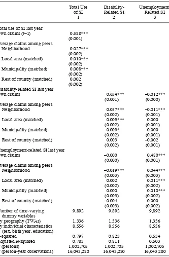
analysis using annual earnings for non- SI claimants as the outcome of interest. Estimation results from a set of baseline models are presented in Table 2. Look-ing fi rst at the total use of SI (regardless of type) in Column 1, we note that there is a signifi cant peer effect associated with neighborhoods estimated to 0.027. With an autoregressive coeffi cient equal to 0.588, this implies a cumulative peer effect (as computed in Equation 5) of around 17 percent. Moving on to the neighboring neigh-borhoods in the local area—while maintaining the size as well as the gender- education- composition of the peer group—the size of the effect is cut by approxi-mately two- thirds; moving even farther away within the municipality, it declines fur-ther. Hence, we identify a clear pattern of declining peer effects as the geographical distance increases. Looking at a matched group of artifi cial peers in another part of the country, the “effect” is approximately equal to zero. As an additional “falsifi cation test,” we have also estimated a model where we include the behavior of the matched peer group in another part of the country as the only peer variable—that is, as a sub-stitute for the true peer groups. We then obtained a similar insignifi cant estimate of –0.001 (standard error 0.002), suggesting that the estimated peer effects in Table 2 do
10. Separate year- dummies for each family- physician group are included to control for possible con-founding factors related to changes in the local physicians’ lenience / strictness with respect to certifying disability- related SI claims. Registers with information of physician- patient- linkages are not available before 2001; hence, we use the 2001 patient lists in this particular exercise. Social insurance districts follow munici-pality borders except in the largest cities, where there are multiple social insurance districts. Persons living in the same neighborhood or local area also belong to the same social insurance district.
Table 1
Descriptive Statistics—Neighborhoods (1942–1960 cohorts)
Number of individuals 1,002,705
Number of neighborhoods 11,828
Average size of the neighborhood (based on observations for individuals) 343.9
Mean annual number of months with SI benefi ts of any kind 2.68
Mean annual number of months with disability- related benefi ts 2.37
Mean annual number of months with unemployment- related benefi ts 0.37
Individuals with 0 benefi t months all years (percent) 18.9
Individuals with 12 benefi t months all years (percent) 5.2
Total Use
Rest of country (matched) 0.002
(0.002)
Local area (matched) 0.009*** 0.000
(0.002) (0.001)
Municipality (matched) 0.009* 0.000
(0.002) (0.001)
Rest of country (matched) 0.003 –0.002
(0.002) (0.001)
Local area (matched) 0.002 0.011***
(0.002) (0.002)
Municipality (matched) 0.000 0.010***
(0.003) (0.002)
Rest of country (matched) –0.004 0.000
(0.003) (0.002)
Adjusted R- squared 0.783 0.811 0.503
N (persons) 1,002,705 1,002,705 1,002,705
N (person- year observations) 16,043,280 16,043,280 16,043,280
not result from unobserved shocks correlated to the gender- age- education- composition of neighborhoods.
Turning to the separate models for disability- related (Column 2) and unemployment- related SI claims (Column 3), we fi nd that the direct (same SI type) peer effects are of similar size or larger than the total peer effects, while there are small, but signifi cant, negative “cross effects.” The latter indicates a considerable scope for substitution be-tween the two types of SI and that peer behavior affects both the overall propensity to claim SI benefi ts and the type of benefi ts actually claimed.
As noted above, the identifi cation of peer effects in this paper rests on the assump-tion that, controlled for time- varying covariates, any remaining shocks in SI claims do not have a spatial pattern that coincides with our peer group defi nitions. While we have argued that it is hard to envisage such confounding shocks, we now examine the validity of the assumption more formally through a number of robustness analyses. In this exercise, we focus exclusively on the neighborhood peer effect on total SI use. Our primary strategy is to examine what happens with the estimated peer effect as we include ever more fl exibility in the time- varying control functions—in the form of shocks at lower geographical levels or in the form of more differentiated geographical shocks. To check the potential bias arising from the correlation between the lagged dependent variable and the residual, we also report estimates from a fi rst- differenced IV (2SLS) model, where the lagged differences are instrumented by their second lag levels.
The results from the robustness analysis are presented in Table 3. As we introduce more fl exibility in the controls for local shocks in Columns 2–5, the estimated neigh-borhood peer effects decline somewhat but remain statistically signifi cant in all
speci-fi cations. A point to bear in mind here is that the most fl exible models entail the risk of “over- controlling,” in the sense that the dummy control vectors absorb some genuine peer effects. It is notable that that the model’s overall explanatory power—as mea-sured by R- squared—is virtually unchanged as separate year dummies are introduced at ever lower geographical levels. For example, substituting 57,526 family- physician year dummies (Column 4) for the 1,336 TWA year dummies (Column 1) raises the unadjusted R- squared from 0.797 to 0.798.
Switching estimation technique from fi xed effects OLS to fi rst- differenced 2SLS does change the estimated peer effect considerably yielding a cumulative effect as high as 0.34; see Column 6. The standard errors also become much larger, however, implying that the cumulative effect is estimated with considerable statistical uncer-tainty. Yet, if anything, the 2SLS results indicate that our within- estimators may un-derestimate the neighborhood effect rather than overestimate it.
dur-M
arkus
se
n a
nd Røe
d
1099
1 2 3 4 5 6
Own claims (t–1) 0.588*** 0.588*** 0.588*** 0.587*** 0.588*** 0.559***
(0.001) (0.001) (0.001) (0.001) (0.001) (0.001)
Average claims among neighbors in own neighborhood
0.027*** 0.021*** 0.015*** 0.018*** 0.026*** 0.057**
(0.002) (0.002) (0.002) (0.002) (0.002) (0.010)
Implied cumulative peer effect 0.170 0.130 0.092 0.110 0.163 0.337
Geographical year dummy variables
TWA 1,336 1,336
Municipality 6,586
Local area 23,131
Physician (in 2001) 57,526
Individual year dummy variables
Gender×education×birth year 8,556 8,556 8,556 8,556 8,550
Interaction of geographical and individual year dummy variables
Gender×education×birth year×TWA 622,996
Estimation method (OLS / 2SLS) OLS OLS OLS OLS OLS 2SLS
R- squared 0.797 0.797 0.798 0.798 0.805 0.795
Adjusted R- squared 0.783 0.783 0.784 0.783 0.783 0.780
N (persons) 1,002,705 1,002,705 1,002,705 992,002 1,002,705 1,002,705
N (person- year observations) 16,043,280 16,043,280 16,043,280 15,872,032 16,043,280 15,861,750
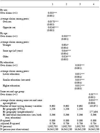
ing our observation period. This is obviously a highly selected group of persons. How-ever, if there are any remaining unaccounted for time- varying confounders related to economic fl uctuations at the neighborhood level, these confounders most likely would affect earnings levels as well as employment levels. Our placebo analysis is based on an individual fi xed effects model where we include exactly the same neighborhood SI peer variable as in the regressions above, and also include year dummies by TWA and by individual characteristics (as in Table 3, Column 1). As it turns out, we fi nd no ef-fect of the SI peer variable on annual earnings (t- value = 0.027; not reported in tables). Further insights to the nature of the neighborhood peer effects identifi ed for SI claims may be gained by assessing the importance of “relational closeness.” If persons interact more with neighbors that are similar to themselves, we may hypothesize that persons are more strongly infl uenced by persons of same sex and similar age and edu-cation than by more dissimilar neighbors. To examine the empirical relevance of this hypothesis, we have reestimated the baseline model for total SI claims using a mul-tiple of group- specifi c averages within own neighborhoods as explanatory variables. To ascertain direct comparability, we weight each group mean by its size relative to the whole neighborhood, such that each coeffi cient is directly comparable to the overall neighborhood effect reported in Table 2, Column 1. The results are presented in Table 4. They confi rm that relational closeness is important. Persons respond more strongly to the behavior of similar than dissimilar neighbors, particularly along the di-mensions of sex and age; see Columns 1–3. Similarity in education, on the other hand, does not appear to be critical for the degree of social interaction among neighbors. As a sort of robustness exercise, Column 4 reports results for a model where we only include neighbors of the same sex and the same age group in the computation of the peer variable (again weighted relative to the size of the whole neighborhood to ensure direct comparability) while including a full set of 177,406 neighborhood×year dummy variables. In this model, the general neighborhood effects are fully absorbed by the neighborhood×year dummies whereas the estimated peer effect is interpreted as the “extra” effect that would have arisen if all neighbors belonged to the same sex and age group. The result is in line with what we would expect on the basis of group specifi c estimations reported in Columns 1–3 and confi rms the social interaction interpretation of our fi ndings.
Another way of addressing the importance of relational closeness is to estimate peer effects separately for neighborhoods that are different with respect to the general level of social interaction among neighbors. This is, of course, not observed in administra-tive register data. We may assume, however, that social interaction is more frequent in neighborhoods with, say, many native families with children and many married (settled) couples than in neighborhoods with many singles, many students, and a large fraction of immigrants. Based on this idea, we compute neighborhood- specifi c social interaction indicators, which we subsequently use to classify neighborhoods in terms of expected interaction levels.11 Finally, we estimate our baseline model separately for
neighborhoods with particularly low and particularly high expected interaction levels
Neighborhood Peer Effect on Total SI Use. By “Relational Closeness” (Standard Errors
Similar education (see note) 0.033***
(0.004) Average claims among same sex and same
age neighbors
0.038*** (0.006) Number of time- varying dummy variables 9,902 9,902 9,902 185,972
By geography (TWAs) 1,336 1,336 1,336
By geography (neighborhoods) 177,406
By individual characteristics (sex, birth year, education)
8,566 8,566 8,566 8,566
R- squared 0.800 0.800 0.800 0.800
Adjusted R- squared 0.786 0.786 0.786 0.784
N (persons) 1,002,705 1,002,705 1,002,705 1,002,705
N (person- year observations) 16,043,280 16,043,280 16,043,280 16,043,280
(the 25 percent most extreme neighborhoods at each tail of the distribution). What we then fi nd is that the estimated own neighborhood peer effect is 0.028 (standard er-ror 0.004) in neighborhood with high expected social interaction and 0.021 (standard error 0.005) in neighborhoods with low expected interaction. Hence, according to these estimates, the peer effect is approximately 25 percent larger in high- interaction neighborhoods.12
B. Schoolmates
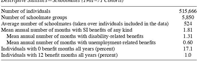
We now turn our attention to networks consisting of persons who went to the same ju-nior high school at the same point in time. Juju-nior high school in Norway is a three- year track, normally attended at ages 13–15. The total group of schoolmates during this period thus consists of fi ve birth cohorts: those at the same age, and those born up to two years before and two years after. We start out this subsection examining the peer effects present within this complete group. We then take a closer look at the importance of relational closeness, in this case measured by differences in class levels (age) and gender. Due to data limitations, we can only use a subset of our analysis population in this part of the analysis, namely those born between 1961 and 1971 (11 cohorts). To ensure that different birth cohorts really went to different classes, we also require the group of “levelmates” to comprise at least 30 persons. Finally, we remove siblings from each person’s peer group. In total, we construct data for 5,850 school-mate groups. Descriptive statistics are provided in Table 5.
Note that common shocks related to the schooling experience—such as being subject to a particularly good (or bad) principal or teacher—will not represent a confounder in this analysis because such events took place several years before our outcome period and, hence, presumably would be captured by the individual- fi xed ef-fects. It still may be the case, though, that persons who went to the same class / school are affected by the same shocks later on, as many of them continue to reside in the geographical area they grew up in. We control for this potential confounding factor in the same way as in the preceding subsection—that is, by including separate year dummy variables for each travel- to- work area (TWA) based on the address recorded at the start of the outcome period. In robustness analyses, we introduce year- dummies at lower geographical levels, all the way down to the neighborhood.
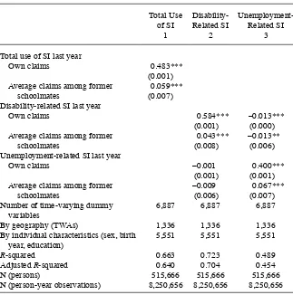
The results indicate signifi cant peer effects among former schoolmates; see Table 6. Looking fi rst at the total use of SI in Column 1, the peer effect is estimated to 0.059, which together with the autoregressive parameter implies a cumulative effect of 25 percent. Moving on to the separate models for disability- related (Column 2) and unemployment- related claims (Column 3), we again fi nd a pattern of positive direct effects and negative cross effects.
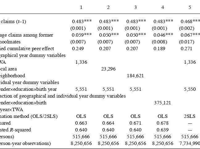
Robustness is evaluated in Table 7, where we control for potential time- varying local confounders at lower geographical levels. The estimated peer effects decline
slightly when we use separate year dummies at local area or the neighborhood levels. It is notable, though, that the estimated effects are unchanged when we substitute more than 185,000 neighborhood- year- fi xed effects for 23,000 locale- area- year- fi xed effects. The estimates again rise a bit when we use the fi rst- differenced 2SLS estimator rather than the fi xed effects OLS.
Most adults probably have little (if any) contact with the majority of the persons with whom they went to junior high school. Hence, by including all former school-mates in our peer measure, we clearly include a large number of irrelevant persons.
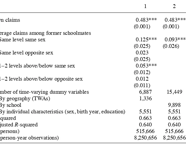
It therefore may be of some interest to distinguish “close” from more “distant” peers. In particular, we would guess that former classmates are more likely to maintain a relationship with each other than persons who went to different classes or levels. And it is also probable that same- sex persons have maintained more contact than persons of opposite sex. We examine the issue of relational closeness by estimating separate peer effects based on a same- level- same- sex distinction; see Table 8. Note that we have weighted each group’s SI average with its size relative to the total number of schoolmates (all fi ve cohorts), such that the coeffi cients are directly com-parable to each other and to the total schoolmate effect reported in Table 7. Again, the results indicate that relational closeness is a key factor in understanding social interaction effects. As shown in Column 1, the impact of same- level- same- sex peers is much larger than the impact of other schoolmates. And for schoolmates of the opposite sex, we fi nd no signifi cant peer effects at all. As an additional robustness exercise, we can take advantage of the differentiation between close and distant peers to check for possible confounding school- specifi c developments. In Column 2, we report the estimated same- level- same- sex peer effect in a model where we also include separate year dummy variables for each school included in the dataset. While these dummies may absorb some genuine peer effects related to the overall mass of schoolmates, we note that the estimated effect of the presumed closest peers declines only slightly.
C. Ethnic Minorities
Some of the most infl uential existing studies on social insurance interaction effects are based on data for ethnic minorities (Bertrand, Luttmer, and Mullainathan 2000; Aizer and Currie 2004; Åslund and Fredriksson 2009). We follow up on this literature
Table 5
Descriptive Statistics—Schoolmates (1961–71 Cohorts)
Number of individuals 515,666
Number of schoolmate groups 5,850
Average number of schoolmates (taken over individuals included in the data) 524
Mean annual number of months with SI benefi ts of any kind 1.81
Mean annual number of months with disability- related benefi ts 1.31
Mean annual number of months with unemployment- related benefi ts 0.60
Individuals with 0 benefi t months all years (percent) 17.1
by looking at SI use among immigrants from low- income countries.13 Our focus is on
immigrants who reside in areas where there are suffi cient numbers of other immigrants from the same country for a network of some size to be established. More specifi cally, we defi ne an ethnic minority network as a group of immigrants from the same origin country who resided in the same local area in 1992 (the “neighborhoods” discussed above are too small for this purpose). To be included in the analysis, we require a network size of minimum ten persons. Based on this strategy, we end up with 23,306
13. We disregard immigrants from high- income countries here, both because they do not tend to be concen-trated in particular geographical areas and because they do not tend to reside permanently in Norway.
Table 6
Main Estimation Results—Schoolmates (Standard Errors in Parentheses)
Total Use Average claims among former
schoolmates
Average claims among former schoolmates
Average claims among former schoolmates
Adjusted R- squared 0.640 0.704 0.454
N (persons) 515,666 515,666 515,666
N (person- year observations) 8,250,656 8,250,656 8,250,656
persons, divided between 746 local immigrant networks; see Table 9 for descriptive statistics.
One could imagine that the social interaction effects decrease with geographical distance for immigrants as well as for natives, suggesting that we should examine how the estimated effects change as we substitute close groups with more distant ones (but with the same nationality). Our data impose some limitations, however, as national-ity networks of the required size are typically located close together. Instead, we use immigrants from other low- income countries as candidates for more “distant” peers. In addition, we look at how immigrants are affected by SI use among natives within the same local area. Again, we compose the groups of other immigrants and natives such that they are of equal size and have similar characteristics as the person’s own same- nationality network. We are not able to obtain exact matches of the same quality as those used in the neighborhood analysis above, and the relatively low number of observations available for this analysis also implies that we cannot “afford” to drop observations with imperfect matches. Hence, while we have a perfect matching on sex, we allow for poorer matches on age and educational attainment. We are also not able to control for time- varying confounders at a lower level than travel- to- work areas. Note, however, that immigrants from different low- income countries typically work
Table 7
Robustness. Schoolmate Peer Effect on Total SI Use (Standard Errors in Parentheses)
1 2 3 4 5
Own claims (t–1) 0.483*** 0.483*** 0.483*** 0.483*** 0.468***
(0.001) (0.001) (0.001) (0.001) (0.002) Average claims among former
schoolmates
0.059*** 0.050*** 0.050*** 0.046*** 0.067*** (0.007) (0.007) (0.007) (0.008) (0.017)
Implied cumulative peer effect 0.249 0.207 0.207 0.189 0.271
Geographical year dummy variables
TWA 1,336 1,336
Local area 23,296
Neighborhood 184,621
Individual year dummy variables
Gender×education×birth year 5,551 5,551 5,551 5,550
Interaction of geographical and individual year dummy variables Gender×education×birth
year×TWA
375,121
Estimation method (OLS / 2SLS) OLS OLS OLS OLS 2SLS
R- squared 0.663 0.664 0.671 0.678 —
Adjusted R- squared 0.640 0.640 0.640 0.639 —
N (persons) 515,666 515,666 515,666 515,666 515,666
N (person- year observations) 8,250,656 8,250,656 8,250,656 8,250,656 7,734,990
Table 8
Total Use of SI. Estimated Peer Effects by Relational Closeness. Schoolmates (Standard Errors in Parentheses)
1 2
Own claims 0.483*** 0.483***
(0.001) (0.001)
Average claims among former schoolmates
Same level same sex 0.125*** 0.093***
(0.025) (0.026)
Same level opposite sex 0.023
(0.025)
1–2 levels above / below same sex 0.053***
(0.012)
1–2 levels above / below opposite sex 0.012
(0.011)
Number of time- varying dummy variables 6,887 15,449
By geography (TWAs) 1,336
By school 9,898
By individual characteristics (sex, birth year, education) 5,551 5,551
R- squared 0.663 0.663
Adjusted R- squared 0.640 0.640
N (persons) 515,666 515,666
N (person- year observations) 8,250,656 8,250,656
Notes: Individual fi xed effects are included. R- squared is a goodness- of- fi t measure for the complete model including the individual- fi xed effects. Standard errors are clustered at the peer group level. *(**)(***) indi-cates signifi cance at the 10(5)(1) percent level.
Table 9
Descriptive Statistics—Ethnic Minorities (1942–74 Cohorts)
Number of individuals 23,306
Number of immigrant networks 746
Average size of immigrant network (taken over individuals included in the data) 101.3
Mean annual number of months with SI benefi ts of any kind 3.87
Mean annual number of months with disability- related benefi ts 2.52
Mean annual number of months with unemployment- related benefi ts 1.53
Individuals with 0 benefi t months all years (percent) 9.3
in similar sectors of the economy, with a domination of low- skill service sector jobs (Bratsberg, Raaum, and Røed 2010); hence, if uncontrolled- for confounding factors remain at the local level, they would presumably affect persons from different low- income countries in a similar fashion.
Table 10 presents the results, including the 2SLS results for the main model. Ac-cording to the OLS estimates, there is a signifi cant peer effect among immigrants from a common source country—stronger than what we have found to be the case for neighbors in general and former schoolmates. The cumulative total SI peer ef-fect is around 38 percent. On the other hand, we fi nd no peer effects among immi-grants from different source countries and indications of a small negative effect of natives’ SI claims. The 2SLS point estimates are almost identical to OLS for these networks yet with much larger standard errors. Turning to the separate estimations for disability- related and unemployment- related claims, we again fi nd patterns of large positive direct effects and negative cross- effects.
D. Mechanisms
Peer effects can be driven by information sharing and by propagation of norms / stigma. While we would expect information sharing to be relevant for entry decisions only (or at least primarily), more general norm- effects are relevant for both entry and con-tinuation decisions. Hence, by examining peers’ infl uence on entry and continuation separately, we may gain some understanding of the underlying mechanisms. To do this, we have dichotomized the outcome variable used in the previous three subsec-tions (=1 for positive SI claims during a year, =0 otherwise), and split our data set into three (partly overlapping) parts. To examine infl ow into disability- related and unemployment- related SI, we use annual observations for which there were no SI claims last year (yi,t–1 = 0). To examine continuation of disability- related SI claims, we use observations for which there were some disability- related SI claims last year. And to examine continuation of unemployment- related SI claims, we use observa-tions for which there were some unemployment- related claims last year (persons with both disability- and unemployment- related claims last year are included in both the two latter groups). We then redo the main statistical analyses by program type—for neighbors, schoolmates, and ethnic minorities. Except that the lagged dependent vari-able drops out of the analyses, the statistical models, the peer varivari-ables, and the control variables are exactly the same as in previous subsections (see Tables 2, 6, and 10, respectively)—that is, OLS (in this case linear probability models) with person- fi xed effects and individual time- controls (based on TWA and combinations of gender, age, and education).
Table 10
Main Estimation Results—Nationalities (Standard Errors in Parentheses)
Total Use of SI Disability-
Immigrants from same source country 0.070*** 0.081*** (0.009) (0.021) Immigrants from other low- income country
(matched)
Immigrants from same source country 0.051*** –0.027***
(0.009) (0.010) Immigrants from other low- income country
(matched)
Immigrants from same source country –0.023*** 0.117***
(0.007) (0.010) Immigrants from other low- income country
(matched)
–0.008 –0.013
(0.007) (0.008)
Natives (matched) –0.002 –0.026*
(0.013) (0.015)
Estimation method (OLS / 2SLS) OLS 2SLS OLS OLS
Number of time- varying dummy variables 18,122 18,121 18,122 18,122
By geography (TWAs) 931 931 931 931
By individual characteristics (sex, birth year, education)
17,191 17,190 17,191 17,191
R- squared 0.719 0.603 0.603
Adjusted R- squared 0.684 0.554 0.554
N (persons) 23,306 23,306 23,306 23,306
N (person- year observations) 372,896 349,590 372,896 372,896