Ches Bay BC Assessment document final approved

(1)

STOCK ASSESSMENT OF

THE BLUE CRAB

IN CHESAPEAKE BAY

(2)

Ref [UMCES]CBL 11-011

Stock

Assessment

of

Blue

Crab

in

Chesapeake

Bay

2011

Final

Assessment

Report

Thomas J. Miller, Michael J. Wilberg

Amanda R. Colton

University of Maryland Center for Environmental Science

Chesapeake Biological Laboratory,

P. O. Box 38,

Solomons, MD

Glenn R. Davis, Alexei Sharov,

Fisheries Administration,

Maryland Department of Natural Resources,

Tawes Administration Building,

Annapolis, MD

Romuald. N. Lipcius, Gina M. Ralph

Virginia Institute of Marine Science, Gloucester Point, VA

Eric G. Johnson

Anthony G. Kaufman

Smithsonian Environmental Research Center

647 Contees Wharf Road

Edgewater, MD

Submitted to: Mr. Derek Orner

National Oceanic and Atmospheric Administration

Chesapeake Bay Office

Annapolis, MD

Submitted on 1 March 2011

Technical Report Series No. TS‐614‐11 of the University of Maryland Center for

Environmental Science.

(3)

Executive

Summary

The blue crab (Callinectes sapidus) is an icon for the Chesapeake Bay region. The commercial fisheries for blue crab in the Bay remain one of the most valuable fishery sectors in the Bay. Ecologically, blue crab is an important component of the Chesapeake Bay ecosystem. Thus, sound management to ensure the sustainability of this resource is critical.

The first bay wide assessment for blue crab was completed by Rugolo et al. in 1997. It concluded that the stock was moderately to fully exploited and at average levels of abundance. Subsequent to this assessment concerns over the continuing status of blue crab were raised because of declines in abundance and harvests. In response to concerns from stakeholders, a Bi‐State Blue Crab Advisory Committee was established in 1996. Work by this committee led to the establishment in 2001 of biomass and

exploitation thresholds and an exploitation target reference point. The stock was assessed again in 2005 by Miller et al. This assessment analyzed fishery‐dependent and fishery‐independent data to assess the status of the blue crab population in the

Chesapeake Bay. Population status was compared to reference points developed from an individual‐based yield per recruit analysis which used the exploitation rates

equivalent to maintaining 10% and 20% of the virgin spawning potential. The

assessment recommended adoption of an exploitation fraction based management

regime with an overfishing definition equivalent to F10% = Uthreshold= 53% of all available crabs and a target exploitation rate of F20% = Utarget = 46%. Based on these reference points, the assessment concluded that exploitation rates in the fishery were too high. Since 2005, the status of the blue crab stock has been updated annually and its status determined relative to these reference points.

In 2009, we proposed and were funded to complete a thorough revision of the stock assessment for the blue crab in Chesapeake Bay. The following terms of reference were adopted to guide our assessment activities. We sought to (i) critically assess and where necessary revise the life history and vital rates of blue crab in the Chesapeake Bay that are relevant to an assessment of the stock, (ii) evaluate and recommend biological reference points for the Chesapeake Bay blue crab population. The potential for implementing sex‐specific reference points should be evaluated. (iii) describe and quantify patterns in fishery‐independent surveys. Analyses should include an evaluation of the impacts of environmental and abiotic factors on survey catches, to maximize the information content of resultant survey time series. (iv) describe and quantify patterns in catch, effort and survey‐based estimates of exploitation by sector and region, including analyses that examine the impacts of reporting changes and trends in CPUE, (v) develop and implement assessment models for the Chesapeake blue crab fisheries. In particular, models that permit estimates of the trends and status of the crab

(4)

approaches, (vii) characterize scientific uncertainty with respect to assessment inputs and stock status and (viii) evaluate stock status with respect to reference points.

We developed and implemented a sex‐specific catch, multiple survey model to develop integrated estimates of management reference points and stock status. This model represented the blue crab population in Chesapeake Bay of being composed of abundances. The best fitting model indicated a coefficient of proportionality between the abundance of age‐0 crabs in the winter dredge survey and total abundance of q0=0.4. This estimate leads to considerable changes in the interpretation of reference points and trajectory of the stock.

In implementing the model, we developed female‐specific exploitation rate and female‐specific abundance reference points. We recommend that all exploitation‐based reference points should be based on an estimate of the exploitation fraction of age‐0+

Atlantic Fishery Management Council, we recommend a target exploitation

rate be established equivalent to 0.75* UMSY. Our best estimate of the target exploitation rate is U0.75*UMSY=0.255 age ‐0+ female crabs.

3) We recommend an overfished abundance threshold be established based on

(5)

million age‐1+ female crabs. This is equivalent to a total population abundance of approximately 135 million age‐1+ crabs if the pattern of exploitation is the same for males and females.

4) We recommend that a target abundance reference point be established

equivalent to the equilibrium abundance expected if the target exploitation rate is achieved. Specifically, the target abundance should be defined as N0.75*UMSY. Our best estimate of the target abundance is 215 million age‐1+ female crabs. This is a level of abundance that was observed in the population in the mid‐1980s. The recommended target is equivalent to a total population abundance of approximately 415 million age‐1+ crabs if the pattern of exploitation is the same for males and females.

We recommend that the management control rules defined above are implemented

using empirical data from the winter dredge survey. Based on this approach, in 2009 the blue crab stock in the Chesapeake Bay was not overfished, nor was it experiencing overfishing. More specifically, the exploitation rate in 2009 (U2009 =0.24 age‐0+ female crabs) was below the Utarget = 0.255. Also, the blue crab population in 2009 was above the overfished definition of 70 million age‐1+ females. The best estimate of the

abundance in 2009 (N2009 = 174.3 million age‐1+ female crabs) was lower than the target abundance. We note that the abundance of crabs in the winter dredge survey of 2009‐ 2010 suggest that the population was above target abundance in 2010. Inspection of the stock trajectory indicated that the stock had experienced overfishing from 1998‐ 2004 and was technically overfished from 2001‐2003.

Effective conservation of the blue crab requires an understanding of the

relationships between exploitation rate, catch, and population abundance. Our analyses of temporal patterns in abundance and exploitation indicated that they were

approximately mirror images of each other, suggesting depensatory exploitation.

Consequently, precautionary management measures will be required when the blue

crab population is at low abundance to prevent population collapse.

Our analyses indicate that the stock responded favorably to management

measures aimed at conserving female crabs. Management measures likely led to an increase in the abundance of age‐1+ female crabs such that the recommended

(6)

Table

of

List

of

Tables

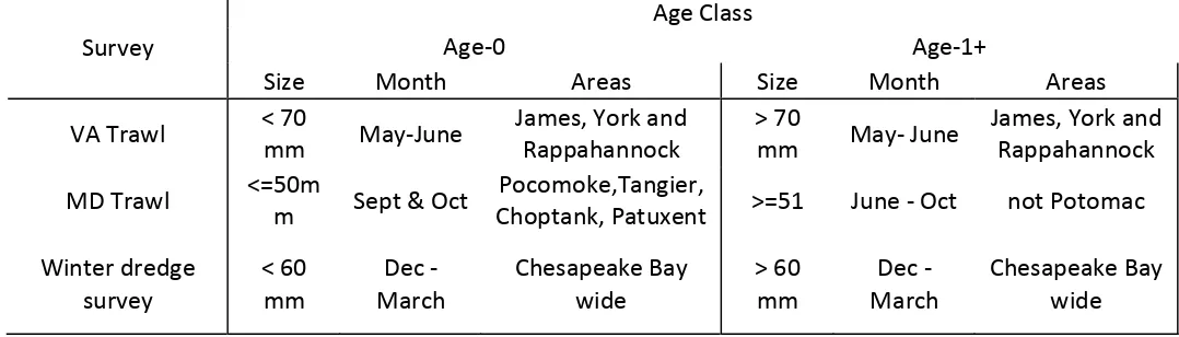
Table 3.1. Summary of size, times and areas used in calculating fishery‐independent crab abundance indices for the Chesapeake Bay ... 69 Table 3.2. Time series of area‐weighted geometric means for blue crab from the spring

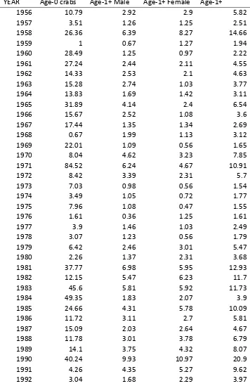
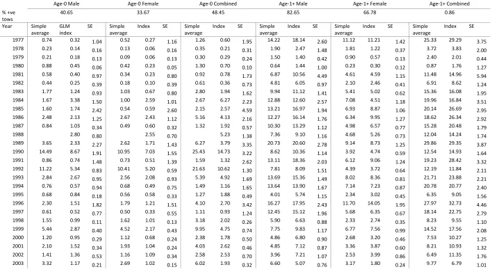
VIMS trawl survey for 1956‐2009. ... 70 Table 3.3. Results of generalized linear modeling of the data from the Maryland DNR

blue crab trawl survey (1977‐2009) ... 72 Table 3.4. Summary of model selection results for the Maryland DNR blue crab trawl

survey for A) Age‐0 male crabs, B) Age‐0 female crab and C) Age‐0 combined crabs. ... 74 Table 3.5. Summary of model selection results for the Maryland DNR blue crab trawl

survey for A) Age‐1+ male crabs, B) Age‐1+ female crab and C) Age‐1+ combined crabs. Shown are models for probability of occurrence and abundance given

occurrence ... 76 Table 3.6. Annual summary by sex and age of crabs collected in the winter dredge

survey. Estimates provided in the table are absolute abundances ... 78 Table 3.7. Summary of model selection results for the Winter Dredge Survey for A)

Age‐0 male crabs, B) Age‐0 female crab and C) Age‐0 combined crabs. ... 79

Table 3.8. Summary of model selection results for Winter Dredge survey for A) Age‐1+ male crabs, B) Age‐1+ female crab and C) Age‐1+ combined crabs. Shown are models for probability of occurrence and abundance given occurrence. ... 81

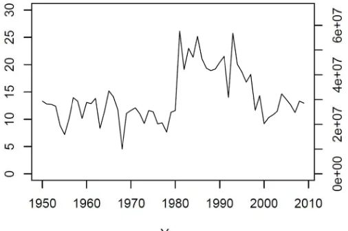
Table 5.1. Reported commercial landings for Virginia, Maryland and the Potomac River. ... 83

Table 5.2. Results of intervention analysis for the Virginia commercial landings for the period 1950‐2009 ... 86

Table 5.3. Results of intervention analysis for the Maryland commercial landings for the period 1950‐2009. ... 87

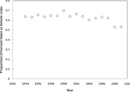
Table 5.4. The average sex ratio in the catch based on data from sex‐specific landings 1994‐2006 ... 88

Table 5.5 Reported sex‐specific landings for the three Chesapeake Bay jurisdictions. .. 89

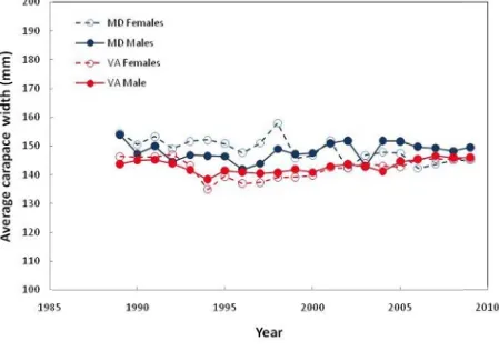
Table 5.6. The average size (carapace width) and resultant average weights (based on Eq. 3) in each of the three jurisdictions for the period 1989‐2009 ... 90

Table 5.7 Estimated landings in the Chesapeake Bay by number (Millions) for the years 1985‐2009. ... 91

Table 6.1 . Variable and parameter definitions for SSCMA model ... 92

(9)

List of Figures

Figure 1.1. Conceptual management control rule used in managing blue crab fisheries in Chesapeake Bay. ... 96

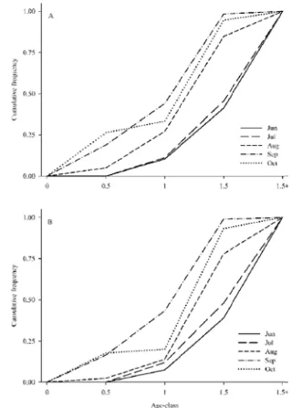
Figure 2.1. Cumulative partial recruitment of field‐collected blue crabs grouped into lipofuscin‐based age‐classes in (A) the peeler–soft crab fishery and (B) the hard crab fishery by month from June to October (from Puckett et al. 2008). ... 97 Fig. 2.2. Summary of direct empirical (symbols) and indirect (histogram) estimates of

natural mortality rate (M) of blue crab (Hewitt et al. 2007). ... 98 Figure 2.3. Annaul survival estimates (S) of mature female blue crab from a tag‐

recapture program conducted in the Chesapeake Bay from 2001‐2010. ... 99 Figure 3.1 Size frequency plots from the winter dredge survey for 1990‐2010. The

vertical line on each figure represents the 60 mm carapace width size bin. ... 100 Figure 3.2. Example distribution of stations in the three principal fishery‐independent

surveys. ... 101 Figure 3.3. Time series of age‐0 crab abundance in the VIMS spring trawl survey (1956‐

2009). ... 102 Figure 3.4. Age‐1+ crab indices for the VIMS spring trawl. ... 103 Figure 3.5. The relationship between survey indices of age‐1 crab abundance for

females, males and both sexes combined for the VIMS spring trawl survey ... 104 Figure 3.6. Correlation of lagged indices for the VIMS spring trawl survey ... 105 Figure 3.7 Frequency distribution of observed values of environmental parameters

measured during the Maryland DNR blue crab trawl survey (1977‐2009). ... 106 Figure 3.8. The distribution of catches of age‐0 crabs in the Maryland blue crab trawl

survey (1977‐2009) for A) Male crabs, B) Female crabs and C) Both sexes combined. ... 107

Figure 3.9. The distribution of catches of age‐0 crabs in the Maryland blue crab trawl survey (1977‐2009) for A) Male crabs, B) Female crabs and C) Both sexes combined. ... 108

Figure 3.10. Age‐0 crab standardized indices for the Maryland blue crab trawl survey. Shown are plots for age‐0 male, age‐0 female and age‐0 combined. ... 109

Figure 3.11. The relationship between GLM indices of age‐0 crab abundance for females, males and both sexes combined for the Maryland blue crab trawl survey. ... 110

Figure 3.12. Age‐1+ crab standardized indices for the Maryland blue crab trawl survey. ... 111

Figure 3.13. The relationship between GLM indices of age‐1+ crab abundance for females, males and both sexes combined for the Maryland blue crab trawl survey. ... 112

Figure 3.14. Correlation of lagged indices for the Maryland blue crab trawl survey. ... 113

(10)

Figure 3.17 Summarized catch distributions in the winter dredge survey by age and sex.

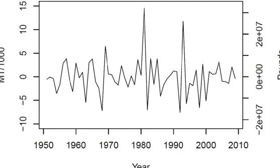
Figure 5.3. Reconstructed Virginia commercial landings. Landings were reconstructed based on the estimated impact of the 1993 reporting change to mandatory

reporting. ... 126

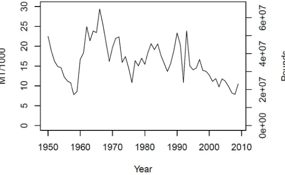
Figure 5.4. Annual reported commercial landings in Maryland for the period 1950‐2009. ... 127

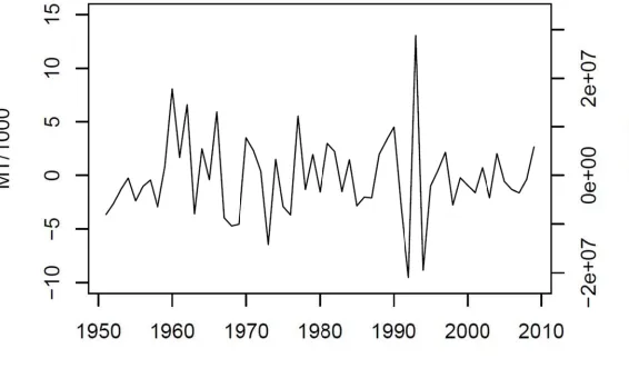
Figure 5.5. First differenced time series of reported commercial landings in Maryland for the period 1950‐2009. ... 128

Figure 5.5. Reconstructed Maryland commercial landings. ... 129

(11)

Figure 6.4. Time series of predicted and estimate catch (upper panel), female catch (middle panel) and male catch (bottom panel ) resulting from the base run of the SSCMSA. ... 139 Figure 6.5. Time series of predicted and estimates of survey CPUES in the VIMS spring

trawl survey for recruitment (upper panel), age‐0+ females (middle panel) and age‐ 1+ males (bottom panel ) resulting from the base run of the SSCMSA. ... 140 Figure 6.6. Time series of predicted and estimates of survey CPUES in the Maryland DNR Summer trawl survey for recruitment (upper panel), age‐0+ females (middle panel) and age‐1+ males (bottom panel ) resulting from the base run of the SSCMSA. .. 141 Figure 6.7. Time series of predicted and estimates of survey CPUES in the winter dredge

survey for recruitment (upper panel), age‐0+ females (middle panel) and age‐1+ males (bottom panel ) resulting from the base run of the SSCMSA. ... 142 Figure 6.8 Comparison of observed and model predicted values of recruitment for the

VIMS trawl survey (upper panel), MD DNR trawl survey (middle panel) and the winter dredge survey (lower panel). ... 143 Figure 6.9. Trends in female age‐1+ abundance (upper panel) and male age‐1+

abundance predicted by the base run of the SSCMSA model. Solid lines indicate

maximum likelihood estimates, and dashed lines indicate approximate 95%

confidence intervals ... 144

Figure 6.10. The female exploitation rate, male exploitation rate, and the ratio of male‐ specific exploitation to female specific exploitation estimated from the base run of the SSCMSA. Solid lines indicate maximum likelihood estimates, and dashed lines indicate approximate 95% confidence intervals. ... 145

Figure 6.11. Predicted yield curves for the base model as a function of the exploitation rate on age‐1+ female crabs. ... 146

Figure 6.12. Predicted yield curves for the base model as a function of the exploitation rate on age‐0+ female crabs. ... 147

Figure 6.13. Predicted yield curves for the base model as a function of the abundance of age‐0+ female crabs. ... 148

Figure 6. 14. Relationship between the sex‐specific ratio of exploitation rates

(Fmale:Ffemale )and the equilibrium number of female crabs in the population at MSY. ... 149

Figure 6.15. Recommended revised control rule for the blue crab fishery in Chesapeake Bay based on revised reference points developed in the SSCMSA and the empirical estimate of stock history estimated from the reported female catch and the

estimated female abundance from the winter dredge survey... 150

Figure 6.16. A control rule developed from the application of the updated CMSA model (Miller et al. 2005). All parameters in the model fit were as specified in the 2005 assessment. ... 151 Figure 6.17. A control rule developed from the application of the standardized CMSA

(12)

1

Terms

of

Reference

The 2011 stock assessment of blue crab in the Chesapeake Bay was funded by grants from the NOAA Chesapeake Bay Office, the Maryland Department of Natural

Resources and the Virginia Marine Resources Commission. There were two components

to the project: a benchmark stock assessment and research activities in support of the assessment and management. This report focuses on the assessment activities: the research results will be reported elsewhere.

The stock assessment has the following eight specific terms of reference.

TOR 1: Critically assess and where necessary revise the life history and vital rates of blue crab in the Chesapeake Bay that are relevant to an assessment of the stock. TOR 2: Evaluate and recommend biological reference points for the Chesapeake Bay blue crab population. The potential for implementing sex‐specific reference points should be evaluated.

TOR 3: Describe and quantify patterns in fishery‐independent surveys. Analyses should include an evaluation of the impacts of environmental and abiotic factors on survey catches, to maximize the information content of resultant survey time series.

TOR 4: Describe and quantify patterns in catch, effort and survey‐based estimates of exploitation by sector and region, including analyses that examine the impacts of reporting changes and trends in CPUE.

TOR 5: Develop and implement assessment models for the Chesapeake blue crab fisheries. In particular, models that permit estimates of the trends and status of the crab population and fisheries on a sex‐specific basis should be

evaluated.

TOR 6: Examine density‐dependent exploitation patterns derived from survey‐based

and model‐based approaches.

TOR 7: Characterize scientific uncertainty with respect to assessment inputs and stock status.

TOR 8: Evaluate stock status with respect to reference points.

1. Introduction

(13)

background information sufficient to evaluate the assessment. The blue crab

(Callinectes sapidus) is one of fourteen swimming crab species in the genus Callinectes

(Williams 2007). Nine of the fourteen swimming crabs, including the blue crab are endemic to the western Atlantic basin, mainly in tropical and subtropical areas. The distribution of the blue crab is much wider than those of conspecific species as it ranges from Uruguay to Massachusetts, with occasional records from Argentina to Nova Scotia (Williams 1974, Norse 1977). In addition to its endemic range, the species has become established as an exotic in the Mediterranean basin (Holthuis 1961, Banoub 1963).

Throughout its range, the blue crab is an important component of estuarine ecosystems (Hines 2007). Blue crabs are dominant and opportunistic benthic predators and scavengers (Eggleston et al. 1992, Hines 2007). Their diets may include a wide range of taxa including bivalves, crustaceans and fish (Hines et al. 1990, Mansour and Lipcius 1991). It is a dominant benthic predator and scavenger (Eggleston et al. 1992). Diets vary with crab size. Small crabs exploit thin‐shelled bivalves and other

invertebrates that are buried relatively shallowly in the sediments. Larger crabs can exploit thicker‐shelled bivalves and cannibalism is not uncommon (Dittel et al. 1995, Hines and Ruiz 1995). Thus, crabs may be keystone predators in the estuary, sensu

Paine (1966), possibly playing a dominant role in structuring benthic communities throughout its range.

In addition to its ecological importance, the blue crab supports important

commercial and recreational fisheries throughout much of its range. Blue crab has been harvested since pre‐colonial times. The commercial fishery started in earnest in the mid‐nineteenth century (Cronin 1998, Kennedy et al. 2007). Commercial landings are regularly reported from coastal states from Texas to Connecticut1. In the last decade larger and more consistent landings have been reported from the more northerly states of New York, Connecticut and Rhode Island (K. McKowen, NY Department of

Environmental Conservation, pers. comm.). In the 1950’s, the Chesapeake Bay region represented almost 80% of the national landings. This figure has fallen steadily since then, so that based on the last 10 years (2000‐2009), the Chesapeake Bay represents only 34% of the national landings. However, there is some evidence of an increase in importance of the Chesapeake region in the last two years (Average2008‐2009 = 42.2% )

Maryland, Virginia and the Potomac River Fisheries Commission are the

management jurisdictions for blue crab in Chesapeake Bay. The management actions of the three jurisdictions are coordinated since all are signatories to the Chesapeake Bay

1

(14)

3

Blue Crab Fishery Management Plan (FMP ‐‐ Chesapeake Bay Program 1997). The FMP

provides recommendations for the management of commercial and recreational fishing

of blue crab in the Bay. Its goal is “to manage blue crabs in the Chesapeake Bay to conserve the bay wide stock, protect its ecological value, and optimize the long‐term utilization of the resource.” The blue crab FMP adheres to the principles proposed for Chesapeake Bay FMPs that were developed by the Chesapeake Bay Program in 1998, in which precautionary management and protection of critical habitats are highlighted.

Regulations and management actions are complementary across the jurisdictions, but

recognize age‐specific and sex‐specific differences in utilization of the estuary by blue crab, and historical fishing patterns.

More recently, blue crab has been selected as one of five key species at the heart of the Maryland Sea Grant Ecosystem‐based Fisheries Management project. As a part of this initiative, a comprehensive briefing document was synthesized from

available scientific information to identify the major biological, ecological and economic stressors acting on the blue crab and the fisheries it supports (EBFM Blue Crab Species Team 2010). The EBFM blue crab brief identified several indicators of population health including patterns of connectivity at local and regional scales, recruitment variability and

mortality processes.

1.1. Assessment

History

Studies of the dynamics of blue crab in the Chesapeake Bay began as early as the late 19th Century. Considerable efforts were made in subsequent years to understand the dynamics of the blue crab population in Chesapeake Bay. These initial studies documented growth, spawning periodicity and population variability (Hurt et al. 1979). However, it was not until 1997 that the first baywide assessment of blue crab in the Chesapeake was completed (Rugolo et al. 1997). This first comprehensive assessment was conducted under the auspices of the Chesapeake Bay Stock Assessment Committee (CBSAC). Rugolo et al. (1997) used index‐based approaches and a simple production model in their assessment. They indicated that stock abundance had been high in the 1980s and had declined to more average abundances over the subsequent decade. The authors noted a decrease in catch‐per‐unit‐effort (CPUE) in the blue crab fishery since 1945. But no consistent decreases were evident in survey‐based CPUE or fishing mortality rates. Rugolo et al. attributed these counter‐intuitive results to gear

(15)

the exploitation levels then occurring. Rugolo et al. recommended establishing and maintaining a fishing mortality rate reference point that ensured escapement of at least 10% of the virgin spawning potential. Although finding no cause for alarm, Rugolo et al. recommended no further increases in fishing effort or fishing mortality.

Following the Rugolo et al. (1997) assessment, Miller and Houde (1999) revisited the assessment of the blue crab fishery to develop threshold and target reference points. The Miller and Houde report is available online at

http://hjort.cbl.umces.edu/crabs/doc/Final_targeting_report.pdf. Miller and Houde recommended a hierarchy of target levels, designated to address sustainability,

efficiency, and recovery scenarios. Targets were derived from 1) reported catches and effort in the commercial fishery, 2) statistics from fishery‐independent surveys, and 3) knowledge of the biology of blue crab. Targets recommended included population sizes, catches, and effort levels, as well as reference fishing mortality rates. They were

intended to be conservative and risk‐averse and promote a sustainable and

economically viable fishery, while protecting the ecological value of the blue crab in Chesapeake Bay. In the hierarchy, the first targeting level was one that designated population abundances and fishing mortality rates to ensure sustainability of the

resource. Miller and Houde recommended a long term potential yield of ~36,000 metric tonnes (MT ~ 80 million Lbs.) and fishing mortality rates of F < 0.9. A second target level

equivalent to F=0.6 was recommended to ensure that the maximum reproductive

potential per crab would be obtained over the long term. A recovery target was also recommended of F <0.5 to help build the stock in the case of recruitment overfishing. Some of the recommendations from the Miller and Houde assessment differed

substantially from the earlier assessment as these authors interpreted the effects of a reporting change that occurred in Maryland in 1981 differently than had Rugolo et al. (1997). Fogarty and Miller (2004) demonstrated the impacts of reporting changes in the blue crab fisheries and argued that accounting for them would be important in future

assessments.

In 1996, the Governors and Legislatures of Maryland and Virginia established the “Bi‐State Blue Crab Advisory Committee” (BBCAC) to provide them with independent advice on the status and future trends of the blue crab fisheries. In 1998, BBCAC endorsed the findings of its technical work group that indicated that there were signs that the crab population was not in a healthy condition. Specifically BBCAC identified the following indicators of concern:

 Overall abundance for all age groups was down,

 Fishing mortality was increasing,

(16)

5

 Spawning stock biomass was below the long‐term average,

 The average size of crabs was decreasing,

 Fishery‐independent surveys showed a decreasing percentage of legal size crabs,

 The reproductive potential of the population was of concern because of the reduced size of males and lack of mature females.

This consensus view motivated the development of a new management

framework for the Chesapeake Bay blue crab fisheries (Miller 2001b). The framework recognized the need to distinguish between threshold and target reference points. The

document is available online at http://hjort.cbl.umces.edu/crabs/docs/Charette_01.pdf.

Specifically, the framework identified biomass‐ and exploitation‐based threshold reference points that bounded a zone of sustainable exploitation (Fig. 1.1). Within this zone of sustainable exploitation, researchers recommended a target exploitation rate that sought to double the current spawning potential of the blue crab population (Fig. 1.1). In making these control rules functional, empirical evidence and elementary per recruit analyses were combined to determine values for the threshold and target reference points. The abundance threshold reference point was determined to be the lowest standardized abundance (Z‐score) that had been observed in the average of three fishery‐independent surveys. This was determined to be the value observed in 1968. The justification for this choice was that evidence was lacking to suggest that lower abundances could support a sustainable fishery. The fishing mortality rate threshold was determined from a standard spawning potential per recruit analysis. A value of F10% (F=1.0) was chosen based on previous precedence and because the value indicated was greater than the majority of fishing mortality rates that had been observed previously. The target reference point was chosen as F20% (F=0.7). This level was chosen as it was believed to be sufficiently far from the threshold reference points as to be detectably different, and because it would lead to an effective doubling of the spawning stock present in 2001.

Miller et al. (2005) produced the next full assessment of the blue crab stock and its fisheries in Chesapeake Bay. The full assessment is available online at

http://hjort.cbl.umces.edu/crabs/Assessment05.html. These authors reviewed key life history parameters for blue crab. In particular, they reviewed direct and indirect estimates of the rate of natural mortality, M (Hewitt et al. 2007). Importantly, Miller et al. recommended abandoning the M = 0.375 value used by Rugolo et al. (1997) in favor of a revised M=0.9 estimate. This increased level of M was used throughout the

(17)

The changes in M and in the methodological approach yielded new values for the target and threshold reference points, although the definitions of the reference points (i.e., 20% and 10% virgin spawning potential) were maintained. However, Miller et al. (2005) expressed these reference‐points not in terms of instantaneous rates (e.g., F) but in terms of the target and threshold exploitation fractions (U) equivalent to the 20% and 10% spawning potential ratios. Specifically, Miller et al. (2005) calculated values of Utarget=0.46 and Uthreshold=0.53. Miller et al. (2005) maintained the definition of the overfished threshold as the abundance equivalent to the lowest abundance observed in the baywide winter dredge survey (Miller et al. 2001c), but expressed this value in terms of absolute abundance rather than as a standardized value. To assess the status of the blue crab stock against these reference points, Miller et al. (2005) used a catch‐survey model (Collie and Sissenwine 1983), modified to include multiple fishery‐independent surveys. Based on this new framework, Miller et al. (2005) concluded that the blue crab stock in 2005 was not overfished nor was it experiencing overfishing.

The Miller et al. (2005) assessment was reviewed by an international panel of independent experts. The review team concluded that the 2005 assessment

represented the best science then available and therefore provided a sound basis for

management (http://hjort.cbl.umces.edu/crabs/Assessment05.html). Subsequent to

the acceptance of the assessment, the management jurisdictions implemented policies

aimed at reducing exploitations fractions to the target level of Utarget=0.46.

No major new integrated analyses have been conducted since the Miller et al.

(2005) assessment. However, several modifications to the management framework

have been made by CBSAC. Perhaps most significantly, stock status is now determined annually using a purely empirical approach. The abundance of crabs is estimated using the winter dredge survey (see Section 3.2.4) and the exploitation fraction is calculated as the harvest during the year divided by the observed winter dredge survey abundance at the beginning of the year. The catch survey model is not used in the annual

determination of stock status. In 2008 an interim abundance target was established, equal to 200 million crabs (Chesapeake Bay Stock Assessment Committee 2008). This figure was based on analyses of the relationship between winter dredge‐based estimates of abundance and harvest, and abundance and recruitment. Moreover, in 2008 CBSAC noted that management actions had yet to achieve the target exploitation

rate and recommended adoption of management policies that focused on conserving

(18)

2. Biology

and

Life

History

2.1. Stock

Structure

Population structure of blue crab within its range remains somewhat uncertain. In 1994, McMillen‐Jackson et al. (1994) used a protein electrophoretic approach to quantify the genetic variability in samples collected from Texas to New York. This research indicated moderate genetic structuring, with spatial patchiness of several loci evident throughout the range. However, the findings also indicated that a high level of regional gene flow acted to diminish population structure. Recently, these researchers have revisited the question of population structure within the blue crab using multiple genetic markers and restriction length fragment polymorphism analysis of mitochondrial DNA (McMillen‐Jackson and Bert 2004). The genetic results indicated no clear split between Gulf of Mexico stocks and Atlantic coast stocks. However, there was, within the Atlantic coast a cline of genetic diversity, with the New York samples exhibiting significantly lower diversity than more southerly stocks. The authors inferred from these patterns a latitudinal expansion from a sub‐tropical center of diversity.

Furthermore, the maintenance of a cline in diversity suggests that local gene flow may be low or restricted. Recently, Al Place and colleagues at the UMCES Institute of Marine

and Environmental Technology have sequenced the mitochondrial genome of blue crab.

These researchers documented genetic markers that distinguished among crabs in the Chesapeake Bay, but have yet to identify markers that can separate crabs among estuaries. Thus, definitive statements about the spatial scale of population structure are still lacking. Although there is no definitive evidence of genetic structuring

indicative of separate populations, there is clear evidence of localized populations that experience limited gene flow between them. In summary, the genetic evidence suggests the existence of, at a minimum, a functionally separate Chesapeake Bay blue crab stock that experiences only limited exchange of individuals with neighboring stocks.

(19)

zoea occur in distinct patches 0.5 – 2.5 km diameter in the vicinity of the mouth of Delaware Bay. Modeling studies by Garvine et al. (1997) indicated that some larvae return to Delaware Bay using upwelling‐favorable wind events. However, these

modeling studies also indicated that a not insignificant proportion of zoea are advected southward in a buoyancy driven coastal current. These larvae may represent potential recruits to the Chesapeake Bay population. Studies of recruitment in the Chesapeake Bay stock indicate a similar picture to that found for Delaware. Roman and Boicourt (1999), found patches of zoea associated with the Chesapeake Bay plume front. In a numerical analysis Johnson and Hess (1990) estimated that only 13% of released zoea remained in the Chesapeake Bay and that the remaining zoea (87%) are advected out to sea. Johnson and Hess (op. cit.) calculated that 29% of the zoeal production returns to the Chesapeake Bay. It is important to note that these figures do not include zoeal mortality, which is likely to be substantial, and thus represent an upper bound.

From this review, we conclude that there is sufficient evidence to support the assumption that the blue crab population in the Chesapeake Bay comprises a unit stock, at least for assessment purposes. This does not imply that there is no exchange with or subsidy from neighboring populations; rather it assumes that the dynamics of the Chesapeake Bay population are determined from internal considerations, and not from subsidies or exchanges with other populations. Subsidies and exchanges do likely occur with genetic and evolutionary implications– we are simply assuming that they are not significant to population dynamics. However, we note that such subsidies and

exchanges are likely to be more important when the size of the Chesapeake Bay population is small.

2.2. Growth

Information on blue crab growth dynamics has expanded substantially since the last assessment (Miller et al. 2005). Three factors underlie this increase in knowledge: liposfuscin‐based ageing (Ju et al. 2001), molt‐process modeling (Brylawski and Miller 2006) and stock enhancement efforts (Zohar et al. 2008).

The physiology and energetics of growth in blue crab were summarized by Smith and Chang (2007). However, documenting the growth dynamics of blue crab and other crustaceans in the field is difficult because of the lack of structures for ageing.

(20)

et al. 1999). Crabs raised in artificial ponds were held at ambient conditions, allowed to forage on naturally abundant prey and sampled on several occasions over 18 months. Information on the sizes of known age crabs from the ponds were fit to a von

Bertalanffy growth function. Puckett et al. (2008) used the lipofuscin assay to age free‐ living crabs in the Chesapeake Bay. These authors concluded that the peeler‐soft crab and the hard crab fisheries exploit crabs less than 18 months of age (Fig. 2.1).

Smith (1997) developed a discrete molt‐process model for blue crab in the Chesapeake Bay. He used empirical relationships developed for crustaceans generally to develop a specific parameterization for blue crab. Using this approach, Smith estimated von Bertalanffy parameters that best described the growth trajectory generated. These model parameters yielded estimates of sizes at the onset of

overwintering in the first, second and third years of 32.5, 107.5 and 147.6 mm carapace width (CW). Brylawski and Miller (2006) conducted laboratory experiments to directly estimate the parameters of Smith’s molt process model. These authors incorporated their parameter estimates into a simulation model which demonstrated that observed variability in winter temperatures could vary the timing of recruitment to the fishery by up to 10%.

Recent research efforts to assess the feasibility of stock enhancement for blue crabs in Chesapeake Bay have generated new information on growth. Growth data are available from two components of this project (1) growth of early life stages during the development of aquaculture technologies and (2) growth of larger juveniles and adults from experimental field releases of hatchery‐reared animals. Zmora et al. (2005) cultured juvenile crabs in a hatchery from captive spawning adults; zoea grew to 1st stage juveniles (C1) in approximately one month, and from C1 to C6‐7 stage (~20 mm CW) in the subsequent month. Although, no quantitative estimates are given, Zmora et al. (2005) noted striking variability in growth rates among individuals in a single brood. Releases of hatchery‐reared blue crab juveniles into shallow water habitats of the upper and lower Bays provided the opportunity to estimate growth rates of free‐ranging animals under natural conditions (Davis et al. 2005, Hines et al. 2008). Similar to previous studies, growth was temperature‐dependent with peak growth rates of 1.2 mm CW d‐1 observed in July. A deterministic growth model based on field data predicts that juveniles recruiting in fall will enter the hard crab fishery during late summer to early fall of the following year. Growth rates of hatchery‐reared animals appear to be representative of wild crabs; paired experimental releases of hatchery‐reared and wild cohorts showed no difference in observed growth rates (Johnson et al. In press).

2.3. Reproduction

(21)

2.3.1. Molt to maturity

Blue crabs reproduce sexually, and males and females are sexually dimorphic

and exhibit different growth forms. The reproductive physiology and anatomy are reviewed by Jivoff et al. (2007). Circumstantial evidence strongly suggests the presence of a terminal molt in female blue crab (Van Engel 1958, Abbe 1974). Limited

physiological evidence suggests that the Y‐organ does not degenerate as it does in other crabs that exhibit determinate growth, rather Smith and Chang (2007) speculate that in blue crab it is over production of MIH by the X‐organ that enforces the terminal molt. As the Y‐organ does not degenerate, female crabs maintain the physiological capacity to molt again under rare circumstances. Evidence for a terminal molt in males is less definitive than in females. There is some evidence for continued growth in males, particularly as most of the largest crabs collected are males. However, similarly to large females, large males form limb buds when they lose an appendage, and such males are often collected in the field suggesting that males molt infrequently at large sizes.

2.3.2. Age and size at maturity

Our limited ability to age blue crabs has precluded empirical development of maturity ogives for blue crab. However, recent evidence from attempts to develop large scale aquaculture of blue crabs at the Institute for Marine and Environmental Technology, indicate that females can mature within their first year under ideal conditions. In the field, given the annual temperature cycle and typical megalopal settlement dates in August and September, it is unlikely that crabs could mature within their first year. It is more likely that they mature in the autumn of the following year when they are 12‐18 months of age. Those that do not mature at this time, likely delay maturity for a following year, and mature when they are 24‐30 months old. Hester et al. (1982) reviewed information on age at maturity in Chesapeake Bay. Their review

suggested two production schedules: those females originally hatched in May reach maturity in 15 months and spawn at 24 –27 months of age, and those crabs originally hatched in August reach maturity in 21 months and spawn at 24 months. More recently, Hines et al. (2003) suggest that although females in different parts of the bay may mature at the same time, they differ in the timing of larval release (see Section 2.4.3).

2.3.3. Mating and spawning periods and locations

(22)

Kendall and Wolcott 1999). Males that mate frequently transfer less sperm which impacts the number of zoea released subsequently by mated females (Hines et al. 2003). Mating typically occurs from May – October (Hines et al. 2003). Mating pairs have been reported widely throughout the Chesapeake Bay system. Hines et al. (2003) found that 98% and 100% of mature females in the Rhode River and lower Bay held ejaculate stores, indicating a high level of mating success in the field.

Following mating, the behavior of inseminated females can differ depending on their mating location (Hines et al. 2003, Aguilar et al. 2005). Females inseminated in the upper Bay in the summer and fall will migrate southward towards the lower Bay in late fall, overwinter and release larvae in the summer of the following year. Current

evidence suggests that none of the females inseminated in upper Bay sub‐estuaries will produce broods during the same year as mating. Similar to females mating in the upper bay, most females inseminated in the lower Bay probably follow this same timing of brood production. However, unlike upper Bay females it is likely that some unknown fraction of females inseminated in the lower Bay can release larvae in the same season in which they were inseminated. Prior to hatching, ovigerous females migrate to the high salinity waters at the mouth of the Chesapeake Bay (Tankersley et al. 1998).

Hatching occurs around nocturnal high tide and zoea are carried seaward on the ensuing ebb current.

2.3.4. Fecundity

Prager et al. (1990) conducted an extensive study of fecundity patterns in Chesapeake Bay blue crab. They found that fecundity level varied seasonally. Fecundity was low early in the season, peaked in mid‐season and declined at the end of the season (Prager et al. 1990). They concluded that fecundity was an increasing linear function of female carapace width, given by Fecundity (millions) = ‐2.248 + 0.377 * CW (cm), R2 = 0.24. The low R2 value was partly due to a striking variability within a season, or may have arisen because of errors in estimation of carapace width. Data for Prager et al.’s study were collected during a time of relatively high abundance. There is a potential that density‐dependent changes in fecundity may have occurred in this species. Recently, Wells (2009), re‐examined the fecundity patterns in blue crab in the

Chesapeake Bay. Wells quantified fecundity of female blue crab from 2002‐ 2006. She noted a significant decrease in the size of mature female blue crab from the 1980s to the present (2005). Wells also reported an absent or weak size‐fecundity relationships. Significant linear regressions were reported for 2003‐2005, but these only explained a small fraction of the variation in the data. No significant relationships were reported for 2002 or 2006. These results led Wells (2009) to conclude that fecundity of the

(23)

There have been two important new studies since the last assessment quantifying the number of broods per season in blue crab. Dickinson et al. (2006) quantified brood production of mature female blue crab in estuarine waters in North Carolina. Dickinson and colleagues held individual females in minnow traps in the field, feeding them daily. For each crab, Dickinson and colleagues measured brood

production and volume over 18 weeks. Their data indicate that an average sized crab (127 mm CW) that is mature at the beginning of the spawning season produces eight clutches within a full 25‐wk spawning season. Additionally, Dickinson et al. report that although larger crabs produced larger clutches, they did so less frequently than smaller crabs such that the total reproductive output was almost invariant with crab size. Other authors have reported similar results for the North Carolina blue crab population (Darnell et al. 2009). Importantly, these authors evaluated the effective larval

production as a function of the brood number. They reported a consistent decline in effective reproductive output such that the percentage of embryos that developed normally declined by up to 40% from the first to the fourth brood. Darnell et al. concluded that the majority of the reproductive output of individual females comes from a few initial broods.

2.4. Larvae

Epifanio (2007) reviewed the biology and ecology of larvae. Briefly, larvae are transported out of the Chesapeake Bay and onto the coastal shelf (Roman and Boicourt 1999). Miller (2001a) used a size‐based approach to estimate the mortality rate of this life history stage. Miller estimated that the probability that an individual survives the entire zoeal and megalopal period was 1.19 x 10‐6. During their time at sea, zoea molt several times before molting to the last larval stage, the megalopa, which reinvade the Chesapeake Bay. Time series of abundances of zoea and megalopae are available from

the Chesapeake Bay Program’s monthly zooplankton monitoring program from 1979 –

1998. These data were analyzed by Lipcius and Stockhausen (2002). These authors report a decline in larval abundance by approximately an order of magnitude over the period of sampling.

2.5. Juveniles

The juvenile period is a critical life history stage for blue crabs (Lipcius et al. 2007). The importance of nursery habitats is widely reported (Etherington and Eggleston 2003, Etherington et al. 2003, Stockhausen and Lipcius 2003) – although recently the

dominant paradigm of the critical role of sea grass as nursery habitat has been

(24)

mortality rates in sea grass habitats were equivalent to emigration rates, indicating that successful emigration to adult habitats is at least as critical a process as survival in the juvenile habitat.

2.6 .

Adults

A considerable amount is known about the feeding ecology (Mansour and Lipcius 1991, Hines 2007) and the response to environmental parameters (Bell et al. 2003b, a) of adult blue crab. Research has also focused on assessing their role in structuring estuarine ecosystems (Hines et al. 1990). However, with regard to this stock assessment, the only feature of adult biology that is relevant is lifespan.

2.7. Natural

Mortality

Estimates for natural mortality in blue crab were thoroughly reviewed for the last assessment (Miller et al. 2005). Direct and indirect approaches were combined to estimate the most likely value of M for blue crab in the Chesapeake Bay. Full details are given in Hewitt et al. (2007) and are only summarized here. Indirect estimates were developed using empirical estimates involving estimates of von Bertalanffy K and CW_∞ parameters, ages at maturity and longevity as well as temperatures at different times during the season. Estimates of M based on these indirect measures ranged from 0.3 – 2.35. However, the distribution of values was centered around M=1.1 (Fig. 2.2). Hewitt et al. combined these indirect estimates with direct estimates from tagging studies (Lambert et al. 2006). Application of Brownie tag return models to three years of data (2002‐2004) collected on returns of mature females. Tag‐return based estimates of M varied from 0.42‐0.87. Based on both the direct and indirect approaches, a value of M=0.9 was adopted as the most likely value for the rate of natural mortality. The previous Rugolo assessment had used a value of M=0.375 (Rugolo et al. 1997).

Accordingly, Miller et al. (2005) used values of M=0.375, 0.6, 0.9 and 1.2 in all analyses. All values used in analyses were considered to be age‐independent, sex‐independent and constant.

Since November 2001, Lipcius et al. have continued their tag‐recapture studies of mature, female blue crab. These data were used in the previous assessment to inform our estimate of M. Here, we update these data and provide additional estimates of M. From 2001‐2010, 4,400 crabs were tagged and released. Between 219‐985 crabs were tagged annually. Of these, 917 (20.8%) were returned. All but two were returned by

commercial fishers. Information‐theoretic model comparisons indicated that model

(25)

mature female crabs was 0.15 ± 0.01 (mean ± SE). A fuller summary of these results is provided in Assessment Working Paper 1.

If we assume that when tagged, females were 1.5 years old, the return of “known‐ age” females also provides a foundation of indirect estimation of M. Based on the pattern of returns, we used maximum ages of crabs of 5.5, 6 and 6.5 years to address uncertainty in the initial age at tagging. Using these values in Hoenig’s model (1983) to predict M yields estimates of M = 0.79, 0.73 and 0.67 respectively. If we use instead a “rule of thumb” approach (M= 4.22/Tmax ‐ Hewitt and Hoenig 2005), M estimates of M=0.7. 0.7 and 0.65 are obtained.

(26)

3. Fishery

‐

independent

Data

3.1. Size

‐

at

‐

age

Convention

Despite difficulties with ageing blue crabs, previous assessments have used size composition data from fishery independent surveys to develop estimates of abundance of blue crabs that are age‐ 0, and age‐1+ (Rugolo et al. 1997, Miller et al. 2005). Blue crabs are assigned an age cohort based on current knowledge of growth and timing of recruitment. The correct size cut‐offs for a single cohort are certainly influenced by such factors as annual variations in growth rates, recruitment timing, and distribution.

Considerable work has been undertaken to explore the consequences of alternative demarcations of size‐at‐age vectors (Chris Bonzek, VIMS pers. comm.). However, the size‐based definitions of age‐classes have not been rigorously and fully evaluated, in part because size information has been inconsistently recorded in some surveys. In this assessment, we used the spatial, temporal and size thresholds (Table 3.1) that have been adopted by CBSAC in producing its annual status of the stock report (Chesapeake Bay Stock Assessment Committee 2010). In support of the continued use of these size thresholds, figure 3.1 shows the size distribution in the winter dredge survey (see Section 3.2.4 below for details). We note the consistency of the bimodality of the size distribution for this survey

3.2. Fishery

‐

independent

Survey

Time

Series

A strong point of Chesapeake Bay blue crab assessments is the abundant fishery‐ independent data that are available. For this assessment, data were analyzed from three fishery‐independent surveys that differ in duration and geographical coverage (Table 3.1). The VIMS trawl survey, conducted for the past 49 years, is the longest‐ standing fishery‐independent survey for the region. It samples the southern portion of the Bay (Figure 3.2a). The MD trawl survey, which is restricted to eastern shore sites and tributaries in Maryland waters of the Bay, has been conducted for the last 28 years (Figure 3.2b). The winter dredge survey (WDS) has been conducted for 16 years and is the principal Baywide survey (Figure 3.2c). We analyzed the data from these three multi‐year surveys.

However, these are not the only surveys available. For example, the US EPA

Chesapeake Bay Program has been conducting zooplankton monitoring since 1985. This

(27)

Multispecies Monitoring and Assessment program which has been conducting baywide surveys from May‐October since 2003, a trawl survey in the Rhode River (King et al. 2005) and a PEPCO survey were conducted in the Potomac River in support of power plant operations.

3.2.1. Statistical analyses.

Survey time series were provided by the collecting jurisdictions as counts using the size‐age conventions above. Each jurisdiction also provided data pertaining to the time, location and environmental conditions for each survey tow.

A standard approach was adopted to analyze patterns in all survey time series. Count data derived from surveys typically possess statistical properties which must be accounted for during analyses: they often include a large number of observations when no animals were caught (zero‐inflated), and the very fact that they are count data means they are unlikely to be normally distributed. Also the abundance of target animals in the survey can be affected by environmental variables in addition to

reflecting underlying abundance. Ideally, all three properties should be addressed when developing indices of abundance from surveys.

Jensen et al. (2005) used a two stage approach to model blue crab abundance using survey data. In this approach, the first stage models the probability of occurrence and the second stage models abundance given occurrence. In their application, Jensen et al. used a generalized additive modeling framework because they were interested in describing the spatial pattern of distribution. For the current assessment, we adopted a generalized linear modeling (GLM) approach to develop standardized indices of

abundance (Stefansson 1996). This approach addresses all three statistical properties of common to survey data. The first stage of the generalized linear model represents the

presence/absence as a simple a Bernoulli‐type absence/presence measurement. Within

the GLM framework the effect of covariates of the probability of occurrence, including design factors, such as strata, month and continuous environmental variables, can be evaluated (Dobson and Barnett 2008). The second phase of the approach uses a

lognormal or gamma distribution to model the distribution of positive tows. As with the first stage, a suite of design relevant or environmental covariates can be added as explanatory variables. We note that the variables used to improve the information captured in the first and second stages of the model need not be the same.

(28)

developed by E. J. Dick at NOAA’s Southwest Fisheries Science Center (version

DeltaGLM‐1‐7‐2‐PBC). The program fits a GLM to each stage using the general formula

∙ ∙ ∙ ∙ ∙

Eq. 1.

The program uses a negative log likelihood fitting criteria using the glm function within R (R Core Development Team 2007). The best fitting model was determined using AIC. Not all surveys provided data for each design effect or environmental variable. The program assumed that the design variables were fixed factors, and the environmental variables and interactions were continuous. The program develops estimates of the standardized survey index for each year, standardized for all covariates. The program also produces estimates of the parameters governing each covariate (b1‐b10) for both stages of the model estimation. We evaluated a series of nested models from the full model (all b’s estimated) to the most simple model of just b0 and year effects for each stage. The model with the lowest AIC for each stage was selected. In this way, it was possible to have different models for each stage of the model. For each selected model fit, we generated year jackknifed estimates of the variance of the index. We also report the proportion of positive tows, and the distribution of catches.

For all fishery independent surveys used in the assessment model, we examined the correlation between abundance of age‐0 crabs and abundance of age 1+ crabs both within the same year, and with a one year lag. We assumed that a strong correlation between age 0 crabs in year i and age one‐plus crabs in year i+1 indicated that the survey is effectively tracking cohorts. Finally, to evaluate the performance of all surveys, we evaluated the correlation structure among all survey indices.

All analyses were conducted using the R statistical language. Sample code used for the Maryland DNR Trawl Survey is provided in Appendix I. The code for the other state surveys was broadly similar, although names of specific variables differed.

3.2.2. Virginia juvenile finfish and blue crab trawl

Since 1955, the Virginia Institute of Marine Sciences (VIMS) has conducted a trawl survey to monitor abundance trends in selected finfish and invertebrate species in the southern portion of Chesapeake Bay. Originally, the survey sampled only the York River, but it has expanded steadily. Currently, seven strata are recognized that cover an area from the mouth of the Bay to the VA/MD border, and up to the freshwater

Ches Bay BC Assessment document final approved

STOCK ASSESSMENT OF

THE BLUE CRAB

IN CHESAPEAKE BAY

Stock

Assessment

of

Blue

Crab

in

Chesapeake

Bay

2011

Final

Assessment

Report

Executive

Summary

Table

of

Contents

List

of

Tables

List of Figures

Terms

of

Reference

1.

Introduction

1.1.

Assessment

History

2.

Biology

and

Life

History

2.1.

Stock

Structure

2.2.

Growth

2.3.

Reproduction

2.4.

Larvae

2.5.

Juveniles

2.6

.

Adults

2.7.

Natural

Mortality

3.

Fishery

‐

independent

Data

3.1.

Size

‐

at

‐

age

Convention

3.2.

Fishery

‐

independent

Survey

Time

Series