Comparison of Griddy Gibbs and Metropolis-Hastings Samplers for Estimation of the Standard LNSV Model∗
Didit B. Nugroho1) and Takayuki Morimoto2) †
1)Department of Mathematics, Satya Wacana Christian University 2)Department of Mathematical Sciences, Kwansei Gakuin University
Abstract
This article compares performances of two MCMC samplers to estimate parameters and latent stochastic processes in the standard log-normal stochastic volatility (LNSV) model: Griddy Gibbs (GG) and Metropolis-Hastings (MH) samplers. To illustrate the comparison of two samplers, we apply the model and samplers to the daily returns on three stocks of the TOPIX Core 30: Hitachi Ltd., Nissan Motor Co. Ltd. and Pana-sonic Corp., from 5th January 2004 to 30th December 2008. Based on the standardized innovations, the normality and correlation test statistics indicate that the standard LSV model estimated by two samplers is able to capture the return dynamics of those stocks successfully where MH sampler is more able to capture extreme observations in the tails of the distribution. Using six loss functions, where the daily realized volatility is used as a proxy, the GMLE (Gaussian quasi-maximum likelihood function) criterion indi-cates that the the GG sampler provides the most accurate SV, while the results for the other functions indicate no clear pattern. Particularly, it is also shown that volatility by MH sampler is more persistent and less variable than by GG sampler. In computa-tional time, the GG sampler is much more costly although it seems easier to implement.
Keywords: Standard stochastic volatility, Bayesian inference, single-move Markov Chain Monte Carlo, Griddy Gibbs, Metropolis-Hastings, TOPIX Core 30.
1
Introduction
Amongst modeling of financial time series, the stochastic volatility (SV) model is re-cognized as one of the most important class as it has the ability to capture the commonly observed change in variance of the observed stock index or exchange rate over time. A popular and most widely used SV model is the log-normal (LN) SV model, which was first introduced by Taylor (1982). In his discrete time model, volatility process is modeled as a first-order autoregression for the log-squared volatility. The LNSV model provides a more realistic and adequate than the ARCH-type models (see, for example, Ghysels et al. (1996)) and the GARCH-type models (see, for example, Kim et al. (1998), Yu (2002) and Carnero et al. (2001)).
Unfortunately, it is not possible to obtain an explicit expression for the likelihood func-tion of some unknown parameters in SV models. An approach has become very attractive
∗
This article is presented at the International Conference on Recent Development in Statistics, Empirical Finance and Econometrics, Kyoto University, Japan, 29th November–1st December 2011.
†The email addresses of the authors are, respectively, [email protected] and
is the Bayesian approach, which was first proposed by Shephard (1993) and Jacquier et al. (1994). Inference in this approach often requires advanced Bayesian computation, and here we focus on Markov Chain Monte Carlo (MCMC) sampling. MCMC permits to ob-tain the conditional posterior distributions of the parameters by simulation rather than analytical methods. Updating scheme for random samples usually involves both standard Gibbs sampling steps and the use of the Metropolis-Hastings (MH) sampler (Metropolis and Ulam (1949), Metropolis et al. (1953) and Hastings (1970)) for the sampling of the volatility process and autoregressive coefficient, which have not a standard form.
Ritter and Tanner (1953) describes a procedure to obtain random samples in a Gibbs sampler when the posterior is univariate and hard to derive or to sample from. The method is called the Griddy Gibbs (GG) sampler and is widely applicable. Unlike the MH sampler, in the GG sampler we do not need to find an efficient proposal distribution. This sampler has been used by Bauwens and Lubrano (1998) in order to conduct Bayesian inference on GARCH models and also by Tsay (2010) to sample volatility from the LNSV model.
In this article we consider a standard LNSV model and compare the performance between the use of the GG sampler and the MH sampler. That is, we independently use the methods to sample the log-squared volatility and parameters in the model fitted to daily returns on three stocks of the TOPIX Core 30, which are Hitachi Ltd., Nissan Motor Co. Ltd. and Panasonic Corp., from 5th January 2004 to 30th December 2008.
The article is organized as follows. The model specification is discussed in Section 2. Section 3 presents the description of the Bayesian MCMC method, conditional posteriors and sampling algorithms. In Section 4, we apply the model and the samplers to the daily returns on three stocks to obtain volatilities and values of model parameters. Finally, Section 5 gives some concluding remarks.
2
MCMC in the LNSV Model
2.1 Standard LNSV Model
The discrete time LNSV model analyzed in this article is the standard one given by
Rt = exp 12htǫt, ǫtiid∼N(0,1),
ht+1 = α+φ(ht−α) +τ νt+1, νt+1iid∼N(0,1),
fort= 1,2, ..., T, where ht= lnσ2t, for the unobservable volatilityσt of asset on dayt, and
Rt is the asset return on daytfrom which the mean and autocorrelations are removed. We assume{ǫt}and{νt}are independent normal white noise random processes. The value ofφ measures the autocorrelation present in the log-volatility. Thusφcan be interpreted as the persistence in the volatility, the constant scaling factor exp 12αas the modal instantaneous volatility, andτ is the volatility of the log-volatility (cf. Kim et al. (1998)). In that case, the processhtis assumed to follow a stationary process. It is common to assume that 0≤φ <1 because the volatility is positively autocorrelated in most financial time series, and
h1 ∼N α, τ2/ 1−φ2 and ht|ht−1 ∼N α+φ(ht−α), τ2, fort= 2, ..., T.
2.2 MCMC Method
The Bayesian approach begins by completing the our model with the prior distributions for the unobservable parameters. Following standard practice, assume that
where a and b, respectively, are shape and inverse scale parameters. The priors are then updated into the conditional posteriors. If conditional posterior of some parameters can be obtained, these parameters can be sampled via sampling methods, such as MCMC.
The implementation of MCMC methods involves two steps. In the first step, the me-thods construct a Markov chain, which is a sequence of random variables converging to its conditional posterior. In the second step, Monte Carlo methods are employed after a sufficiently long burn-in to compute the posterior mean of parameters.
DenoteR = (R1, R2, ..., RT), θ= (α, φ, τ) and H = (h1, h2, ..., hT). The general form of the single move Gibbs sampler for the LNSV model proceeds as follows. Choose arbitrary starting values H(0),θ(0), and leti= 0.
2.3 Conditional Posteriors and Sampling Parameters
The conditional posteriors of the parameters are found from the joint posterior ofH and
θ conditional on the returnsR is
p(H, θ|R) ∝ YT
The conditional posteriors of ht are obtained from the relevant part for ht in the joint posterior (1). By taking the logarithm, we have the following expressions,
whereH−tis the parameter vector after removinght. The above posteriors are not standard, and thus ht can not be sampled directly. There are however several ways to sample from this conditional posterior, such as Griddy Gibbs and Metropolis-Hastings samplers.
The following algorithm is a Griddy Gibbs sampler procedure described by Rachev et al. (2008) for drawing from w’s posterior at the (i+ 1)th iteration of the Gibbs sampler:
1. Denote the equally spaced grid of values for w, say,w1≤w2 ≤ · · · ≤wm.
2. Compute the value ofw’s posterior at each of the grid nodes and denote the resultant vector by p(w) = (p(w1), . . . , p(wm)).
3. Normalize p(w) and denote the resultant vector by p∗(w) = (p∗(w
1), . . . , p∗(wm)). 4. Compute the empirical cumulative distribution function ofw,CDF(w).
5. Draw a uniform (0,1) random variate and denote it byu.
6. Find the element ofCDF(w) closest to u without exceeding it.
7. The grid node corresponding to the value ofCDF(w) in the previous step is the draw of wfrom its posterior.
Another scheme to sample ht was given by Kim et al. (1998) by developing a simple acceptance-rejection (AR) MH procedure (see Ripley (1987)). For each t, the AR-MH sampling method, at (i+ 1)th iteration of the Gibbs sampler algorithm is as follows:
1. Generate a proposal xt from aN mt, s2t
distribution, where
mt=h∗t +12st2 R2texp (−h∗t)−1
,
in which
h∗1 = α+φ(h2−α), s21=τ2,
h∗
t = α+
φ[(ht−1−α) + (ht+1−α)]
1 +φ2 , s
2 t =
τ2
1 +φ2, t= 2, ..., T −1,
h∗T = α+φ(ht−1−α), s2T =τ2. 2. Generateu from a uniform (0,1) distribution.
3. Ifu≤ p
∗(R t, xt)
g∗
t(Rt, xt, h∗t)
, where
p∗(Rt, xt) = exp
−21xt−12Rt2exp (−h∗t) ,
gt∗(Rt, xt, h∗t) = exp
−12xt−12Rt2exp (−h∗t) (1 +h∗t −xt) , then set h(ti+1) =xt, else seth(ti+1) =h
(i) t .
2.3.2 Sampling α
When αis only to be sampled based on the joint posterior (1), the conditional posterior forα is the normal distribution with mean and variance being defined, respectively, by
s2α = 1
Dα
+ 1−φ
2+ (n−1)(1−φ)2
τ2
!−1
mα = s2α
As far as φ is only concerned to be sampled on the joint posterior (1), the conditional posterior for φgiven H,α and τ2, is
The above conditional posterior is not standard, and hence we draw φ by using Griddy Gibbs and Metropolis-Hastings. Because the fN distribution does not depend on φ, the independence sampler (IS) MH sampling method, introduced by Tierney (1994), can be implemented to sampleφ fromp φ|H, α, τ2, at (i+ 1)th iteration,
1. Generate a proposal φ∗ from aNµ φ, s2φ
distribution and provide that 0≤φ∗ <1.
2. Generateu from a uniform (0,1) distribution.
3. Ifu≤min
Asτ−2can be integrated out of the joint posterior (1),τ−2can be sampled directly from its conditional posterior, which is the gamma distribution with shape and inverse scale being defined, respectively, by
For illustrative and comparative purposes, we use the series of daily closing prices{St}of the three stocks of the TOPIX Core 30, which are Hitachi Ltd., Nissan Motor Co. Ltd. and Panasonic Corp., from 5th January 2004 to 30th December 2008 for 1229 observations. The series of return are daily percentage mean-corrected returns,Rt, given by the transformation
Rt= 100×
significantly above three, indicating leptokurtic return distributions. The Ljung-Box (LB) test statistics indicate that the returns for HIT stock price index are serially uncorrelated, while the returns for NIS and PAN indices are serially correlated at the 5% level. One simple way to adjust these autocorrelated returns is to unsmooth the return series such that the adjusted returns display no serial correlation. This way can be traced back to Geltner (1991, 1993), and has been applied more recently by Brooks and Kat (2002). The procedure is given as follows:
R∗t = Rt−ρ1Rt−1 1−ρ1
where ρ1 is the first-order autocorrelation of the autocorrelated return series Ra and Rt is the return of Ra at time tand Rt−1 is the one-period lagged return.
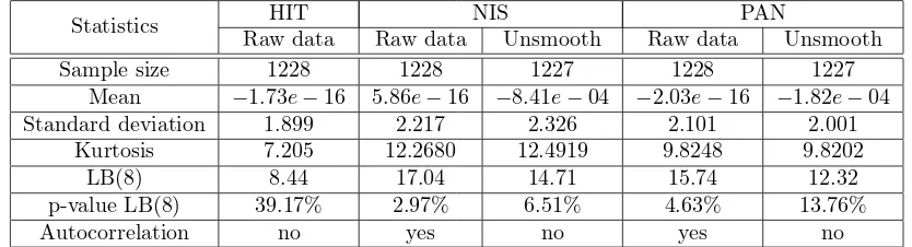
Table 1: Descriptive statistics of daily returns for three stocks of the TOPIX Core 30.
Statistics HIT NIS PAN
Raw data Raw data Unsmooth Raw data Unsmooth
Sample size 1228 1228 1227 1228 1227
Mean −1.73e−16 5.86e−16 −8.41e−04 −2.03e−16 −1.82e−04 Standard deviation 1.899 2.217 2.326 2.101 2.001
Kurtosis 7.205 12.2680 12.4919 9.8248 9.8202 LB(8) 8.44 17.04 14.71 15.74 12.32 p-value LB(8) 39.17% 2.97% 6.51% 4.63% 13.76%
Autocorrelation no yes no yes no
NOTE: The lag lengths= 8 for the LB(s) statistic is selected based on the choice of
s≈ln(1228) (see Tsay (2010)).
3.2 Empirical Results
The hyperparameters required in the joint posterior are set todα = 0,Dα = 10,A= 30,
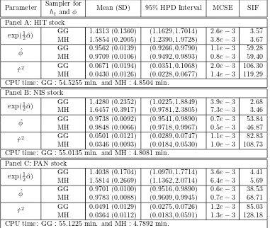
B = 1.5,a= 5 andb= 0.2. The burn-in period of the MCMC simulation consists of 5,000 iterations, and the posterior sample of the parameter consists of N = 10,000 iterations. The MCMC sampler is initialized by setting all the ht = 1, α = 1, φ= 0.9 and τ2 = 0.1. Table 2 summarizes the comparison of the MCMC output, including the posterior mean, the standard deviation (SD) in brackets, the 95% credible interval, the Monte Carlo standard error (MCSE) and the simulation inefficiency factors (SIF). The 95% credible intervals are calculated using a highest posterior density (HPD) proposed by Chen and Shao (1999). The MCSE is useful to check the mixing performance of the MCMC simulation and estimated by bσf/
√
N (see Roberts (1996)), where σb2
f defined as the variance of the posterior mean from correlated draws. Here, the batch size for computing MCSE is 200 and there are 50 batches. The SIF can be interpreted as the number of successive iterations needed to obtain near independent samples and is calculated bybσ2
f/σe2f, whereeσf is the standard deviation of the posterior mean. It is useful to check the efficiency of the algorithm. In addition, we also report the CPU time on a Core2 Duo 2.8GHz with MATLAB version 7.8.0.347(R2009a).
conditional variance of volatility, ˆτ2, are smaller in the MH sampler than those in the GG sampler, indicating that the volatility of the MH sampler is less variable than those of the GG sampler. In computational time, we can see that the GG sampler is relatively greedy because the main cost of the sampler is of course the evaluation of the posterior at each of the grid nodes.
Table 2: Posterior samples of daily returns for three stocks of the TOPIX Core 30.
Parameter Sampler for Mean (SD) 95% HPD Interval MCSE SIF
htandφ
Next, we compare the performance of volatility estimates. To evaluate the estimated volatility accuracy, the realized volatility (RV) is used as a proxy and six loss functions are used (but the statistic values are not reported to save space), namely, root mean-squared error (RMSE) for volatility and variance, mean absolute error (MAE) for volatility and variance, logarithmic loss (LL) and Gaussian quasi-maximum likelihood function (GMLE), as discussed by Bollerslev et al. (1994) and Lopez (2001). The percentage RV is defined
by RVt= 100×
rX
Nt
k=2[p(t, k)−p(t, k−1)]
2, whereN
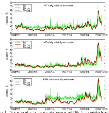
Figure 1: Time series plots for the posterior mean of volatility ˆσt = exp(1
2ˆht) based on the
use of GG and MH samplers for sampling htand φ in the standard LNSV model,
together with realized volatility.
Table 3: Summary of correlation and normality test statistics of standardized innovations.
Statistics GG HIT MH GG NIS MH GG PANMH
LB(8) 7.45 7.59 8.45 8.03 6.24 6.92 p-value LB(8) 48.86% 47.44% 39.08% 43.09% 62.09% 54.52%
JB 5.61 1.63 5.74 2.24 4.84 2.61 p-value JB 6.05% 44.33% 5.68% 32.58% 8.88% 27.18%
3.3 Model Diagnostic
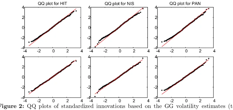
To examine to what the proposed standard LNSV model provides an accurate description of the return dynamics, we consider a measure of goodness of fit based on the standardized innovationsǫt=Rtexp
−12ˆht
stocks and samplers have no significant serial correlation and follow a normal distribution, indicating a quite satisfying return dynamics performance. Figure 2 depicts the QQ plots of standardized innovations. It is shown that the standard LNSV model estimated by MH sampler is more able to capture extreme observations in the tails of the distribution.
Figure 2: QQ plots of standardized innovations based on the GG volatility estimates (top panel) and the MH volatility estimates (bottom panel).
4
Conclusions
This article compares performances between the use of the Griddy Gibbs and Metropolis-Hastings samplers to estimate parameters and latent stochastic processes in the standard log-normal stochastic volatility (LNSV). The results, based on daily observations from three stocks of the TOPIX Core 30: Hitachi Ltd., Nissan Motor Co. Ltd. and Panasonic Corp., reveal that volatility in MH sampler is more persistent and less variable than those in GG sampler. From the use of six loss functions, where daily RV is used as a proxy, it is noted that the GMLE criterion indicates that the GG sampler provides the most accurate volatility, while the results for the other functions indicate no clear pattern. In computational time, the GG sampler is much more costly, although it seems easier to implement, because the main cost of this sampler is on the evaluation of the posterior at each of the grid nodes. Finally, our empirical study indicates that MH sampler is more able to capture extreme observations in the tails of the distribution.
References
Bauwens, L., & Lubrano, M. (1998). Bayesian inference on GARCH models using the Gibbs sampler. The Econometrics Journal,1(1), 23–46.
Bollerslev, T., Engle, R. F., & Nelson, D. B. (1994). ARCH Models. In R. Engle & D. McFadden (Eds.), The Handbook of Econometrics (pp. 2959–3038). Amsterdam: North-Holland.
Carnero, M. A., Pea, D., & Ruiz, E. (2001). Is stochastic volatility more flexible than GARCH? Working Paper 01-08, Universidad Carlos III de Madrid. Retrieved from
e-archivo.uc3m.es/bitstream/10016/152/1/w
Geltner, D. (1991). Smoothing in appraisal-based returns. Journal of Real Estate Finance and Economics,4(3), 327–345.
Geltner, D. (1993). Estimating market values from appraised values without assuming an efficient market. Journal of Real Estate Research,8(3), 325–346.
Ghysels, E., Harvey, A. C., & Renault, E. (1996). Stochastic volatility. In G. Maddala & C. Rao (Eds.), Handbook of Statistics: Statistical Methods in Finance (pp. 119–191). Amsterdam: Elsevier Science.
Hastings, W. K. (1970). Monte Carlo sampling methods using Markov chains and their applications. Biometrika,57(1), 97–109.
Jacquier, E., Polson, N. G., & Rossi, P. E. (1994). Bayesian analysis of stochastic volatility models. In N. Shephard (Ed.),Stochastic Volatility: Selected Readings (pp. 247–282). Oxford University Press, New York.
Kim, S., Shephard, N., & Chib, S. (1998). Stochastic volatility: likelihood inference and comparison with ARCH models. In N. Shephard (Ed.),Stochastic Volatility: Selected Readings (pp. 283–322). Oxford University Press, New York.
Lopez, J. A. (2001). Evaluation of predictive accuracy of volatility models. Journal of Forecasting,20(1), 87–109.
Metropolis, N., Rosenbluth, A. W., Marshall, N. R., Teller, A. H., & Teller, E. (1953). Equations of state calculations by fast computing machines. Journal of Chemical Physics,21(6), 1087–1091.
Metropolis, N., & Ulam, S. (1949). The Monte Carlo method. Journal of the American Statistical Association,44(247), 335–341.
Rachev, S. T., Hsu, J. S. J., Bagasheva, B. S., & Fabozzi, F. J. (2008). Bayesian methods in finance. John Wiley & Sons.
Ripley, B. D. (1987). Stochastic simulation. John Wiley & Sons.
Ritter, C., & Tanner, M. A. (1953). Facilitating the Gibbs sampler: The Gibbs stopper and the Griddy-Gibbs sampler. Journal of the American Statistical Association,87(419), 861–868.
Roberts, G. O. (1996). Markov chain concepts related to sampling algorithms. In R. S. Gilks W.R. & D. Spiegelhalter (Eds.),Markov Chain Monte Carlo in Practice (pp. 45–57). Chapman & Hall, London.
Shephard, N. (1993). Fitting non-linear time series models, with applications to stochastic variance models. Journal of Applied Econometrics,8, 135–152.
Taylor, S. J. (1982). Financial returns modelled by the product of two stochastic processes— a study of the daily sugar prices 1961–75. In N. Shephard (Ed.),Stochastic Volatility: Selected Readings (pp. 60–82). Oxford University Press, New York.
Tierney, L. (1994). Markov chain for exploring posterior distributions. Annals of Statistics,
22(4), 1701–1762.
Tsay, R. S. (2010). Analysis of financial time series. John Wiley & Sons.