Diagrammatic approach to calculation of the fluctuation
correlation matrix in a metabolic system
I. Rojdestvenski
a,*, M.G. Cottam
baDepartment of Plant Physiology,Umea Uni6ersity,Umea90187,Sweden
bDepartment of Physics and Astronomy,Uni6ersity of Western Ontario,London,Ont.,Canada N6A3K7
Received 3 June 1999; received in revised form 21 January 2000; accepted 10 February 2000
Abstract
We present here a simple diagrammatic approach for the time evolution of the fluctuations in metabolite concentrations around the steady state. A fluctuation correlation matrix is introduced to characterise the response in the concentrations of metabolites to a singular initial fluctuation in one of the metabolites. We show how the temporal evolution of the correlation matrix can be represented in the form of a series with individual terms corresponding to pathways on a metabolic graph. The basic properties of such graphs are studied and it is shown how each term in the series can be evaluated. A Monte-Carlo procedure is outlined to calculate the fluctuation correlation matrix. We discuss various properties of the graphical representation and discuss links to information theory that arise from it. © 2000 Elsevier Science Ireland Ltd. All rights reserved.
Keywords:Fluctuation correlation matrix; Metabolite; Monte-Carlo procedure
www.elsevier.com/locate/biosystems
1. Introduction
Recently considerable attention has been paid to theoretical studies in the field of metabolic control and regulation. Since the seminal work by Kacser (see Kacser and Burns, 1973), where a metabolic control analysis via control coefficients was introduced, many papers have been devoted to developing both theoretical and experimental
methods for calculating and measuring the
metabolic control coefficients. In particular, con-siderable effort has been put into studying the properties of the matrix of control coefficients (e.g. Cascante et al., 1996; Giesrch, 1997; Elsner and Giersch, 1998), the ways to introduce time-scale hierarchies (Delgado and Liao, 1995), spatial blocking (Brand, 1996; Rohwer et al., 1996; Ain-scow and Brand, 1998), and ‘asynchronous
au-tomata’ metaphorae of regulatory networks
(Thomas, 1991).
While many of these works used graphical rep-resentations for the metabolic pathways, the es-sential part of the analysis was done mainly by applying matrix algebra. The graphs of metabolic pathways played only an illustrative or qualitative
* Corresponding author. Tel.:+46-70-7195291; fax:+ 46-90-7866676.
E-mail address: [email protected] (I. Rojdestvenski)
role. By contrast, in statistical physics and quan-tum field theory, graphical representations have for a long time been viewed in a much wider context than just as illustrations. A well-known example is a formalism of Feyninan diagrams (see Ryder, 1985) in quantum field theory. The pur-pose of the present paper is to discuss a possible method of introducing a quantitative diagram-matic technique in the analysis of metabolic net-works. This will enable us to put the term ‘metabolic pathway’ in a more rigorous algebraic context. We should mention here that a more rigorous approach along basically the same math-ematical scheme is presented in (Rojdestvenski and Cottam, 2000).
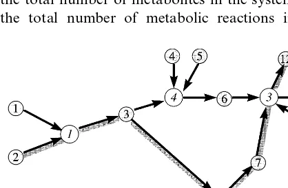
A metabolism can be described completely if one knows how the concentrations of all the metabolites in the system vary with time. It is convenient to describe a metabolism schematically by means of an ordered directed graph, such as the example given in Fig. 1. The vertices that are depicted by shaded circles denote ‘pools’ of metabolites; they are each labelled by an integeri where i[1, 2, ..., N]. The vertices that are de-picted as open circles denote metabolic reactions; likewise they are each labelled by an integerm[1, 2, ..., M]. Here Nand M stand, respectively, for the total number of metabolites in the system and the total number of metabolic reactions in the
system. The arrow directed from a ‘poor’ vertex i to a ‘reaction’ vertex m indicates that i is a sub-strate for m, while the arrow from a ‘reaction’ vertex m to a ‘pool’ vertex i indicates that i is a product of m. This representation deviates slightly from the conventional one, with the vertices here being employed not only for metabolites but for reactions as well. This is done for later algebraic convenience, but it also bears some meaning apart from that. Indeed, in many diagrammatic tech-niques the arrow represents a relation, or a func-tion, while vertices stand for the material entities connected by this relation. A reaction sets up a correspondence between products and substrates. In this sense reaction represents a function (in mathematical sense),
{reaction substrates}reactionl {reaction products} On the other hand, reaction is at the same time a function and a material entity (represented by the enzyme). This is a common situation when studying biological systems, which are essentially autopoietic, i.e. represent systems in which certain relations between their elements are included in these systems as new elements. We may argue here that, philosophically speaking, in biological systems the difference between the thing and its representation, formulated by Kirby (1998), often vanishes. Kirby writes, ‘‘Representations denote classes; things are individual. Representations cannot themselves evolve like (certain) things; they can only be changed. A representation does not go out in the world and function; the thing it represents, or for whom it meditates, does’’. The point is that the representation in Kirby’s notion does not become part of the described (repre-sented) system. On the other hand, the above duality of a reaction, representing a functional relation between material objects (metabolites), is, in turn, represented by another material entity (enzyme). Going further up the description hier-archy, enzyme description is encoded in the genome. Genome thus becomes a description (representation) of material objects (enzymes), at the same time being itself represented by material entities (DNA, RNA). Moreover, often, as in the case of certain autocatalytic reactions, as well as for those enzymes which catalyse gene expression
processes, the differences between the ‘things’ and their ‘representations’ become even more blurred. Such a situation is described (Nalimov, 1981) as mixing metalanguage into language. The above paradoxical ‘language game of living matter’ is, however, too involved for a brief discussion here. In our scheme this ‘material’ aspect of the reaction (function) is emphasised, with the arrows describing relations between metabolites and reac-tions (i.e. the properties of being either a substrate or a product). Very often metabolism is also described in terms of ‘pathways’. A common-sense definition of a pathway is quite obvious, namely it is a sequence of reactions sharing a common mass flow. An example of such a path-way is given by the thick line running through Fig. 1.
The time evolution for the metabolic concentra-tions can be conveniently expressed in terms of a ‘time-evolution’ operator. This operator acts on the concentration vector for the initial conditions (i.e. the vector comprising the values of the con-centrations at time t=0) to produce the
concen-tration vectors at a later time t. Our goal in
developing the theory is to write the time-evolu-tion operator for the system of metabolic equa-tions as a superposition of operators representing the propagation along all the possible pathways of the given metabolic system. Then the weights of the pathways would be functions of time, rep-resenting the relative ‘importance’ of the path-ways at a given moment of time. We shall develop this into a systematic diagrammatic procedure for evaluating the variations (in time) of the metabo-lite concentrations.
2. Analysis of the fluctuations about the steady state
We start with the rate equation written in the following general form:
dx
dt=v(x) (1)
where x denotes the vector of concentrations,
whilev(x)={6
i({xj})} stands for the vector
com-prising the rates of change of the concentrations. In general, these latter quantities depend on the concentrations of metabolites in the system. In the steady state situation, corresponding tox=x0, we
have by definition
dx0
dt =0 (2)
and hence v(x0)=0.
Typically, a system of coupled equations can be efficiently characterised by the time evolutions of small fluctuations around the steady state. Such an approach, for example, forms the basis for the theory of fluctuations in statistical physics (e.g. Landau and Lifschits, 1979), as well as the metabolic control analysis (MCA) method in bio-chemistry (e.g. Kacser and Burns, 1973). The analysis of the time evolution of fluctuations, and the correlations between them, can help in deter-mining the stability of the steady (or equilibrium) state against changes in the external conditions. Indeed, provided the steady state x0is stable, the
fluctuations in concentration (which may initially be present in the system at t=0) would tend to
vanish in the limit of t . By contrast, an
unstable steady state would yield growth of the initially small fluctuations.
Here we discuss the behaviour of small fluctua-tions in the concentrafluctua-tions around the steady state of a metabolic system. For this purpose we represent the state of the system as
x(t)=x0 +n(t)
v(x):v(x0)+D·n (3)
where the operator D can be regarded as a
con-stant (in time) N×Nmatrix with the elements
Dij=(6i (xj
)
x=x0
(4)
Also n is an N-dimensional fluctuation vector
defined by
n=
Æ Ã Ã Ã È
n1
n2
… nN
Ç Ã Ã Ã É
=% N
i=1
with the vector ei forms an orthonormal basis in
the N-dimensional space of concentrations.We
also have the property e1e2 … eN=IN
(theN×Nidentity matrix). The equation of mo-tion for n then reads:
dn
dt=D·n (6)
which yields a formal (operator) solution
n(t)=eDt·
n(0) (7)
for the time evolution of the fluctuations. It is useful also to introduce a correlation matrixCas the matrix whose elements are
Cij=eieDtej (8)
This quantity characterises the correlations be-tween the fluctuations of concentrations of the different metabolites. Specifically Eq. (8) charac-terises what would be the contribution to the concentration of theith metabolite at timet
pro-duced by a singular perturbation of the jth
metabolite at zero time. The (appropriately defined) correlation function takes account of the interactions present in the system, and it yields the
characteristic times associated with these
interactions.
We proceed next to the pathway representation as a means to carry out the evaluation of the above quantities. Eq. (7) may first be expanded as a power series with respect to time as
n(t)= %
We may then decompose the vector v and the
matrixDinto sums of terms corresponding to the different elementary metabolic reactions, giving
6i= % M
m=1
hmi6m (10)
Here 6m denotes the rate of the mth reaction and
hmi is the stoichiometric coefficient of metabolite i
in this reaction. Also, we may write
D= %
m is the elasticity of the enzyme
m with respect to the metabolite j (see Cornish-Bowden, 1995). As before, M denotes the total number of metabolic reactions in the system. Expanding the exponential in Eq. (9) in Taylor series and using Eq. (11) we rewrite Eq. (9), by analogy to the Handscomb representation (Handscomb, 1962; Rojdestvenski and Cottam, 2000), in the form
n(t)= %
different reactions. What we call here, for histori-cal reasons, the ‘Handscomb representation’ is, in fact, a series expansion that forms the foundation of any diagrammatic technique in statistical me-chanics (see Rivers, 1987).
The operator products in Eq. (12) represent the contributions from different reaction sequences. The expansion may now be used to rewrite Eq. (8) as
In terms of the matrix elements this result becomes
In order to proceed further we now make some assumptions about the reaction rates in Eq. (1) and the corresponding matrix elements appearing in Eq. (14). We should note that these, or similar, assumptions are typical of previous MCA theories (see Cornish-Bowden, 1995).
1. We assume that the reaction rate for any reactionmmdoes not depend on the
concentra-tion of those metabolites that do not partici-pate in this reaction. Thus a necessary condition for any term in the expansion (Eq. (14)) to be nonzero is:
Öm, km, km−1mm, (15)
which means thatkmandkm−1are each either
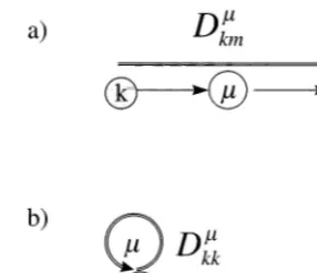
Fig. 2. A graphical representation of the terms contained in Eq. (18), (a) aDkmm matrix element withk"m(an arrow); (b)
a ‘diagonal’Dkmm matrix element (a loop).
sation. This, however, will not be considered in this introductory account.
Using Eqs. (15) – (17) we now may rearrange the terms in Eq. (14) to give
Cij= %
r=0
tr
r!%Gr
Dij(Gr)(−1) nss(Gr)+npp(Gr)+nloop(Gr) 5
r
m=1 Dkmjm
mm , (18)
where it is now the absolute values of the D
coefficients that appear. These terms can be repre-sented diagrammatically as shown in Fig. 2. In Eq. (18) we introduce new objects, ordered index sets,Gr={i1, …,ir} in which each indexim
corre-sponds to a ‘path’ from a ‘pool’ vertex kim
through a ‘reaction’ vertex mim to another ‘pool’
vertex, jim, with a connectivity requirement that
ÖGr, Öm, kim=jim−1 (19)
Also the function Dij(Gr)=1 ifGr, starts from
the pool vertex i and ends at the pool vertex j otherwise Dij(Gr)=0. The other new notations
and terminology are explained below.
GraphicallyGr, can be represented as a ‘route’,
or a pathway, on the metabolic graph. EachGr, is
a connected ordered graph, i.e. it can be drawn without lifting a pen from the paper, which is a direct consequence of Eq. (19). It contains its own sequence of arrows, corresponding to the direc-tion, say, from a pool vertexkto pool vertexj(so
that a distinction is made between
Dkj m
and Djk m
), as well as ‘single index loops’ for the terms of the type Djjm. From now on we will
use the term M-arrows for the arrows on a
metabolic graph proper, that correspond to the substrate – product relations, and we will name G-arrows the arrows that specify the direction in a Gr, graph. An example of a Gr, graph (with
r=4) for part of the metabolic graph in Fig. 1 is presented in Fig. 3, its contribution being
Fig. 3. A sample G-graph comprising a part of the metabolic graph in Fig. 1. The M-arrows are represented by solid fines.
2. We assume that any reaction rate is inhibited by an accumulation of product(s) and en-hanced by an accumulation of substrates (see also a study on signs of control coefficients by Sen (1996)). This implies the following sign rules:
hmk (6m(x k
x=x0
B0. (17)
It should be noted that, although the above assumptions are required for the version of dia-grammatic technique to be formulated here, some of the conditions allow straightforward
hmk(6m
(x j
x=x0
à à Ã
\0, if k is a substrate of m and j is a product, or vice versa
−t
numbers of G-arrows in Gr, which connect,
re-spectively, substrate to substrate (e.g. the G-ar-rows 34 and 45 in Fig. 3) and product to product, while nloop stands for the number of
looped G-arrows in Gr, (e.g. single index loop
33 in Fig. 3). The overall negative signs in Eq. (18) that are associated with each loop, substrate – substrate and product – product G-arrows are con-sequences of Eq. (16).
Now we can formulate the rules for calculating the individual terms of Eq. (18) on any complete metabolism graph. The recipe is as follows:
1. Draw the complete metabolic scheme, with the reactions and pools depicted by vertices, as explained above (i.e. like in Fig. 1).
2. Define an entry point i at a corresponding
‘pool’ vertex, and an exit point at jth ‘pool’ vertex.
3. Draw all possible pathways Gr, that start at i
and end at j, allowing for possible repetitions (i.e. a bouncing back and forth between the reaction and pool vertices and loops around pool vertices).
4. For each pathway count the nss, nppand nloop
quantities.
5. Finally, write the contribution for a given pathway as:
3. Monte-Carlo evaluation of the relative contributions of different metabolic pathways
We now rewrite the preceding formalism in a way that will be suitable for applying Monte-Carlo numerical simulations. First Eq. (20) can be re-expressed in terms of a ratio of two mean values:
These justify our usage of the functions p(Gr)
as probability distribution in Eq. (22), where the angular brackets denote an average value taken with respect to the distribution p(Gr).
A general Monte-Carlo procedure to calculate the ratio in Eq. (22) may now be implemented as follows:
1. We set up a Markov chain in the space of all possible pathways Gr with a limit distribution
given by p(Gr).
2. At each step we generate a certain pathwayGr.
3. We calculate its overall sign contribution j(Gr).
6. After a predefined (and substantial) number of steps we calculate Eq. (22) as:
Cij
As regards methods for a practical implementa-tion of the Markov chain, the most obvious can-didates may be either some sort of ‘percolation’ procedure (see Hinrichsen and Koduvely, 1998) or a Handscomb-type procedure (Handscomb, 1962; Rojdestvenski and Cottam, 2000). The latter
im-plies sampling the space of all Gr graphs via
by adding an arrow, or decreaser by eliminating one of the arrows, namely
GrGr(Dkr+1jr+1
mr+1 ) Gr=G
r−1(Dkrjr
mr )G
r−1
Unfortunately, these straightforward
ap-proaches are impractical in many cases. The rea-son is the well known ‘sign problem’, which is frequently encountered in theoretical physics ap-plications that deal with diagrammatic expansions (see Rozhdestvensky and Favorsky, 1992). In-deed, the numerator and denominator in Eq. (23) may be infinite sums comprising terms with alter-ing signs. Different signs arise here because of the rules (Eqs. (16) and (17)). The numerical values of such sums are typically determined with consider-able uncertainty and their ratios may be com-pletely ill defined. Such a situation in the quantum Monte-Carlo simulations of antiferromagnetic systems is described, for example, by Rojdestven-ski (1995). Some possible ways to deal with this problem are either to concentrate on specific cases where this sign problem does not appear (as in Handscomb, 1964) or to choose a different repre-sentation of variables (as in Rozhdestvensky and Favorsky, 1992). We will discuss, in fact, a combi-nation of these two approaches in application to the current problem.
4. Two types of branching in metabolic graphs
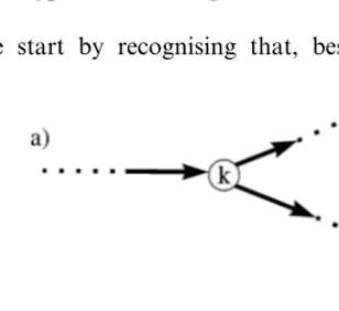
We start by recognising that, besides the
in-evitable loops, the negative signs in Eq. (18) ap-pear whenever the chosen metabolic system contains reactions that have more than one sub-strate (product). An example of such situation might be branching points (basically, all the reac-tion vertices appearing in Fig. 1). Suppose we now restrict our attention to metabolic systems consist-ing of reactions that have just one substrate and
one product. For such reactions all Gr have
nss(Gr)=npp(Gr)=0.
We should note that this does not rule out branching completely. In fact, there are two possi-ble types of branching in metabolic systems. One may be called ‘metabolite’ branching, where one metabolite is a substrate (or a product) of two reactions in different branches. Several examples of such branching may be found, for instance, in the dark reactions of photosynthesis, such as transformation of glucose-6-phosphate via two pathways — glycogen biosynthetic pathway, with 6-phosphate being converted into glucose-1-phosphate by action of phosphoglucornutase enzyme, and penthose phosphate pathway in which the same glucose-6-phosphate is converted into 6-phosphogluconolactone by action of G6P dehydrogenase. Diagrammatically this type of sit-uation is shown in Fig. 4a.
Another branching type, termed ‘enzyme’
branching, takes place if a certain reaction itself is a branching point. Specifically, it produces two or more products further used in different metabolic branches (and/or utilises two or more substrates coming from different metabolic branches), as shown in Fig. 4b. Example of such type of branching can also be found in the penthose phosphate pathway, with glyceraldehyde-3-phos-phate and sedoheptulose-7-phosglyceraldehyde-3-phos-phate both being substrates for the reaction catalysed by transaldo-lase enzyme, which results in two products being erythrose-4-phosphate and fructose-6-phosphate.
Although it substantially narrows the appli-cability of the procedures, the above restriction allows tackling a few practically interesting situa-tions. These include the simplest case of linear metabolic chain (Fig. 5a), a linear chain coupled to a ‘futile’ cycle (Fig. 5b), and two linear chains coupled by a cycle (Fig. 5c).
Fig. 5. (a) A simple linear metabolic chain; (b) a linear metabolic chain coupled to a futile cycle; (c) two simple metabolic chains coupled via a two-enzyme cycle.
Cij=e−lt %
r=0
tr
r!%Gr
Dij(Gr)5 r
m=1 D0 kmjm
mm (30)
where all the terms in the summation are positive. Consequently, Eq. (23) simplifies to
Cij
% k,l
Ckl
=Dij(Gr)p(Gr) (31)
This can now be calculated by means of slightly modified Handscomb method (see Handscomb, 1962; Rojdestvenski and Cottam, 2000), asAand Bin Eq. (26) become, respectively, the number of Markov chain steps resulting in graphs starting at i and ending at j, and the total number of steps. As always, the ultimate practicality of such an approach can only be tested by attempting calcu-lations for real systems and comparing the Monte-Carlo simulation data with results ob-tained using other methods, which we plan to do in near future.
6. Discussion and conclusions: metabolic graphs and information theory
Information theory and its applications (in par-ticular, via the Shannon – McMillan theorem) to biology have been discussed for a number of years. Several trends prevail in this discussion as we have outlined in detail in Rojdestvenski and Cottam (2000). We will remind here some of our arguments.
One trend views a biological system as a com-puting device: a computer in its own right (Liber-man and Minina, 1995; Fernandez and Belinky, 1996; Benera and Nanjundiah, 1997; Rambidi, 1997; Schmitt and Herzel, 1997; Conrad and Za-uner, 1998) or as a linguistic information process-ing in device (Ji, 1997). The examination of biological information processing in terms of a universal Turing machine is given by Kampis (1996).
Another trend seeks to form a link between information theory and biology via the physical description of biological systems and via the con-cept of entropy, which is common to statistical
5. Elimination of the negative signs
Apart from the restrictions discussed above, we still face the problem of negative signs arising from the contributions from loops. We may, how-ever, eliminate all the negative contributions using a mathematical transform similar to that em-ployed by Rozhdestvensky and Favorsky (1992).
First we notice that the loops represent diago-nal elements of the D matrix and that Dkkm B0.
Also we may rewrite Eq. (8) in the form:
Cij=eie
-lIteD0tej=e−lt[e ie
D0te
j], (28)
where we define (for any constantl)
D0ij=Dij for i"j and D0ii=Dii+l. (29)
Now we may choose l to be sufficiently large and positive thatÖi, D0 ii\0. With this result, and
physics and information theory (Gudkov, 1978; Torres, 1990; Waltz, 1992).
There are, however, other possibilities. As it is quite often, the case in many branches of science where mathematics is used as a tool, a new repre-sentation of an old problem brings fresh allusions to other problems via similarities in the mathe-matical formalisms. The following is a description of how the graphical representation (see Eq. (18)) provides a link between metabolism theory and information theory.
Suppose we have a source of information, X,
which produces sequences of ‘signals’ of lengthn, each signal being taken from a certain alphabet. We now define, following Wallace and Wallace (1998), the source uncertainty as follows:
H[X]=lim
n
log[N(n)]
n (32)
whereX is the source and N(n) is the number of ‘meaningful’ sequences of length n produced by the source. It is important to stress a strong context dependence of Eq. (32), namely, what is a ‘meaningful sequence’. Ash (1990), as cited in Wallace and Wallace (1998), points out that a ‘‘large uncertainty means… a large number of ‘meaningful’ sequences (of a given lengthn). Thus given two languages with uncertaintiesH1andH2,
respectively, if H1\H2, then in the absence of
noise it is easier to communicate in the first language, more can be said in the same amount of time (i.e. for a givenn). On the other hand, it will be easier to reconstruct a scrambled portion of text (caused by noise in the communication chan-nel) in the second language, since fewer of the possible sequences of lengthn are meaningful’’.
The sequences of signals in Eq. (32) are merely n element long ordered sets that are produced by a certain processX, and each element of them is taken from a certain ‘alphabet’. Hence, if one finds a representation of a problem in, say, physics or biology that presents the solution in the form of such sequences, then the mapping of this problem to information theory is achieved. In fact, many statistical physics problems deal with series expansions with respect to certain multiple indices, and this makes them good candidates for seeking such a mapping.
Finally let us discuss a possible mapping of the ‘pathway’ representation (Eq. (18)) to information theory, similar to Rojdestvenski and Cottam (2000). We may take the space of Gr, sets as a
space of signal sequences. Indeed, letXin Eq. (32) be a random triple index variable taking the val-ues denoted by (i,j,m), 15m5M, 15i, j5N. Then, all the Gr, sets can be mapped to all the
possible signal sequences, generated by the source X. Let us call a set of all possible values of the triple index an ‘alphabet’. Then we may refer to Gr, as being an r-letter ‘sentence’.
To develop our mapping further we note that for the definition in Eq. (32) one must determine what ‘meaningful’ sequence means in our context. This notion strongly depends on the situation (i.e. on the ‘alphabet’). However, once this has been rigorously established, the use of Eq. (32) is straightforward. In our case let us assume that ‘sentence’ Gr, is meaningful once its probability
p(Gr), as defined in Eq. (23), is nonzero.
More-over, let us also quantitatively describe ‘meaning’ by the numerical value of the probability p(Gr).
On the other hand, each Gr, implies a chain of
certain reaction operators put in certain order, or, in other words, represents a certain sequence of reactions, which can loosely be called a ‘pathway’. The numerical coefficient associated with a path-way in Eq. (18) or Eq. (23) may be called the ‘meaning’ of that pathway. In the course of Monte-Carlo simulation for different times t in Eq. (23) the system will relax into different ‘typi-cal’ subsets GrVr(t), with a certain ‘typical’ r
associated with it. The Gr from such subsets will
reliable experimental results (easy error correc-tion).
Pathway representation also brings about an-other aspect of information theory. As a matter of fact, switching from concentration representation to pathway representation means changing lan-guage of description. The question of optimal language of description is closely linked with the concept of complexity. Indeed, the Kolmogorov definition of complexity of a system states, in plain language, that it is the shortest possible description of this system, made in a language understandable by the universal Turing machine. Reference to the universal Turing machine is present simply because the complexity of a system consists of two compo-nents. These components are the length of descrip-tion in a chosen language of descripdescrip-tion, and the length of description of this language (alphabet) itself in terms of the Turing machine language. Minimisation of description for the sake of obtain-ing complexity is an interplay between these two components. Indeed, the description of a system (or a class of systems) in a certain language may be very short, but the language itself may be very rich, and require long description.
Let us discuss, although briefly and sketchy, the pathway representation within this ‘language’ framework. We call ‘equilibrium subspace’ a set of such sequences, which (in a given context) have appreciable meaning (i.e. probability). The source is always limited to this subspace, as other se-quences have vanishing probabilities. In fact, in a given context, which means given probability dis-tribution that depends on time (Eq. (23)) and on other factors changing matrix elements ofD, it is only the equilibrium subspace that matters. Those sequences that have vanishing or zero probabilities in expansion (Eq. (22)) for a given context simply do not exist in this context. We may show how in this case a new language of description can emerge by way of analysing the sequences from the equi-librium subspace as sequences of ‘letters’ from an alphabet. In equilibrium subspace we may attempt, by way of calculating the Kolmogorov complexity of the sentence, to modify the language in the following way:
Suppose we have an alphabet, a1, …, aN. The
description of a sentence of length L would
comprise Npositions occupied by the descrip-tion (listing) of the alphabet, and L positions specifying the order of ‘letters’ in the sentence. The length of the description would then be
C=L+N.
Suppose the equilibrium subspace appears to
comprise sentences which are very likely to have a certain short subsequence ‘ail, …,aik’ in
them, maybe repeated several times. Then we may add a letter to our alphabet,b, that would ‘nominate’ this subsequence, b=‘ail, …, aik’.
Then, if our chosen sequence contains the sub-sequenceb Mtimes,M\k, then the length of description will be C%=(L+N)−M×(k−
l)+k. Here the second term comes from the
fact that we replace ksymbols of the sequence b by one symbol, b. The third term originates due to the necessity to describe b in terms of ‘base’ language {a1, …, aN}. In view of a
proper definition of complexity, that is a mini-mal description, we have to use C% instead of
C. Hence we have a strong contextual depen-dence of the complexity, and the alphabet. This is precisely the ‘language game’ of Witgenstein, and the emerging ‘additions’ to the alphabet which, for the sake of description minimisa-tion, must be longer than one symbol (see above), manifest emerging structures.
As different contexts provide different equi-librium subspaces, the C% descriptions and
corre-sponding languages of description differ from one context to another. Coming back to pathway representation we may note that the weights of different pathways in different conditions vary for any definition of a pathway, be it an intuitive definition of a chain of reactions or our graph based scheme. In some conditions, for instance, it may so happen that all the metabolic graphs would resort to a single pathway, with all other possible pathways having vanishing probabilities. In this case pathway representation would have an advantage compared with representing the sys-tem by metabolic concentration vector, or reac-tion rates vector, as the descripreac-tion using the ‘pathway’ alphabet would be more economic.
possibili-ties for utilisation. First, one can take it as a potentially useful formalism to apply in combina-tion with the theory of control coefficients. Second, it brings about a connection with information theory, and this is of particular interest in view of the emerging concept of biological systems as information processing entities. Last, but not the least, it embodies the notion of a pathway, which is defined naturally and quantitatively, and this may lead to a different quantitati6e language for
description of metabolic processes.
Acknowledgements
This work has been supported by Swedish Na-tional Research Council (NFR) and by STINT Agency, Sweden.
References
Ash, R., 1990. Information Theory. Dover, New York. Ainscow, E.K., Brand, M., 1998. Control analysis of systems
with reaction blocks that ‘cross-talk’. Biochim. Biophys. Acta 1366, 284 – 290.
Brand, M., 1996. Top down metabolic control analysis. J. Theor. Biol. 182, 351 – 360.
Benera, N., Nanjundiah, V., 1997. trans Gene regulation in adaptive evolution: a genetic algorithm model. J. Theor. Biol. 188, 153 – 162.
Cascante, M., Puigjaner, L., Kholodenko, B., 1996. Steady-state characterization of systems with moiety-conservations made easy: matrix equations of metabolic control analysis and biochemical system theory. J. Theor. Biol. 178, 1 – 6. Conrad, M., Zauner, K.-P., 1998. DNA as a vehicle for the
self-assembly model of computing. Biosystems 45, 59 – 66. Cornish-Bowden, A., 1995. Fundamentals of Enzyme Kinetics.
Portland Press, London.
Delgado, L., Liao, L.C., 1995. Control of metabolic pathways by time-scale separation. Biosystems 36, 55 – 70.
Elsner, L., Giersch, C., 1998. Metabolic control analysis: separable matrices and interdependence of control coeffi-cients. J. Theor. Biol. 193, 649 – 661.
Fernandez, A., Belinky, A., 1996. Information generation and the loss of conformational entropy during RNA folding. J. Phys. A: Math. Gen. 29, L433 – L438.
Giesrch, C., 1997. Co-response coefficients, monovalent units, and combinatorial rules: unification of concepts in metabolic control analysis. J. Theor. Biol. 189, 1 – 9.
Gudkov, N.D., 1978. Balance of entropy in photosynthesis. Biofizika 23, 859 – 863 in Russian.
Handscomb, D.C., 1962. The Monte-Carlo method in quantum statistical mechanics. Proc. Cambridge Phil. Soc. 52, 594. Handscomb, D.C., 1964. Monte-Carlo method and the
Heisen-berg ferromagnet. Proc. Cambridge Phil. Soc. 60, 115. Hinrichsen, H., Koduvely, H.M., 1998. Numerical study of local
and global persistence in directed percolation. Eur. Phy. J. B 5, 257 – 264.
Ji, S., 1997. Isomorphism between cell and human languages: molecular, biological, bioinformatic and linguistic implica-tions. Biosystems 44, 17 – 39.
Kacser, H., Burns, L.A., 1973. The control of flux. In: Davies, D.D. (Ed.), Rate Control of Biological Processes. Cam-bridge University Press, CamCam-bridge.
Kampis, G., 1996. Self-modifying systems: a model for the constructive origin of information. Biosystems 38, 119 – 125. Kirby, K.G., 1998. Exaptation and torsion: toward a theory of
natural information processing. Biosystems 46, 81 – 88. Landau, L.D., Lifichits, E.M., 1979. Statistical Physics.
Perga-mon Press, Oxford.
Liberman, E.A., Minina, S.V., 1995. Molecular quantum com-puter of neuron. Biosystems 35, 203 – 207.
Nalimov, V., 1981. In: Colodny, R.G. (Ed.), The Labyrinth of Language: A Mathematician’s Journey. ISI Press, Philadelphia.
Rambidi, N., 1997. Biomolecular computer: roots and promises. Biosystems 44, 1 – 15.
Rivers, R.L., 1987. Path Integral Methods in Quantum Field Theory. Cambridge University Press, Cambridge. Rohwer, J.M., Schuster, S., Westerhoff, H.V., 1996. How to
recognize monofunctional units in a metabolic system? J. Theor. Biol. 179, 213 – 228.
Rojdestvenski, I., 1995. Dynamic and Thermodynamic Proper-ties of the Quasi-Two-Dimensional Magnetic Systems. Ph.D. Thesis, University of Western Ontario, London, Canada.
Rozhdestvensky, I.V., Favorsky, I.A., 1992. Handscomb Monte-Carlo method for S=1/2 transverse ising model. Mol. Simulations 9, 213 – 222.
Roidestvenski, I., Cottam, M., 2000. Mapping of statistical physics to information theory with application to biological systems. J. Theor. Biol. 202, 43 – 54.
Ryder, L.H., 1985. Quantum Field Theory. Cambridge Univer-sity Press, Cambridge.
Schmitt, A.O., Herzel, H., 1997. Estimating of the entropy of DNA sequences. J. Theor. Biol. 188, 369 – 377.
Sen, A.K., 1996. On the sign pattern of metabolic control coefficients. J. Theor. Biol. 182, 269 – 275.
Thomas, R., 1991. Regulatory networks seen as asynchronous automata. J. Theor. Biol. 153, 1 – 23.
Torres, J.-L., 1990. Information, photosynthesis and tempera-ture of the earth. J. Theor. Biol. 144, 131 – 137.
Wallace, R., Wallace, R.G., 1998. Information theory, scaling laws and the thermodynamics of evolution. J. Theor. Biol. 192, 545 – 559.